SLAC–PUB–9047
November 2001

Abstract

In this talk I show how to canonically quantize a massless scalar field in the background of a Schwarzschild black hole in Lemaître coordinates and then present a simplified derivation of Hawking radiation based upon this procedure. The key result of quantization procedure is that the Hamiltonian of the system is explicitly time dependent and so problem is intrinsically non-static. From this it follows that, although a unitary time-development operator exists, it is not useful to talk about vacuum states; rather, one should focus attention on steady state phenomena such as the Hawking radiation. In order to clarify the approximations used to study this problem I begin by discussing the related problem of the massless scalar field theory calculated in the presence of a moving mirror.

Presented at the Workshop on
Light-cone physics: particles and strings, TRENTO 2001
September 3 – September 11, 2001

1 Introduction

The phenomenon of Hawking radiation has fascinated physicists ever since Hawking’s 1974 paper[2] showed that, when quantum fields are taken into account, a black hole of mass $M$ appears to emit (nearly) thermal radiation with a temperature $T_{\rm H}=1/(8\pi GM)$. This result, extensively studied in the literature (see for example [3, 4, 5]), is clearly robust since all approaches lead to the same conclusion. So far as I know, however, no derivation of Hawking radiation discusses the problem within the framework of canonical quantization. This is one reason the question of whether the time evolution of the system is unitary became a topic of debate.

In this talk I present work[1] done in collaboration with Kirill Melnikov, showing that a simple canonical quantization procedure exists and leads to the usual Hawking results within the framework of a unitary quantum theory. This theory has some surprising features but doesn’t seem lead to paradoxes which invalidate the approach. One unique advantage of our calculation is that we can compute the energy-momentum tensor at all positions and times. This allows us to explicitly exhibit transient behavior and retardation effects, and – as a matter of principle – give a self-consistent treatment of back reaction.

Before diving into details I will spend a few moments reminding you why carrying out a Hamiltonian formulation of the problem of a massless scalar field in the presence of a black-hole background seems so difficult. Consider the usual Schwarzschild metric for a black hole of mass $M$:

$$ds^{2}=-(1-{2M\over r})\,dt^{2}+{1\over(1-{2M\over r})}\,dr^{2}+r^{2}d\Omega^{2}$$ (1)

and a massless scalar field with Lagrange density

$${\cal L}=\sqrt{-g}\left[g^{\mu\nu}\,\partial_{\mu}\phi(x)\,\partial_{\nu}\phi(x)\right].$$ (2)

(Note that in what follows I will set $2M=1$ to simplify the equations.) While one usually focuses on the singularity of the metric at $r=2M$, this coordinate singularity is not a problem. The real issue is that in order to canonically quantize this theory we need a family of spacelike slices which foliate the spacetime. Given this, we can then define the field and its conjugate momentum on one of these slices. Inspection of the metric, Eq.1, shows that surfaces of constant Schwarzschild time change from spacelike to timelike at the horizon ($r=2M$) and so, they do not fulfill our requirements.

2 Summary of Results

In order to define a set of spacelike surfaces which foliate the Schwarzschild spacetime we begin by introducing Painlevé coordinatess because surfaces of constant Painlevé time extend from $r=0$ to $r=\infty$ and are everywhere spacelike. Since, however, the Painlevé timelines are not everywhere timelike we will have to make one more transformation, to Lemaître coordinates, in order to canonically quantize the theory. In these coordinates we see that the metric and therefore the Hamiltonian is explicitly time dependent, which is the reason why Hawking radiation exists. Of course, despite the time dependence of the Hamiltonian, the theory possesses a unitary time development operator, which is all we need to discuss the relevant physical issues. Note, because the Hamiltonian is time dependent, it is never useful to talk about eigenstates.

The strategy of the computations I will describe goes as follows: first, we canonically quantize the theory; second, we devise a scheme (the Geometric Optics Approximation) for approximately solving the Heisenberg equations of motion (this is easier than calculating the unitary time development operator); third, we compute the temperature seen by a thermometer located at fixed $r$ which is adiabatically switched on and off; last, we compute the flux passing through a sphere of fixed radius and show that in the long time limit (after transients have died out) it has the Hawking value.

3 Review of Coordinate Systems

While we are ultimately interested in the surfaces defined by fixing Painlevé time, it is convenient to first introduce Kruskal coordinates and plot the various surfaces of interest in these coordinates. The reason for this is that these coordinates make it particularly easy to draw null-geodesics (they are simply lines parallel to either the $X$ or $Y$ axes shown in Fig.1) and they allow us to easily compare surfaces of fixed Schwarzschild time to surfaces of fixed Painlevé time. Kruskal coordinates are defined by the equations:

$$xy=(r-1)\,e^{r}\qquad,\qquad{x\over|y|}=e^{t_{S}}.$$ (3)

In these coordinates the Schwarzschild metric becomes:

$$ds^{2}={32\,e^{|-r|}dx\,dy\over r}+r^{2}d\Omega^{2}$$ (4)

Note that Eq.3 immediately shows us that fixed Schwarzschild $r$ is a hyperbola in the $x,y$-plane, as shown in Fig.1, and that surfaces of fixed Schwarzschild time corresponds to straight lines $x=|y|\,e^{t_{S}}$ (which are not shown in Fig.1).

Now, Painlevé coordinates are arrived at by making an $r$-dependent shift in Schwarzschild time; i.e.,

$$t=\lambda-2\sqrt{r}-\ln\left(\left|{\sqrt{r}-1\over\sqrt{r}+1}\right|\right)$$ (5)

These are the almost horizontal curves shown in Fig.1 which clearly foliate the spacetime. Note, that while Schwarzschild $t$ and Painlevé $\lambda$ differ by functions of $r$, if two events having the same $r$ then the differences in Schwarzschild and Painlevé times are equal. In Painlevé coordinates the Schwarzschild metric takes the form

$$ds^{2}=-(1-{1\over r})\,d\lambda^{2}+{2\,d\lambda\,dr\over\sqrt{r}}+dr^{2}+r^{2}d\Omega^{2}$$ (6)

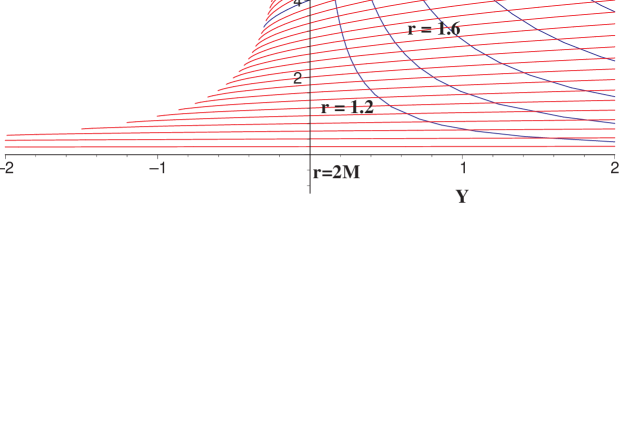
Figure 1:

Although Painlevé coordinates are useful for defining our set of spacelike surfaces they don’t work well for canonical quantization because of the cross term involving $d\lambda\,dr$ which appears in the metric. A better coordinate system is provided by Lemaître coordinates, which are related to Painlevé $\lambda$ and $r$ by

$$r(\lambda,r_{sch})=(r_{sch}^{3/2}-{3\over 2}\lambda)^{2/3}=({3\over 2}(\eta-\lambda))^{2/3}$$ (7)

In Lemaître coordinates the metric takes the form

$$ds^{2}=-d\lambda^{2}+{1\over r(\lambda,\eta)}d\eta^{2}+r(\lambda,\eta)^{2}d\Omega^{2}$$ (8)

which allows a straightforward treatment of canonical quantization.

4 Canonical Quantization

We choose the surface $\lambda=0$ as the initial surface on which to canonically quantize the free massless scalar field theory. Since the metric in all coordinate systems is rotationally invariant we can always solve the field equations for each angular momentum mode separately. For this reason we can imagine expanding the field in spherical harmonics in $\theta$ and $\phi$ and then restricting attention just to the $L=0$ mode, since this contains most of the interesting physics. If we do this then, in Lemaître coordinates, the $L=0$ scalar field Lagrangian reduces to

$${\cal L}=\sqrt{-g}\,{1\over 2}\left[(\partial_{\lambda}\phi\,(\lambda,\eta))^{2}-r\,(\partial_{\eta}\phi\,(\lambda,\eta))^{2}\right]$$ (9)

where the determinant $\sqrt{-g}$ is

$$\sqrt{-g}=r^{3/2}={3\over 2}(\eta-\lambda).$$ (10)

Following the usual rules the momentum conjugate to the field is

$$\pi(\lambda,\eta)=(\eta-\lambda)\,\partial_{\lambda}\phi(\lambda,\eta),$$ (11)

and the canonical Hamiltonian is

$$H(\lambda)={1\over 2}\int_{\lambda}^{\infty}d\eta\,\left({\pi^{2}\over\eta-\lambda}+r(\eta-\lambda)(\partial_{\eta}\phi)^{2}\right).$$ (12)

The commutation relations for $\phi$ and $\pi$ are

$$\left[\pi(\lambda,\eta),\phi(\lambda,\eta^{\prime})\right]=-i\,\delta(\eta-\eta^{\prime})$$ (13)

As advertised, this Hamiltonian is explicitly time dependent and in a sense this finishes our job, since we see that we are looking for steady state and not static behavior. Another feature of this Hamiltonian is that setting $\lambda=0$ we see that by a simple rescaling of $\phi$ and $\pi$, in order to absorb the factor of $1/\eta$ in the $\pi^{2}$ term, we can convert it to the usual Hamiltonian of the $L=0$ mode of a free massless field in flat space and therefore solve it exactly.

It is important to note, as in the usual interaction representation, the fact that we have a time dependent Hamiltonian doesn’t mean that we don’t have a unitary time-development operator. There is a one parameter family $U(\lambda)$ which satisfies the equation

$${d\over d\lambda}U(\lambda)=H(\lambda)\,U(\lambda)$$ (14)

whose solution is the path ordered exponential of the integral of $H(\lambda)$. Fields at later $\lambda$ are defined by

$$\phi(\lambda,\eta) = U(\lambda)\,\phi(\eta)\,U^{\dagger}(\lambda)$$ (15)

$$\pi(\lambda,\eta) = U(\lambda)\,\pi(\eta)\,U^{\dagger}(\lambda)$$ (16)

It follows from the canonical commutation relations that these operators satisfy Heisenberg equations of motion of the form

$$\partial_{\lambda}\left[(\eta-\lambda)\partial_{\lambda}\phi\right]-\partial_{\eta}\left[(\eta-\lambda)\,r\,\partial_{\eta}\phi\right]=0$$ (17)

5 Solving The Heisenberg Equations: An Aside

To explain the Geometric Optics Approximation to these Heisenberg equations it is convenient to first discuss these equations in flat space. I begin with the case where there are no boundary conditions and then consider the problem of a moving mirror, whose physics is much closer to that of the black hole. By a moving mirror, I mean a free field theory in flat space together with the boundary condition that the field vanishes on and to the left of a curve $x(t)$.

To solve the free field Euler-Lagrange equation when there are no boundary conditions we rewrite the equations as

$$(\partial_{t}^{2}-\partial_{x}^{2})\,\phi(t,x) = 0$$

$$(\partial_{t}-\partial_{x})\,(\partial_{t}+\partial_{x})\,\phi(t,x) = 0$$ (18)

The general solution to this equation is

$$\phi(t,x)=f(x-t)+g(x+t)$$ (19)

where the functions $f$ and $g$ are determined by the values of $\phi(t,x)$ and its time derivative at $t=0$; i.e.,

$$\partial_{t}\phi(t=0,x_{0}) = -\partial_{x}f(x_{0})+\partial_{x}g(x_{0})$$

$$\partial_{x}\phi(t=0,x_{0}) = \partial_{x}f(x_{0})+\partial_{x}g(x_{0})$$ (20)

which says that

$$\partial_{x}f(x_{0}) = {1\over 2}(\partial_{x}\phi(x_{0})-\pi(x_{0}))$$

$$\partial_{x}g(x_{0}) = {1\over 2}(\partial_{x}\phi(x_{0})+\pi(x_{0}))$$ (21)

Now consider, as shown in Fig.2, the case of a field theory with moving boundary $x(t)=-t+A\,(1-e^{-2\,\kappa t})$, where I have chosen to plot the curve for $A=1$ and $\kappa=1/2$. In this case the Euler-Lagrange equations remain unchanged, however the solution needs to be modified to maintain the boundary condition which says that $\phi(t,x(t))=0$. This is easily done by the trick of adding a reflected wave, $g_{0}(x-t)$, so that the general solution has the form

$$\phi(t,x) = \theta(x-t)\,f(x-t)+g(t+x)$$ (22)

$$+\theta(t-x)\,g_{0}(x-t)$$

We will see that the crucial feature of this solution is that, if one sits at a fixed point $x$, the reflected rays contributing to $\phi(t,x)$ for $t>>x$ all come from very near the point $x=A$.

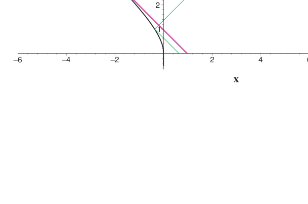
Figure 2:

6 The Story of Temperature

In what follows I adopt Unruh’s definition of a thermometer; i.e., a quantum system with multiple energy levels interacting with the field $\phi(t,x)$. In other words, I add an interaction of the form

$$V_{\rm int}(t)=\epsilon\,e^{-(t-t_{0})^{2}/2\sigma}Q\,\phi(x,t)$$ (23)

to the Lagrangian, where the parameters $t_{0}$ and $\sigma$ define the range in $t$ for which the interaction is turned on and $x$ specifies the spatial location of the thermometer. Furthermore, the operator $Q$ is some operator causing transitions among the energy eigenstates of the thermometer.

Of course, assumptions have to be made in order to get reasonable results. First, in order for the thermometer to know the mirror is moving, it is necessary that $t_{0}>>x$. Second, we impose an adiabatic condition, $\sqrt{\sigma}>>1/E$, where $E$ is the typical excitation energy of the thermometer, so that we do not excite the termometer just by turning it on or off. Finally, we impose the condition $E\sim\kappa$, so that the acceleration of the mirror is capable of exciting the higher states of the thermometer.

With these assumptions second order perturbation theory in $\epsilon$ tells us that the probability of the thermometer being excited to a state with energy $E$ is

$${\cal P}(E,E_{0}) = \epsilon^{2}|\langle{E}|M(0)|{E_{0}}\rangle|^{2}\int dt\,dt^{\prime}$$ (24)

$$e^{-i(E-E_{0})(t-t^{\prime})}e^{-(t-t_{0})^{2}/2\sigma}$$

$$e^{-(t^{\prime}-t_{0})^{2}/2\sigma}\langle\phi(t,x)\,\phi(t^{\prime},x)\rangle$$

What we now do is compute $\langle\phi(t,x)\,\phi(t^{\prime},x)\rangle$ by plugging in the formula giving $\phi(t,x)$ in terms of $\phi(x)$ and $\pi(x)$ on the original surface, expand these $t=0$ operators in terms of annihilation and creation operators and evaluate the resulting expression. The key feature of this problem is that the points on the original surface corresponding to $(t,x)$ and $(t^{\prime},x)$ for $t,t^{\prime}>>x$ are exponentially close to the point $x=A$. A straightforward computation gives the result

$${\cal P}(E,E_{0}) = {\epsilon^{2}\sqrt{\pi}\over 2}\,{|\langle{E}|M(0)|{E_{0}}\rangle|^{2}\over E-E_{0}}$$

$$\times \left[{1\over e^{2\pi\,(E-E_{0})/\kappa}-1}\,\right]$$ (25)

7 Computing The Energy Flux

To compute the flux of energy through a plane at position $x$ we need to compute $T_{tx}$, the energy momentum tensor for the massless field, which is given by

$$T_{\mu\nu}={1\over 2}\left\{\partial_{\mu}\phi(t,x),\partial_{\nu}\phi(t,x)\right\},$$ (26)

Generally, the expectation value of components of $T_{\mu\nu}$ will be divergent since the field derivatives are being evaluated at the same spacetime point. To deal with this we adopt a point splitting procedure; i.e., we define

$$T_{tx}={1\over 2}\left\{\pi(t+\delta,x),\partial_{x}\phi(t-\delta,x)\right\},$$ (27)

evaluate the expression and then take the limit $\delta\rightarrow 0$. The result is that the energy density $T_{tt}$ diverges as $1/\delta^{2}$ but the flux, $T_{tx}$, is finite and unique. The result of the computation is

$$T_{tx}={\kappa^{2}\over 48\pi}$$ (28)

Although the finiteness of the flux may seem surprising, it is in fact a consequence of a general theorem.

8 The Black Hole

Now let us turn to a discussion of the case of a Schwarzschild black hole. Another way of describing the previous example is to say that we solve the Heisenberg equations by tracing back the two null-rays leaving the point $(t,x)$ to find the two points at which they intersect the $t=0$ surface and write the field in terms of the $\phi$ and $\pi$ at those two points. There is a simple generalization of this approach to the equations in curved space.

Straightforward analysis shows that what is usually referred to as a WKB analysis of the wave equation in curved space amounts to, what we will call, the Geometric Optics Approximation. The generalization is given by the following prescription. First, starting from the point $(\lambda,r)$, find the two null-geodesics which meet at this point and trace them back to the surface $\lambda=0$ (since this is a geometrical statement it can be solved in any coordinate system). In Painlevé coordinates the equations for these two geodesics are

$$S_{1}(x_{1}) = \lambda+S_{1}(r)$$

$$S_{2}(x_{2}) = \lambda+S_{2}(r)$$

$$S_{1}(r) = r-2\sqrt{r}+\ln((\sqrt{r}+1)^{2})$$

$$S_{2}(r) = -r-2\sqrt{r}-\ln((\sqrt{r}+1)^{2})$$ (29)

Next, having found the points $x_{1}$ and $x_{2}$, write the field at $(\lambda,r)$ as

$$\phi(\lambda,r)={1\over r}\left(\phi_{1}(\lambda+S_{1}(r))+\phi_{2}(\lambda+S_{2}(r))\right)$$ (30)

where the field on the initial surface is given in terms of two functions

$$\phi(0,r) = {1\over r}\left(\phi_{1}(S_{1}(r))+\phi_{2}(S_{2}(r))\right)$$ (31)

$$= {1\over r}\left(f_{1}(r)+f_{2}(r)\right)$$

Finally, in analogy with the flat space case, write $f_{1}$ and $f_{2}$ in terms of $\phi(r)$ and $\pi(r)$ on the surface of quantization ($\lambda=0$).

9 Black Hole: Thermometer Redux

Let us now consider adiabatically switching on a thermometer, kept at fixed Schwarzschild $r$, and then switching it off. As in the case of the moving mirror, second order perturbation says

$${\cal P}(E,E_{0}) = \epsilon^{2}|\langle{E}|M(0)|{E_{0}}\rangle|^{2}\int d\lambda\,d\lambda^{\prime}$$ (32)

$$e^{-i(E-E_{0})(\lambda-\lambda^{\prime})}e^{-(\lambda-\lambda_{0})^{2}/2\sigma}$$

$$e^{-(\lambda^{\prime}-\lambda_{0})^{2}/2\sigma}\langle\phi(\lambda,r)\,\phi(\lambda^{\prime},r)\rangle$$

Of course, now the points $(\lambda,r)$ and $(\lambda^{\prime},r)$ in the correlation function $\langle\phi(\lambda,r)\phi(\lambda^{\prime},r)\rangle$ are traced back, using null-geodesics, to the initial surface $\lambda=0$ and the fields are appropriately re-expressed in terms of $\phi$ and $\pi$ on that surface. The only subtlety in this calculation is that for arbitrary $r$ the interaction term gets an extra correction for the time dilation at point $r$, since the energy levels of the thermometer are defined in its rest frame. The result of this calculation is that the thermometer reads a temperature

$$k_{B}\,T={1\over 8\pi M\sqrt{1-2M/r}}$$ (33)

which agrees with Hawking’s result.

10 Black Hole: Energy Flux

The energy flux for the Schwarzschild black hole is calculated in the same way as for the moving mirror. Again we have to point-split the fields appearing in the energy momentum tensor and then take the limit of zero splitting. As before we find that the flux $T_{\lambda,r}$ is finite and the total flux through a sphere at large $r$ takes the expected limiting value

$${\rm Flux}={\pi\over 12}\ T^{2}={\pi\over 12}\ {1\over(8\pi M)^{2}}$$ (34)

plus, of course, transients which vanish for large $\lambda$ and terms which die faster than $1/r^{2}$.

11 Back Reaction

Our approach is unique in that we start at a finite time and calculate everything as a function for all values of $\lambda$ and $r$. Thus, in principle, one can discuss the problem of back reaction after the Hawking radiation has set in, but before any appreciable amount of the black hole’s mass has been radiated. The reason there is a back reaction problem is because we calculated the energy-momentrum tensor for a Schwarzschild background and found a non-vanishing $T_{\lambda r}$ and so we are in the situation that

$$G_{\mu\nu} = R_{\mu\nu}-g_{\mu\nu}\,R=0$$

$$T_{\mu\nu} \neq 0.$$ (35)

This, of course, is not consistent with the Einstein equations and so we do not have a self-consistent semi-classical problem.

Given our computational procedure, however, for any point $r$, $T_{\lambda r}$ is zero until radiation from the horizon has a chance to reach that point, at which time an observer begins to see the Hawking radiation. In principle we could feed our expression for $T_{\mu\nu}$ back into the Einstein equations and attempt to find a self-consistent metric for which the computation of $T_{\mu\nu}$ wouldn’t change very much. Clearly this is difficult to do in general but we can ask what things look like inside of a sphere of radius $r$ after the Hawking radiation has set in. If, in this region we adopt a metric of Schwarzschild form but change $M$ to $M(t)=M_{0}-Ft$ then the metric becomes

$$ds^{2} = -(1-{2M(t)\over r})\,dt^{2}+{1\over(1-{2M(t)\over r})}\,dr^{2}$$ (36)

$$+r^{2}d\Omega^{2}$$

which leads to an Einstein tensor of the form

$$\pmatrix{0&{2\,F\over r^{2}X(t)}&0&0\cr{2\,F\over r^{2}\,X(t)}&0&0&0\cr 0&0&{4\,F^{2}\over X(t)^{3}}&0\cr 0&0&0&{4\,F^{2}\sin(\theta)^{2}\over X(t)^{3}}\cr}$$ (37)

where

$$X(t)=1-{2\,(M_{0}-F\,t)\over r}$$ (38)

which matches the outgoing flux computed for the static background. Since our computation of the flux at a point $(t,r)$ only involves the computation of geodesics leaving the initial surface and arriving at this point. It is clear that for a large black hole these geodesics will not change very much for time intervals for which the Hawking radiation has set in but during which only a neglible fraction of the black hole mass has been radiated away. Therefore, it would seem that an iterative self-consistent solution should be possible.

12 Entropy?

While the two issues of entropy and the issue of decoupling of modes at $r=0$ are very interesting, there is no time to discuss them in this talk. A discussion of these issues will appear in a forthcoming paper.

References

- [1] Kirill Melnikov and Marvin Weinstein, hep-th/0109201 (2001),
- [2] S. W. Hawking, Commun. Math. Phys. 43, 199 (1975); J.B. Hartle and S.W. Hawking, Phys. Rev. D13, 2188 (1976).
- [3] W.G. Unruh, Phys. Rev. D14, 870 (1976).
- [4] T. Jacobson and D. Mattingly, Phys. Rev. D61, 024017 (2000).
- [5] M. Parikh and F. Wilczek, Phys. Rev. Lett. 85, 5042 (2000).
- [6] If the initial state is not the vacuum state but any finite energy state of the instantaneous Hamiltonian, the finite energy will be radiated away in finite amount of time. The structure of radiation at large later times is independent of the initial quantum state of the massless field.
- [7] N.D. Birrell and P.C.W. Davies, Quantum Fields in the curved space, Cambridge University Press, 1984.
- [8] B.S. DeWitt, in General Relativity, eds. S.W. Hawking and W. Israel, Cambridge University Press, 1979.