Gravitational radiation from the $r$-mode instability

Abstract

The instability in the $r$-modes of rotating neutron stars can (in principle) emit substantial amounts of gravitational radiation (GR) which might be detectable by LIGO and similar detectors. Estimates are given here of the detectability of this GR based the non-linear simulations of the $r$-mode instability by Lindblom, Tohline and Vallisneri. The burst of GR produced by the instability in the rapidly rotating 1.4$\,M_{\odot}$ neutron star in this simulation is fairly monochromatic with frequency near $960\,$Hz and duration about $100\,$s. A simple analytical expression is derived here for the optimal $S/N$ for detecting the GR from this type of source. For an object located at a distance of $20\,$Mpc we estimate the optimal $S/N$ to be in the range $1.2\sim 12.0$ depending on the LIGO II configuration.

1 Introduction

This paper contains a portion of the material presented by Lee Lindblom in the talk “Relativistic Instabilities in Compact Stars” at the Fourth Amaldi Conference on Gravitational Waves. Most of the material presented in that talk has already been published, and so we limit our discussion here to that material which has not previously appeared in print. We direct those readers who might be interested in the wider range of subjects covered in the talk to the recent review Lindblom (2001), and the recent papers Lindblom, Tohline and Vallisneri (2001b) and Lindblom and Owen (2001).

Gravitational radiation (GR) is a de-stabilizing force on the $r$-modes of rotating neutron stars (Andersson 1998, Friedman and Morsink 1998). The first estimates of the timescales associated with this instability (Lindblom, Owen and Morsink 1998) showed that the GR driving force is much stronger than the stabilizing effects of the simplest forms of viscous dissipation in neutron stars. As a consequence there has been a great deal of interest in this instability as a potential source of observable GR, and as a mechanism for removing angular momentum from rapidly rotating neutron stars. During the past several years the effects of a number of additional dissipation mechanisms on the $r$-mode instability have been studied in some detail. A number of these mechanisms are much more effective in suppressing the $r$-mode instability than the simple viscosity considered in the initial estimates. In particular the effects of a solid crust (Bildsten and Ushomirsky 2000, Lindblom, Owen and Ushomirsky 2000, Wu, Matzner and Arras 2001), the effects of magnetic fields (Rezzolla, et al2001a, 2001b, Mendell 2001), the non-linear effects of mode-mode coupling (Schenk, et al2001), and the effects of hyperon bulk viscosity (Jones 2001a, 2001b, Lindblom and Owen 2001) make it appear less likely that the GR instability in the $r$-modes will play an interesting role in astrophysics. However, at the present time none of these mechanisms is understood well enough for us to conclude absolutely that the $r$-mode instability will never play a role in any neutron stars. Thus for the purposes of the present paper, we assume that the instability will occur in some rapidly rotating neutron stars. Our aim here is to present the best estimate of the GR that might be emitted during such an instability. To do this we analyze the GR emitted by the best currently available numerical simulation of the non-linear evolution of the $r$-mode instability. This paper is an update of the initial estimates of the GR emitted by the $r$-mode instability given by Owen, et al(1998).

2 r-Mode Evolution Model

We base our estimates of the GR produced by the non-linear evolution of an unstable $r$-mode, on the numerical simulations by Lindblom, Tohline and Vallisneri (2001a, 2001b). The evolution of a small amplitude $m=2$ $r$-mode subject to the current-quadrupole GR reaction force was studied numerically in a $1.4M_{\odot}$ polytropic neutron star rotating at about 95% of its breakup angular velocity. Figure 1 illustrates the evolution of the current quadrupole moment $|J_{22}|$ (in cgs units) of this model as the simulation evolves. The current quadrupole moment is defined as

$$J_{22}=\int\rho r^{2}\vec{v}\cdot\vec{Y}^{B*}_{22}d^{\,3}x,$$ (1)

where $\rho$ and $\vec{v}$ are the density and velocity of the fluid in the star, and $\vec{Y}^{B}_{22}$ is the magnetic type vector spherical harmonic (Thorne 1980). The time displayed along the horizontal axis of Fig. 1 is given in units of the initial rotation period of the star: $P_{0}=1.18\,$ms. During the first part of the evolution GR drives the growth of the $r$-mode, leading to the exponential growth in $J_{22}$ illustrated here. Once the amplitude of the mode becomes sufficiently large, however, non-linear hydrodynamic processes also become important. These lead to large surface waves which break and shock (see Lindblom, Tohline and Vallisneri 2001a, 2001b). The dissipation in these shocks damps the $r$-mode and leads to the rapid decrease in $J_{22}$ following its peak.

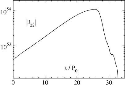
Figure 1: Evolution of the current quadrupole moment $J_{22}$ (in cgs units) from the numerical simulation of the GR driven growth of the $m=2$ $r$-mode.

The timescale of the GR instability in the $r$-modes is much much longer than the hydrodynamic timescale. To perform the numerical simulation illustrated in Fig. 1 it was necessary to increase artificially the strength of the GR driving force so that the instability could proceed more rapidly. Fortunately tests have shown (see Lindblom, Tohline and Vallisneri 2001b) that the maximum amplitude which the $r$-mode achieves (and hence the maximum value of $J_{22}$) is relatively insensitive to the strength of the GR driving force. The amplitude grows until the velocities in the mode reach some critical value before the waves break and shock. The value of this critical velocity appears to be relatively insensitive to how rapidly the fluid velocity is increased to this critical level.

To determine the GR signal that would be emitted by the growth of an unstable $r$-mode, it is necessary to re-scale the time in the simulation. The early part of the simulation has been designed to proceed more rapidly than the physical case by the factor $\tau_{GR}({\rm physical})/\tau_{GR}({\rm simulation})$, where $\tau_{GR}$ represents the GR growth timescale of the instability. This ratio has the value 4488 in the simulation used here. Thus the early exponential growth phase of a physical $r$-mode evolution will last longer than this phase of the simulation by this factor. The late stages of the simulation are dominated by hydrodynamic forces which damp the $r$-mode within a few rotation periods. This final stage of the evolution therefore proceeds at the same rate in both the physical and the simulation cases. We (somewhat artificially) choose the dividing time between the early and late stages of the evolution to be the time at which the value of $|J_{22}|$ is maximum.

The time dependence of $J_{22}$ is found in the simulation to be nearly sinusoidal with a time dependent amplitude, $J_{22}=|J_{22}|e^{i\psi(t)}$, (with $d\psi/dt=\omega\approx$ constant) because $J_{22}$ is dominated by the unstable $r$-mode in this case. The time dependence of $|J_{22}|$ is illustrated in Fig. 1. The frequency of the sinusoidal time dependence is conveniently determined numerically using the formula

$$\omega=-{1\over|J_{22}|}\left|{dJ_{22}\over dt}\right|.$$ (2)

This approximation introduces errors of order $(\omega\tau_{GR})^{-1}\approx 2\%$ in our simulation. Figure 2 illustrates the evolution of the frequency, $f=-2\pi\omega$, determined numerically in this way. Here we plot the frequency as a function of the re-scaled physical time (in seconds). We note that the frequency changes by only a few percent during the course of the evolution in which about 40% of the angular momentum of the star is radiated away as GR.

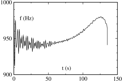
Figure 2: Evolution of the “frequency” of the $r$-mode. The time parameter used here (in seconds) is scaled from the simulation to reflect the physical case until the formation of shocks. Noise early in the simulation is due to contamination of the current quadrupole $J_{22}$ by other modes.

In general relativity theory an isolated object with time dependent current quadrupole moment radiates GR. The expression for the dimensionless GR amplitude $h$ (averaged over possible source and detector orientations) is given by

$$h(t)=\frac{16}{15}\sqrt{\frac{2\pi}{5}}\frac{\omega^{2}G|J_{22}|}{c^{5}D}e^{i\psi(t)},$$ (3)

where $G$ and $c$ are Newton’s constant and the speed of light, and $D$ is the distance to the source. Figure 3 illustrates the time dependence of this dimensionless GR amplitude as a function of time as determined by the simulation. Since the frequency of these $r$-mode oscillations is essentially constant, the GR amplitude just grows in proportion to $J_{22}$. Once the amplitude peaks, non-linear hydrodynamic forces (i.e. shocks) quickly damp the mode and this is reflected in the sharp drop in $h$ (as a function of physical time) illustrated in Fig. 3. We have chosen $D=20\,$Mpc, the distance to the Virgo Cluster of galaxies, for the purposes of the illustration. Optimistic estimates of the event rate for these objects suggests that the nearest events expected during the time frame of the LIGO observations will be at this distance.

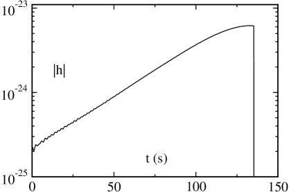
Figure 3: Evolution of the angle averaged dimensionless gravitational wave amplitude $|h(t)|$ for a source located at a distance $D=20\,$Mpc. The time parameter used here (in seconds) is scaled from the simulation to reflect the physical case until the formation of shocks.

3 Optimal S/N

The optimal signal to noise ratio ($S/N$) for detecting a GR signal can be achieved with the use of an optimal filter, consisting of a template that matches the waveform of the signal. Let $\tilde{h}$ denote the Fourier transform of the GR signal:

$$\tilde{h}(f)=\int_{-\infty}^{\infty}h(t)e^{-2\pi ift}dt.$$ (4)

The discrete Fourier transform of the gravitational wave signal from our numerical simulation is shown in Fig. 4. Here we have smoothed the resulting $|\tilde{h}(f)|^{2}$ with a windowing function of width $0.5\,$Hz. We see that the spectrum of the gravitational radiation is confined essentially to the band $940\leq f\leq 980\,$Hz, which corresponds well with the evolution of the frequency of the $r$-mode as shown in Fig. 2. For a complex signal $h(t)$ the optimal value of $S/N$ is given by

$$\left(\frac{S}{N}\right)^{2}=2\int_{0}^{\infty}\frac{|\tilde{h}(f)|^{2}df}{S_{h}(f)},$$ (5)

where $S_{h}(f)$ is the one-sided power spectral density of detector noise. (For a real signal the 2 becomes a 4.) We approximate $S_{h}(f)$ for frequencies near $960\,$Hz by the Taylor expansion

$$S_{h}(f)\approx S+S^{\prime}\Delta f+0.5S^{\prime\prime}(\Delta f)^{2},$$ (6)

where $\Delta f=f-960\,$Hz, and the three constants $S$, $S^{\prime}$ and $S^{\prime\prime}$ are listed in Table 1 for three plausible LIGO II design options (see Buonanno and Chen 2001). Using these values for $S_{h}$ we find $S/N\approx 1.2$, 4.0 and 10.4 by performing the integral in Eq. (5) numerically for these three possible LIGO II configurations.

Table 1: Coefficients for the Taylor expansion of the one-sided power spectral density $S_{h}$ at $f=960\,$Hz for three plausible LIGO II configurations.

• Configuration		$\quad S$		$\quad S^{\prime}$		$\quad S^{\prime\prime}$
  NS–NS Optimized	$2.$	$0\times 10^{-46}\,$Hz-1	$5.$	$0\times 10^{-49}$ Hz-2	$5.$	$6\times 10^{-52}\,$Hz-3
  Broadband	$1.$	$9\times 10^{-47}\,$Hz-1	$2.$	$2\times 10^{-50}$ Hz-2	$2.$	$6\times 10^{-53}\,$Hz-3
  Narrowband	$2.$	$7\times 10^{-48}\,$Hz-1	$6.$	$0\times 10^{-51}$ Hz-2	$8.$	$1\times 10^{-52}\,$Hz-3

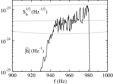
Figure 4: Fourier transform of the gravitational wave amplitude illustrated in Fig. 3, $|\tilde{h}(f)|$. Also shown are the noise power spectral density $S^{1/2}_{h}$ for the three potential LIGO II configurations used in our estimates of the optimal $S/N$.

We can also make an analytical estimate of the optimal $S/N$ using an extension of a very general argument given originally by Blandford (1984, unpublished). For GR emitted by a multipole with azimuthal quantum number $m$ the angular momentum loss rate is

$$\frac{dJ}{dt}=-\frac{5m\pi c^{3}}{2G}fD^{2}|h(t)|^{2},$$ (7)

where $|h(t)|^{2}$ has been averaged over all possible orientations of source and detector (and over several wave periods for the case of a real signal). When a function such as $h(t)$ involves a rapid oscillation together with a much slower evolution of its amplitude and frequency, the Fourier transform $\tilde{h}(f)$ is well approximated by the stationary phase approximation,

$$|h(t)|^{2}=|\tilde{h}(f)|^{2}\left|\frac{df}{dt}\right|$$ (8)

for a complex signal $h(t)$. (For a real signal, the left-hand side is averaged over several periods and the right-hand side is multiplied by 2.) Since the angle-averaging affects both sides of Eq. (8) equally, we can use Eqs. (7) and (8) to re-express $S/N$ for a source at an “average” orientation from Eq. (5) as

$$\left(\frac{S}{N}\right)^{2}=-\frac{4G}{5m\pi c^{3}D^{2}}\int\frac{dJ}{fS_{h}(f)}.$$ (9)

For GR sources such as the $r$-mode evolution the frequency of the radiation emitted is nearly constant, so $fS_{h}(f)$ can be treated as being essentially constant in Eq. (9). Thus, this integral becomes just the total amount of angular momentum $\left|\Delta J\right|$ radiated away as GR:

$$\left(\frac{S}{N}\right)^{2}=\frac{4G}{5m\pi c^{3}D^{2}}\frac{\left|\Delta J\right|}{fS_{h}(f)}.$$ (10)

The total amount of angular momentum radiated away as GR in the simulation was $|\Delta J|\approx 4.5\times 10^{48}$ in cgs units. Using this value in Eq. (10) together with the values of $S_{h}$ from Eq. (6) and Table 1, we find $S/N\approx 1.4$, 4.5, and 12.0 in good agreement with our previous estimate based on the discrete Fourier transform and direct integration of the simulation waveform. We note that this argument can easily be extended to signals composed of multiple harmonics and multipoles so long as their frequencies are well-defined: Time-averaging of Eq. (8) eliminates cross-terms, so Eq. (10) is simply summed over each harmonic and $m$. We can also extend the argument to non-monotonically evolving frequencies by using Eq. (8) to express Eq. (5) as an integral over time and dividing $f(t)$ into piecewise monotonic parts.

It is not unreasonable to think that a realistic data analysis strategy could come within a factor of 2 of the optimal $S/N$. Due to the complexity of the physics involved it seems unlikely that matched filtering will ever be a viable option. However, cross-correlation of the output of two aligned interferometers (LIGO Hanford and LIGO Livingston) can in principle achieve $1/\sqrt{2}$ of optimal $S/N$ if the detectors’ noise is of comparable strength and uncorrelated—including non-Gaussian noise bursts (Anderson et al2001). This strategy relies on the supernova associated with the $r$-mode having been observed optically, allowing the appropriate time delay to be inserted between the interferometer data streams. Narrowing the search to a few minutes after the supernova (instead of continuous operation) also has the effect of greatly reducing the $S/N$ threshold for detection with reasonable false alarm statistics. Thus a cross-correlation with $S/N\approx 4$ might be considered enough for detection, implying a realistically detectable distance for $r$-modes of 5 Mpc for even the least optimal (for this type of source) LIGO II configuration—and up to 50 Mpc for the most optimal.

References

References

- [1]
- [2] [] Anderson W G, Brady P R, Creighton J D E and Flanagan É É 2001 Phys. Rev. D 63 042003
- [3]
- [4] [] Andersson N 1998 Astroph. J. 502 708
- [5]
- [6] [] Bildsten L and Ushomirsky G 2000 Astroph. J. 529 L33
- [7]
- [8] [] Buonanno A and Chen Y 2001 Phys. Rev. D 64 042006
- [9]
- [10] [] Friedman J L and Morsink S M 1998 Astroph. J. 502 714
- [11]
- [12] [] Jones P B 2001a Phys. Rev. Lett.86 1384
- [13]
- [14] [] Jones P B 2001b Phys. Rev. D 64 084003
- [15]
- [16] [] Lindblom L 2001 in Gravitational Waves: A Challenge to Theoretical Astrophysics, ed V Ferrari et al(Trieste: ICTP Lecture Notes, Vol 3) pp 257–275; http://www.ictp.trieste.it
- [17]
- [18] [] Lindblom L and Owen B J 2001 Phys. Rev. D (submitted); astro-ph/0110558
- [19]
- [20] [] Lindblom L, Owen B J and Morsink S M 1998 Phys. Rev. Lett.80 4843
- [21]
- [22] [] Lindblom L, Owen B J and Ushomirsky G 2000 Phys. Rev. D, 62, 084030
- [23]
- [24] [] Lindblom L, Tohline J E and Vallisneri M 2001a Phys. Rev. Lett.86 1152
- [25]
- [26] [] Lindblom L, Tohline J E and Vallisneri M 2001b Phys. Rev. D (submitted); astro-ph/0109352
- [27]
- [28] [] Mendell G 2001 Phys. Rev. D 64 044009
- [29]
- [30] [] Owen B J, Lindblom L, Cutler C, Schutz B F, Vecchio A and Andersson N 1998 Phys. Rev. D 58 084020
- [31]
- [32] [] Rezzolla L, Lamb F L, Markovic D and Shapiro S 2001a Phys. Rev. D 64 104013
- [33]
- [34] [] Rezzolla L, Lamb F L, Markovic D and Shapiro S 2001b Phys. Rev. D 64 104014
- [35]
- [36] [] Schenk A K, Arras P, Flanagan E E, Teukolsky S A, Wasserman I gr-qc/ 0101092
- [37]
- [38] [] Thorne K 1980 Rev. Mod. Phys.52 299
- [39]
- [40] [] Wu Y, Matzner C D and Arras P 2001 Astrophys. J 549 1011
- [41]