Constraint-preserving boundary conditions in numerical relativity

Abstract

This is the first paper in a series aimed to implement boundary conditions consistent with the constraints’ propagation in 3D unconstrained numerical relativity. Here we consider spherically symmetric black hole spacetimes in vacuum or with a minimally coupled scalar field, within the Einstein-Christoffel (EC) symmetric hyperbolic formulation of Einstein’s equations. By exploiting the characteristic propagation of the main variables and constraints, we are able to single out the only free modes at the outer boundary for these problems. In the vacuum case a single free mode exists which corresponds to a gauge freedom, while in the matter case an extra mode exists which is associated with the scalar field. We make use of the fact that the EC formulation has no superluminal characteristic speeds to excise the singularity.

We present a second-order, finite difference discretization to treat these scenarios, where we implement these constraint-preserving boundary conditions, and are able to evolve the system for essentially unlimited times. As a test of the robustness of our approach, we allow large pulses of gauge and scalar field to enter the domain through the outer boundary. We reproduce expected results, such as trivial (in the physical sense) evolution in the vacuum case (even in gauge-dynamical simulations), and the tail decay for the scalar field.

I Introduction and overview

In the initial value problem of Einstein’s equations one decomposes the original system of equations (given by $G_{ab}=8\pi T_{ab}$) into two distinct sets: one set consisting of evolution equations (involving time derivatives of the main variables) and the other consisting of constraint equations (which do not involve time derivatives). There are infinite possible ways of achieving this decomposition, and the resulting systems are known by a variety of different names (e.g. ADM, characteristic-Bondi and conformal-Einstein approaches, to name just three). However, depending on the character of the hypersurfaces used to foliate the spacetime, these formulations can be seen as belonging to different groups: the group of Cauchy formulations (which require a spacelike foliation), that of characteristic formulations (having a null foliation), or a more generic group (where the foliation’s leaves need not have a fixed specific character) (see, for instance, [1]).

Irrespective of the group and restricting to the initial value problem (where the problem is boundary-free), the state of the system is defined at an initial hypersurface $\Sigma_{0}$ and the solution to the future of $\Sigma_{0}$ is obtained through the evolution equations. However, if the system of equations involves constraints, one might opt to employ only a subset of the evolution equations supplemented with enough constraint equations to solve for the field variables. This strategy is referred to as constrained evolution, as opposed to free evolution (where only the evolution equations are employed). In the particular case of Einstein’s equations, a straightforward manipulation of the Bianchi identities demonstrates that either strategy produces, at the analytical level, the same solution. Therefore, one need not deal with constrained evolution (which usually requires solving elliptic equations) and the more direct approach of free evolution can be safely employed. In the numerical realm, however, the picture is more complicated (for definiteness, from now on we concentrate on the case of Cauchy evolution). On one hand, employing constrained evolutions might represent a significant computational overhead as it usually involves solving elliptic equations at each time step; for this reason constrained evolutions have been, for the most part, avoided beyond the two-dimensional case. On the other hand, free evolution in numerical implementations (which only evaluate the constraint equations to monitor the quality of the implementation) display violation of the constraints. At early times, these violations are consistent with the truncation error [2], but as time progresses the observed violations often grow quite rapidly.

The picture gets even more complicated in the presence of boundaries. The violation of the constraints in unconstrained numerical evolutions frequently grows without bound. Possible reasons, besides the ones already present in boundary-free models, are constraint-violating modes introduced by standard boundary conditions (which might drive instabilities, and in any case do introduce spurious errors that should be avoided). If the case under study corresponds to cosmological scenarios or short term evolutions, the aforementioned problem should not be worrisome. In the cosmological case one has no boundaries (or rather, periodic boundary conditions are specified, which trivialize the specification issue), for solutions which are restricted to the future domain of dependence of the initial data no boundary conditions need be specified, and for short-term evolutions the errors introduced by approximate boundary conditions are restricted to a small region. There are, however, many non-cosmological important problems that require long term evolutions and hence the need to prescribe consistent boundary conditions; among these, collapse scenarios and black hole spacetimes.

In the one-dimensional case, approximate boundary conditions that minimize the influence of errors introduced at the boundary have been presented [3]. This is achieved by placing the boundaries far away and treating a region close to them in a special way (to control spurious reflections). Unfortunately, these techniques are not as effective in higher dimensional scenarios, as the computational cost involved in placing boundaries far away is excessive. Furthermore, even when there were enough computational resources, it would be preferable to make use of them to achieve finer resolved simulations, rather than to push boundaries farther away. It is therefore of considerable importance to formulate relatively inexpensive boundary conditions whose associated errors do not depend on the boundaries’ locations, minimize spurious reflections, and guarantee that constraint-violating modes are not introduced.

Essentially, one aims to provide boundary conditions such that there is not only a unique solution to the evolution equations, but there is also preservation of the constraints throughout the computational domain. In a strongly hyperbolic formulation of gravity (see [4] for reviews on hyperbolic techniques applied to Einstein’s equations) the first requirement amounts to giving boundary conditions only to the characteristic modes that enter the computational domain at any given boundary. Satisfying the second requirement is considerably more involved and has only very recently started receiving attention. In the analytical realm, well posedness of the initial boundary value problem (for a particular system) has been established in [5], which sheds light on the physical understanding of the issue and shows that, at least in a by-case basis, the problem might be analytically tractable. In the numerical realm, several efforts (restricted to different scenarios) have illustrated the advantages of providing boundary conditions through the use of constraints [6]. It is precisely this problem that we want to address here within the context of Cauchy, unconstrained evolution.

The present work aims to contribute to the area with the particular motivation of addressing issues proper of numerical implementations. Although in this first paper we restrict our analysis to the spherically symmetric case and a particular way of reformulating Einstein’s equations, the procedure is straightforward to implement within any hyperbolic formulation of gravity and in three dimensions (3D).

We present a detailed discussion of the analytic treatment for the boundary conditions and illustrate its benefits with a simple numerical implementation which accurately evolves a spherically symmetric spacetime, stationary or dynamical (the dynamics either corresponding to gauge modes in the vacuum case or to true dynamics in the case of a minimally coupled scalar field), for unlimited periods of time and without sign of instabilities. Throughout this work we minimize the use of techniques specifically developed for treating spherically symmetric spacetimes, both analytical and numerical, to expedite the generalization to the 3D case.

Our starting point is the assumption that we are dealing with a first-order, quasilinear strongly hyperbolic formulation for Einstein’s equations. In the spherically symmetry case such a system can be written as $\dot{u}=Au^{\prime}+l.o.$, where $u$ is an array of variables, dot and prime indicate time and spatial derivatives, respectively, $A$ (called the principal part) is a diagonalizable matrix that might depend on $u$ and the spacetime coordinates, but not on derivatives of $u$, and $l.o.$ stands for lower order terms, i.e. terms that do not have derivatives (of any kind). So, we have a system of equations for the main variables,

$$\dot{u}=Au^{\prime}+l.o.\;\;\;\mbox{(System I)}\;,$$ (1)

and evolution for the constraints, which we assume are also strongly hyperbolic,

$$\dot{u}_{c}=A_{c}u_{c}^{\prime}+l.o.\;\;\;\mbox{(System II)}\;.$$

If one were interested only in system I, one would give initial data for the variables that form $u$, and boundary data only to the ingoing characteristic modes. These characteristic modes (eigenvectors of $A$) are, depending on which boundary one is dealing with, the ones that are travelling to the left (positive eigenvalues) or right (negative eigenvalues).

A unique solution to system II is fixed, similarly, by giving initial data to $u_{c}$ and boundary conditions to the ingoing modes of the system. Since this is supposed to be an homogeneous system (which is the case in Einstein’s equations [7]), the identically zero solution is obtained by providing zero as initial data ($u_{c}=0$) and zero boundary conditions to the eigenmodes of $A_{c}$ entering the domain. The crucial point here is that, in unconstrained evolution, initial data and boundary conditions for $u_{c}$ follow from that of $u$. Thus, one has to provide initial and boundary data for $u$ such that they imply zero initial data and boundary conditions for $u_{c}$ (i.e. the data are consistent with all Einstein’s equations). The first step, namely, providing initial data that satisfy the constraints, is customarily well satisfied as the constraint equations are employed in the determination of data for $u$ (see [8, 1] and references cited therein). It is the second step that is usually neglected. Here we concentrate on this problem with the goal of providing consistent data, whose associated error neither depends on the location of the boundaries nor on the total evolution length; rather its error will agree with the overall truncation error of the global implementation.

The main difficulty with this second step is that the constraints (and, therefore the eigenmodes of system II as well) involve spatial derivatives of the main variables. On the other hand, by controlling the (ingoing) characteristic modes of system I at the boundaries, one does not control the spatial derivatives needed to set the ingoing constraint modes to zero. One way around this (and the one we use here), is to trade spatial derivatives for time derivatives using system I. Consequently, enforcing the constraints at the boundary amounts to controlling some time derivatives. We will make this construction explicit later but, before proceeding further, some comments are appropriate (both issues certainly deserve further analysis):

• To our knowledge, there is no rigorous result guaranteeing that in any strongly hyperbolic formulation of Einstein’s equations this trading of spatial for time derivatives can be done.

• When performing the trading, one ends up with some conditions at the boundaries on some time derivatives of the main variables. One must find out whether these conditions can be fulfilled by controlling only the ingoing modes of system I (at the numerical level, conditions on the time derivatives are enough for the application of the method of lines [9]). Again, we know of no proof showing that this should be possible in a general case.

We here show how this inversion can be performed in the 1D case, and leave for a future paper a similar analysis in 3D linear gravity [10].

When dealing with black hole spacetimes, boundary conditions customarily refer to the outer boundary conditions, but one might also have inner boundaries. These constitute “holes” or “excised” regions from a given computational domain; the most widely considered are those where the excised region has been chosen so as to remove the singularities when dealing with black hole spacetimes (assuming the validity of cosmic censorship). In this case, a region inside the black hole is excised from the computational domain (Unruh, cited in[11]). This excision strategy introduces an inner boundary which, if chosen inside the black hole, should leave the region outside the event horizon unaffected. Mathematically, the realization of this idea is ensured by employing a hyperbolic formulation with no superluminal characteristic speeds and, in particular, where all eigenvalues describe modes propagating towards the inner boundary. The non-triviality of excision if one does not have a formulation with these properties is discussed in one of the appendixes.

In recent years, a number of re-formulations of Einstein’s equations with physical characteristic speeds have been presented [12, 13, 14]: Here we make use of one of them in our analysis, the so-called Einstein-Christoffel (EC) system [12] (note that any other would have been equally well suited - our choice is simply motivated by a comparison with available results [15]).

The organization of this paper is the following: in section II we present the equations for the EC system describing a spherically symmetric massless scalar field minimally coupled to gravity. In section III we describe how to give boundary conditions that preserve the constraints, while in section IV we present our numerical method to test the procedure. Numerical results are included in section V, and are divided into three classes: evolution of stationary slicings of a Schwarzschild black hole, evolution of dynamical slicings of the same spacetime, and evolution of a massless scalar field interacting with a black hole. In all cases the simulations can be followed for unlimited times, even using very moderate resolutions. We demonstrate the accuracy of our method by monitoring the mass of the black hole in the vacuum case and reproducing the known tail decay in the scalar field case. A particularly strong test of the robustness of the approach is presented by letting strong gauge or scalar field pulses enter the computational domain through the outer boundary (compare with standard outer boundary treatments, where conditions are obtained by requiring the geometry at the outer boundary to be close to flat or Schwarzschild spacetimes, i.e. quite the opposite from what we do here).

II Main evolution equations and propagation of the constraints

As often is the case in hyperbolic formulations of Einstein’s equations, the EC formulation uses “exact” (i.e. arbitrary but a priori specified) shift and exact densitized lapse (defined by $\alpha=Ng^{-1/2}$, where $g$ is the determinant of the three-metric and $N$ is the lapse). In the present work, and for the sake of maintaining a uniform notation, we will follow as much as possible the conventions of [15]. For example, we write $\tilde{\alpha}:=\alpha r^{2}\sin{\theta}$, and

$$ds^{2} = -N^{2}dt^{2}+g_{rr}(dr+\beta dt)^{2}+r^{2}g_{T}(d\theta^{2}+\sin^{2}{\theta}d\phi^{2})\;,$$

$$K_{ij} = K_{rr}dr^{2}+r^{2}K_{T}(d\theta^{2}+\sin^{2}{\theta}d\phi^{2})\;,$$

where all fields depend only on $(t,r)$. Since the EC formulation is a first-order reformulation of Einstein’s equations, besides the three metric and extrinsic curvature, further variables (which basically contain information of spatial derivatives of the three-metric) are needed. In our present case of spherical symmetry, only two new variables require introduction, $f_{rrr}$ and $f_{rT}$, defined by

$$f_{rrr} = \frac{g_{rr}^{\prime}}{2}+\frac{4g_{rr}f_{rT}}{g_{T}}\;,$$

$$f_{rT} = \frac{g_{T}^{\prime}}{2}+\frac{g_{T}}{r}\;.$$

Additionally, we plan to study a scalar field $\Psi$ minimally coupled to the geometry. In order to re-express the equation that governs this field,

$$g^{ab}\nabla_{a}\nabla_{b}\Psi=0\;,$$

as a first-order hyperbolic system, we introduce two new variables:

$$\Pi := \frac{1}{\alpha}(\beta\Psi^{\prime}-\dot{\Psi})\;,$$

$$\Phi := \Psi^{\prime}\;.$$

The evolution equation for $\Psi$ decouples from the rest, in the sense that one has a closed system for the set of eight variables $(g_{rr},g_{T},K_{rr},K_{T},f_{rrr},f_{rT},\Pi,\Phi)$ which one can solve for, and afterwards obtain $\Psi$. Because of this, and following common practice, we will drop $\Psi$ from the system.

Thus, the main evolution equations, up to principal part (the complete expressions are listed in the appendix), are

$$\dot{g}_{rr}=\beta g^{\prime}_{rr}+l.o.\;,$$ (2)

$$\dot{g}_{T}=\beta g^{\prime}_{T}+l.o.\;,$$ (3)

$$\dot{K}_{rr}=\beta K^{\prime}_{rr}-\frac{N}{g_{rr}}f^{\prime}_{rrr}+l.o.\;,$$ (4)

$$\dot{K}_{T}=\beta K^{\prime}_{T}-\frac{N}{g_{rr}}f^{\prime}_{rT}+l.o.,\;,$$ (5)

$$\dot{f}_{rrr}=\beta f^{\prime}_{rrr}-NK^{\prime}_{rr}+l.o.\;,$$ (6)

$$\dot{f}_{rT}=\beta f^{\prime}_{rT}-NK^{\prime}_{T}+l.o.\;,$$ (7)

$$\dot{\Pi}=\beta\Pi^{\prime}-\frac{N}{g_{rr}}\Phi^{\prime}+l.o.\;,$$ (8)

$$\dot{\Phi}=\beta\Phi^{\prime}-N\Pi^{\prime}+l.o.\;.$$ (9)

The characteristic modes and eigenvalues determined by the system play a crucial role in our boundary treatment. These are (note that the modes with speed $\beta$ propagate along the timelike normal to the foliation, while the other modes propagate along the light cone),

$$u_{1}=g_{rr}\;\;\;(v_{1}=\beta)\;,$$ (16)

$$u_{2}=g_{T}\;\;\;(v_{2}=\beta)\;,$$

$$u_{3}=K_{rr}-g_{rr}^{-1/2}f_{rrr}\;\;\;(v_{3}=\beta+\tilde{\alpha}g_{T})\;,$$

$$u_{4}=K_{T}-g_{rr}^{-1/2}f_{rT}\;\;\;(v_{4}=\beta+\tilde{\alpha}g_{T})\;,$$

$$u_{5}=K_{rr}+g_{rr}^{-1/2}f_{rrr}\;\;\;(v_{5}=\beta-\tilde{\alpha}g_{T})\;,$$

$$u_{6}=K_{T}+g_{rr}^{-1/2}f_{rT}\;\;\;(v_{6}=\beta-\tilde{\alpha}g_{T})\;,$$

$$u_{7}=\Pi+g_{rr}^{-1/2}\Phi\;\;\;(v_{7}=\beta-\tilde{\alpha}g_{T})\;,$$

$$u_{8}=\Pi-g_{rr}^{-1/2}\Phi\;\;\;(v_{8}=\beta+\tilde{\alpha}g_{T})\;.$$ (17)

If we were dealing with a constraint-free system described by equations (2-9), a unique solution would be fixed by providing boundary conditions for the characteristic modes that are incoming at the boundaries and data on the initial hypersurface. However, we know that a solution to equations (2-9) is a solution of Einstein’s equations if and only if the following four constraints are also satisfied:

$$C:=\frac{f_{rT}^{\prime}}{g_{rr}g_{T}}-\frac{1}{2r^{2}g_{T}}+\frac{f_{rT}}{g_{rr}g_{T}}\left(\frac{2}{r}+\frac{7f_{rT}}{2g_{T}}-\frac{f_{rrr}}{g_{rr}}\right)-\frac{K_{T}}{g_{T}}\left(\frac{K_{rr}}{g_{rr}}+\frac{K_{T}}{2g_{T}}\right)+\frac{\Phi^{2}}{4g_{rr}}+\frac{\Pi^{2}}{4}=0,$$ (18)

$$C_{r}:=\frac{K_{T}^{\prime}}{g_{T}}+\frac{2K_{T}}{rg_{T}}-\frac{f_{rT}}{g_{T}}\left(\frac{K_{rr}}{g_{rr}}+\frac{K_{T}}{g_{T}}\right)+\Phi\Pi=0,$$ (19)

$$C_{rrr}:=g_{rr}^{\prime}+\frac{8g_{rr}f_{rT}}{g_{T}}-2f_{rrr}=0,$$ (20)

$$C_{rT}:=g_{T}^{\prime}+\frac{2g_{T}}{r}-2f_{rT}=0\;.$$ (21)

The first two are basically the Hamiltonian and momentum constraints, respectively, while the other two correspond to the definitions of the extra variables that make the system first order with respect to spatial derivatives. As mentioned, it is common practice to choose consistent initial data for Einstein’s equations by solving these constraints; however the constraints have been examined in a limited number of cases to provide consistent boundary data. The main purpose of this work is to provide further indications that constraints should be looked at more closely when dealing with boundary conditions. First, note that these constraints are defined in terms of the main variables, and a solution of the main evolution equations completely determines them as functions of spacetime. In particular, one can obtain the time evolution of the constraints by: (i) taking time derivatives of the right hand side (r.h.s.) of equations (18-21); (ii) replacing the time derivatives by the r.h.s. of equations (2-9); and, (iii) re-expressing the main variables in terms of the constraints and their spatial derivatives. In the present case, these are

$$\dot{C}=\beta C^{\prime}-\frac{N}{g_{rr}}C_{r}^{\prime}+l.o.\;,$$

$$\dot{C}_{r}=-NC^{\prime}+\beta C^{\prime}_{r}+l.o.\;,$$

$$\dot{C}_{rrr}=\beta C^{\prime}_{rrr}+l.o.\;,$$

$$\dot{C}_{rT}=\beta C^{\prime}_{rT}+l.o.\;.$$

We can also calculate the characteristic modes and eigenvalues of this system, obtaining:

$$C_{1}=C+g_{rr}^{-1/2}C_{r}\;\;\;(v^{c}_{1}=\beta-\tilde{\alpha}g_{T}),$$ (22)

$$C_{2}=C-g_{rr}^{-1/2}C_{r}\;\;\;(v^{c}_{2}=\beta+\tilde{\alpha}g_{T}),$$ (23)

$$C_{3}=C_{rrr}\;\;\;(v^{c}_{3}=\beta),$$ (24)

$$C_{4}=C_{rT}\;\;\;(v^{c}_{4}=\beta).$$ (25)

In the next section we exploit this information about the characteristic structure of our system in order to set up boundary conditions that will preserve the constraints at the boundaries.

III Constraint-preserving boundary conditions

In any system where the characteristic modes and eigenvalues are known, the data required at a given boundary are straightforwardly assessed by examining the eigenvalue of each characteristic mode. In our present case, these eigenvalues are $\lambda_{1}=\beta-\tilde{\alpha}g_{T}$, $\lambda_{2}=\beta+\tilde{\alpha}g_{T}$, and $\lambda_{3}=\beta$. In the case where the shift is exact, one can a priori guarantee which sign $\lambda_{3}$ will have. Throughout this paper we shall take $\beta$ as positive, since in that way we will be able to reproduce stationary known slicings of the Schwarzschild space-time, and to evolve dynamical spacetimes as well. The positivity of the shift implies that $\lambda_{2}$ is also positive. On the other hand, the sign of $\lambda_{1}$ depends on the solution and, thus, cannot be controlled a priori. However, for typical stationary slicings of Schwarzschild it is negative (positive) outside (inside) the black hole, and zero at the horizon. By continuity, the same will hold for (perhaps slight) distortions of these slicings. In our simulations we check numerically that this is indeed the case. As we shall see, even on highly distorted spacetimes this condition remains satisfied. Figure 1 shows a schematic diagram for the characteristic modes of a Schwarzschild black hole.

FIG. 1.: Schematic diagram for the characteristic speeds of the different modes in a stationary slicing of Schwarzschild black hole.

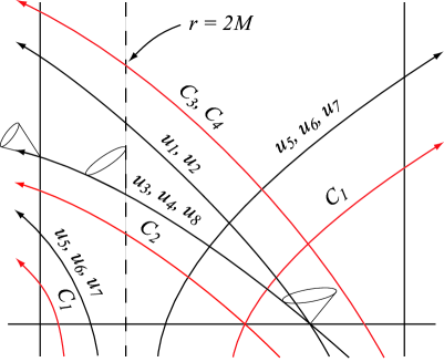
Our inner boundary is always inside the black hole, and no conditions are needed there. The usual procedure to make sure that the inner boundary is inside the hole is to track the apparent horizon. In spherical symmetry this is particularly simple since its location is defined in terms of algebraic combinations of the main variables ($f_{rT}-g_{rr}^{1/2}K_{T}=0$). Our actual procedure is to choose the initial data such that the inner boundary is inside the apparent horizon, and then numerically monitor its position during evolution. In our simulations the horizon never touches the inner boundary, so we do not need to move it, i.e. its grid location is fixed.

From the discussion in section II, we know that at the outer boundary (which in our case also has fixed grid location) we need to specify $u_{1},u_{2},u_{3},u_{4},u_{8}$ from the characteristic structure of the main equations. However, since the system is constrained, we are not free to choose these arbitrarily (which would be the case in an unconstrained system), but rather we must do so such that $C_{2}=C_{3}=C_{4}=0$ are satisfied (Note that $C_{1}$ is outgoing, therefore nothing special needs be done for it, nor should it be, otherwise we would overdetermine the constraint system of evolution equations.). This procedure, coupled with initial data satisfying the constraints, and the fact that the constraints are propagated with a quasilinear homogeneous system, will ensure that they are preserved everywhere.

We now make explicit how this procedure is implemented in our present case. We start by discussing how to enforce $C_{3}=C_{4}=0$ at the (outer, from now on) boundary. Writing down the constraints explicitly in equations (24,25), these conditions are

$$g_{rr}^{\prime}+\frac{8g_{rr}f_{rT}}{g_{T}}-2f_{rrr}=0,$$ (26)

$$g_{T}^{\prime}+\frac{2g_{T}}{r}-2f_{rT}=0\,.$$ (27)

Using equations (2,3), these can be rewritten as

$$\dot{g}_{rr} = 2g_{rr}\beta^{\prime}-2NK_{rr}-8\frac{g_{rr}f_{rT}}{g_{T}}\beta+2f_{rrr}\beta\ ,$$ (28)

$$\dot{g}_{T} = -2NK_{T}+2\beta f_{rT}\,.$$ (29)

Note that since $g_{rr}$ and $g_{T}$ correspond to ingoing modes, we are free to choose them such that they satisfy Eqs. (28,29). As was mentioned, one does not need to solve these two differential equations at the boundary, since time derivatives are all that is required for the time update in the method of lines, which we use for the time update (see section IV). Thus, we simply use the expressions (28,29) as the right hand side of the corresponding field variable at the boundary points (and similarly for $\dot{f}_{rT}$ and $\dot{K}_{T}$, see Eqs. (31, 32) below).

Lastly, $C_{2}=0$ needs to be enforced at the boundary. Using its definition, we have

$$\frac{1}{\sqrt{g_{rr}}}f_{rT}^{\prime}-K_{T}^{\prime}+l.o.=0\;.$$

Trading spatial for time derivatives, this in turn gives

$$\frac{1}{\sqrt{g_{rr}}}\dot{f}_{rT}-\dot{K}_{T}+l.o.=0\;.$$ (30)

Next observe that, by definition, $\dot{K}_{T}=\dot{K}_{T}(\dot{u}_{4},\dot{u}_{6},\dot{g}_{rr})$ and $\dot{f}_{rT}=\dot{f}_{rT}(\dot{u}_{4},\dot{u}_{6},\dot{g}_{rr})$. Since $\dot{g}_{rr}$ at the boundary is readily known from equation (28), Eq. (30) fixes the ingoing mode $\dot{u}_{4}$ (up to now free). From this, the definition of $u_{4}$ and $u_{6}$, and Eq. (28), we end with (recall that $u_{6}$ is outgoing, so it does not need boundary conditions)

$$\dot{f}_{rT}=\frac{g_{rr}^{1/2}}{2}\dot{u}_{6}+l.o.$$ (31)

$$\dot{K}_{T}=\frac{1}{2}\dot{u}_{6}+l.o.$$ (32)

Similarly, the ingoing mode $u_{3}$ is completely arbitrary. From it and the outgoing mode $u_{5}$ we have

$$K_{rr} = \frac{1}{2}(u_{3}+u_{5})\;,$$ (33)

$$f_{rrr} = \frac{g_{rr}^{1/2}}{2}(u_{5}-u_{3})\;.$$ (34)

Finally, the ingoing mode $u_{8}$ is also arbitrary. From it and the outgoing mode $u_{7}$ we have

$$\Pi = \frac{1}{2}(u_{7}+u_{8})\;,$$ (35)

$$\Phi = \frac{g_{rr}^{1/2}}{2}(u_{7}-u_{8})\;.$$ (36)

Equations (28,29,31,32,33,34,35,36) completely determine the boundary conditions for our eight variables; $u_{3}$ and $u_{8}$ are the only free modes. In the vacuum case, $u_{8}=0$ and $u_{3}$ describes a gauge mode.

In the next section we discuss our numerical implementation and results. One comment is in order before that: there is an additional constraint, $C_{matter}=\Phi-\Psi^{\prime}$, but by repeating the treatment described above one can see that this constraint fixes the boundary condition for $\Psi$: Since we are not evolving $\Psi$, we do not need to care about this.

IV Numerical simulations

To implement the proposed boundary treatment strategy, we have chosen a straightforward second-order dissipative method of lines. In particular, it was not necessary to employ techniques such as causal differencing [16], upwind discretization or any special way of treating the Lie-derived terms in Eqs. (2-9) (however, these can be readily incorporated as well). Spatial derivatives are discretized with second-order centered differences plus fourth-order dissipation as discussed in [17], while for the time integrator we use second-order Runge-Kutta (the dissipation added is, indeed, needed; otherwise, this method is unstable even for a simple scalar wave equation; see, e.g., [9]).

Our uniform grid structure consists of points $i=0\ldots N$, with grid spacing $\Delta r=L/N$, where $L=r_{outer}-r_{inner}$, and we implement derivatives according to standard formulae

$$Af^{\prime}\rightarrow AD_{0}f-\frac{\sigma_{i}}{\Delta t}(\Delta r)^{4}D_{+}D_{+}D_{-}D_{-}f\;,$$

$$(D_{0}f)_{i}=\frac{f_{i+1}-f_{i-1}}{2\Delta r}\;,$$

$$(D_{+}f)_{i}=\frac{f_{i+1}-f_{i}}{\Delta r}\;,$$

$$(D_{-}f)_{i}=\frac{f_{i}-f_{i-1}}{\Delta r}\;.$$

To evaluate derivatives at the boundaries, one either resorts to one-sided derivatives (which require different algorithms applied at boundary points) or introduces ghost zones, which are artificial points beyond the boundaries where field values are defined via extrapolation (one can choose the extrapolation order such that the answers from the different approaches are exactly the same). For convenience we chose the latter approach with only one ghost-zone for each boundary. Field values at these ghost zones are defined via third-order extrapolations and the same derivative operator is applied $\forall i,i=0..N$.

Since our inner boundary is always inside the black hole, we extrapolate all variables at the ghost zone point ($i=-1$).

At the outer boundary ghost zone ($i=N+1$), the outgoing modes $u_{5}$ and $u_{7}$ are also found by extrapolation, while the ingoing modes $u_{3}$ and $u_{8}$ are set as arbitrary functions of time. Next, equations (28,29,31,32) are integrated, at each time step, with second-order Runge Kutta. This, plus equations (33,34,35,36), completes the treatment for the outer boundary.

As a side note, it is worth mentioning that since we use only one ghost zone for each boundary, fourth-order derivatives cannot be obtained at the points $i=0,N$; thus, no dissipation is added to these points (we set $\sigma_{i=0}=\sigma_{i=N}=0$).

In all the cases discussed in this paper we have checked second-order self-convergence for the eight main variables, for the constraints and mass, as well as convergence with respect to the analytic solution, whenever this is available. The Courant-Friedrich-Levy factor $\lambda=\Delta t/\Delta r$ is set to $0.25$, and the dissipation factor is $\sigma_{i}=0.6/16$ (for $i=1..N-1$).

A Vacuum evolutions

1 Stationary slicing of a black hole

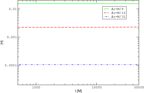
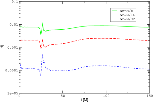
The simplest test of a black hole spacetime consists of reproducing known stationary slicings of a Schwarzschild black hole. For this test we give the corresponding known values both to the initial data and to the $u_{3}$ mode ($u_{8}$=0 for vacuum) at the outer boundary. We concentrate here on Painlevé-Gullstrand slicings, but we have obtained similar results using Kerr-Schild slicings. The code runs for unlimited times, even with resolutions as coarse as $\Delta r=M/6$ (with $M$ the mass of the black hole). Figure 2 displays the $L_{2}$ norm of the Hamiltonian constraint for three different resolutions and $L=9M$ ($r_{inner}=M$), the $L_{2}$ norm of a grid function $f$ being defined as

$$|f|:=\left(\frac{1}{L}\sum_{i=0}^{N-1}(f_{i})^{2}\Delta r\right)^{1/2}\;.$$

There is no growth in the Hamiltonian constraint, and the same holds true for the other three constraints.

FIG. 2.: $L_{2}$ norm of the Hamiltonian constraint, for the evolution of a Painlevé-Gullstrand black hole. In these runs the outer boundary is at $r=10M$.

FIG. 3.: $L_{2}$ norm of the relative mass error $|\delta M|=|{\cal M}-M|/M$, for the same runs shown in figure 2. After one thousand crossing times, the relative error for the coarsest resolution is around ten percent.

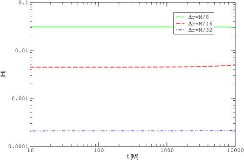
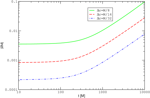
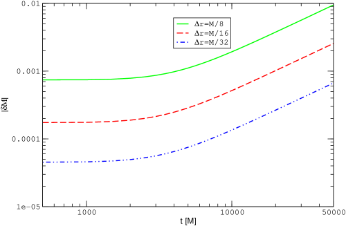
Figure 3 shows, for the same run, the $L_{2}$ norm of the relative error, $|\delta M|$, in the mass function ${\cal M}$, defined as

$$|\delta M|:=\frac{1}{M}|{\cal M}-M|\;,$$

where ${\cal M}$, the Misner-Sharp mass [18], is a gauge invariant [19] definition of the ADM mass $M$ in spherical symmetric vacuum:

$${\cal M}:=\frac{rg_{T}^{1/2}}{2}\left[1+\frac{r^{2}}{g_{T}}\left(K_{T}^{2}-\frac{f_{rT}^{2}}{g_{rr}}\right)\right]\;.$$ (37)

That is, each of the terms in the r.h.s. of Eq. (37) might be a function of $t$ and $r$, but Einstein’s vacuum equations in spherical symmetry imply that, at the continuum, the r.h.s.is a constant (equal to $M$), both as a function of space and time. When we compute $\delta M$ we evaluate ${\cal M}$ using the numerical values of the right hand side of Eq. (37), while for $M$ we use its analytical value.

From figure 3 we see that, as opposed to the constraints, there is a drift in the mass (this effect is expected, as second-order errors accumulate after many iterations) which, after a couple of hundred masses, is essentially linear in time.

FIG. 4.: Numerical value of the Misner-Sharp mass, scaled by its analytical value, as a function of radius, for different times. The monotonic behavior is explained by the fact that the black hole “moves” through the grid.

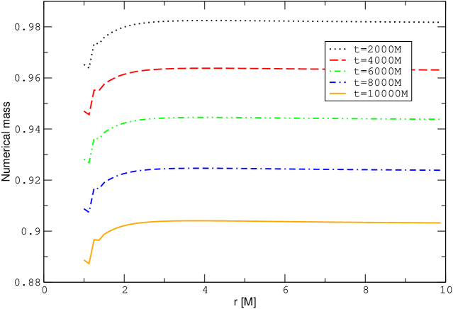
In figure 4 we plot ${\cal M}/M$ as a function of radius, for different times and $\Delta r=M/8$; the error is spread all over the domain and the mass decreases monotonically in time, which suggests that the black hole is moving through the grid (in the sense that $r\rightarrow r+t\times v_{num}$). We have verified that this is indeed the case (but, still, $v_{num}={\cal O}\left(\Delta r^{2}\right)$) by computing the (grid) location of the apparent horizon. For example, with $\Delta r=M/8$, after $10,000M$ the horizon has moved from $r_{h}=2M$ to $r_{h}=1.75M$, which accounts for the roughly ten percent error that the mass has at that time in figure 3:

$$\delta M\approx 1-r_{h}/(2M)\approx 0.1$$

We have tried different positions for both boundaries, with the inner one always inside the black hole and the outer one ranging from $10M$ to $1,000M$, and neither the stability nor the convergence of the simulations depended on such positions. In figures 5 and 6 we show the analogue of figures 2 and 3; with the outer boundary placed at $50M$, while still running the code up to $10^{3}$ crossing times (i.e. $t=50,000M$).

FIG. 5.: Same as for figure 2, but now with the outer boundary at $r=50M$.

FIG. 6.: Same as for figure 3, but now with the outer boundary at $r=50M$, as in the previous plot.

2 Gauge pulse falling into black hole

As discussed in Section III, the mode $u_{3}$ at the outer boundary is completely arbitrary. In this next test we let a gauge pulse enter the domain through the boundary. We thus use initial data corresponding to a Painlevé-Gullstrand slicing of a black hole of mass $M$, and fix $u_{3}$ at $r_{outer}$ by superposing, on top of the Painlevé-Gullstrand value, a Gaussian pulse described by

$$u_{3}(t)=u_{3}^{PG}\left(1+Ae^{-(t-t_{0})^{2}/\tilde{\sigma}^{2}}\right)\,.$$ (38)

FIG. 7.: The radial component of the metric, for a gauge pulse entering the domain through the outer boundary. The amplitude’s pulse grows as it approaches the inner boundary, falls into the black hole, and finally the metric settles down to a stationary one.

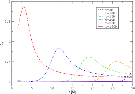
In figure 7 we present snapshots of the $g_{rr}$ component of the metric as a function of radius for different times. The width of the pulse is $\tilde{\sigma}=2M$, and it is centered at $t_{0}=5M$. The amplitude is quite large, $A=1$, corresponding to a $100\%$ “disturbance” of the stationary value. The resolution employed is $\Delta r=M/8$, and the domain extends from $r_{inner}=M$ to $r_{outer}=30M$. The pulse grows as it approaches the inner boundary (which is not surprising, since it happens even for a linear scalar equation propagating in a Schwarzschild background due to the effective non-trivial potential), $g_{rr}$ having a disturbance of more than $500\%$ that of the stationary value when it “crosses” the inner boundary. After the pulse falls into the black hole, the metric components gradually settle down to stationary values and the code runs for unlimited times.

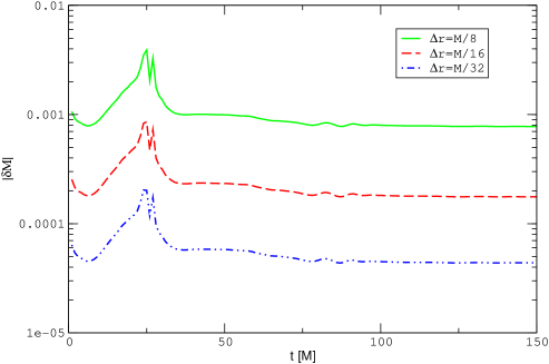
Since we are dealing with a vacuum spherically symmetric spacetime, the resulting spacetime must be a (dynamical) slicing of Schwarzschild. One way of corroborating this is to follow the Misner-Sharp mass. As can be seen in figure 8, where $|\delta M|$ is shown as a function of time for different resolutions, the numerical value of the mass does converge to this analytical prediction. Just as in the stationary case, the code runs for as long as wanted, and has a similar linear drift in the mass at late times. The growth in the errors around $t=30M$ seen in figure 8 are not due to the pulse entering the domain through the boundary (this happens at $t=5M$) but due to the pulse reaching the inner boundary, where all the gradients are steeper, and the huge growth in $g_{rr}$ is rather poorly resolved. Similar growths appear in the constraints (see figure 9), but they are still second-order convergent. It is indicative of the power of consistent boundary conditions that we can have such a big pulse entering the domain through the boundary, causing the spacetime to be so dynamical, that the code is stable and that the mass error is small (notice that even for a resolution as coarse as $\Delta r=M/8$ this error, while the pulse travels trough the domain, does not exceed one percent).

FIG. 8.: Mass error for a gauge pulse “falling” into the black hole. The peaks around $t=30M$ are caused by the pulse reaching the inner boundary. After the pulse falls into the black hole the spacetime settles to a stationary one, and at late times the mass has a linear drift, just as in the stationary evolutions.

FIG. 9.: $L_{2}$ norm of the Hamiltonian constraint for the same run shown in figure 8.

In equation (38) we wrote the boundary condition in that way (i.e. the Painlevé-Gullstrand value times a time dependent function) in order to have a measure of how large the pulse is compared to its stationary value. In the next simulations we will have a more physical idea of how strong these pulses can be in our code.

B Scalar field coupled to the black hole

As a last test of the approach we consider the case of a minimally coupled scalar field which also enters the computational domain through the outer boundary. As mentioned, only one scalar field mode is freely specifiable at the outer boundary. It is this mode which is chosen to describe an incoming pulse with amplitude $A$ and compact support in time as

$$u_{7}(t)=A(t-t_{I})^{4}(t-t_{F})^{4}\sin(\pi t)\,,$$

if $t\in[t_{I},t_{F}]$, and $u_{7}(t)=0$ otherwise. We choose $u_{3}=0$, and for the initial data we take that of a Painlevé-Gullstrand black hole of mass $M$. Note that one advantage of this is that one can perform non trivial simulations without solving the constraints initially, since one can provide, as we have done, a known solution of the constraints as initial data, and introduce the non trivial dynamics through the boundary (where all the treatment is algebraic), see also [20].

We have tried different amplitudes and time range for the pulse, obtaining stable discretizations in all cases. In order to illustrate the robustness of the approach we here show two examples. In the first one we show how the method can cope with considerably strong pulses (measured by the amount of energy that the black hole accretes), and in the second one the tails of the scalar field are computed and shown to agree with the expected result.

FIG. 10.: Change in the area of the apparent horizon, due to a quite narrow ($\Delta t=10M$) pulse of scalar field injected at the outer boundary, with a not very demanding resolution ($\Delta r=M/8$). The final mass of the black hole is more than twice the original one.

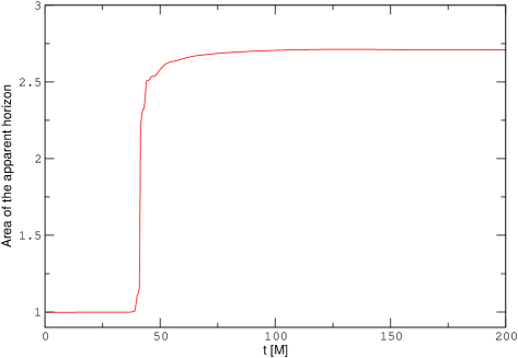
For the first case we chose $A=8$, $t_{I}=0,t_{F}=10M$, $\Delta r=M/10$ and the outer boundary at $r=50M$. Figure 10 illustrates the area of the apparent horizon as a function of time. Initially the area is $M$ and, as time progresses, it increases by $270\%$, until it reaches a stationary state describing, as expected, a Schwarzschild black hole of larger mass.

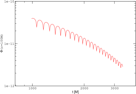
In the second case, in order to resolve the tails accurately, considerably finer resolution is needed. For this reason, we chose $\Delta r=M/50$ and place the outer boundary at $r=100M$. In order to measure the tails, we place four different observers: at $r=50,70,90$ and $100M$. The decay rate (of the form $\Phi\propto t^{-n}$) found by these observers is $n=-2.89,-2.97,-2.94$ and $-3.04$, respectively. These are in excellent agreement with the expected value of $n=-3$ [21]. Furthermore, the clean treatment of the outer boundary allows for accurate measurements even at the last point of the computational domain. Past works, which resorted to approximate boundary conditions, have observed that the boundary influenced the results when the observers were placed close to it.

FIG. 11.: Tail decay for the (time derivative of the) scalar field. The observer is located at the last grid point ($r=100M$) and measures a tail decay of $\Phi\propto t^{-3.04}$, in good agreement with the expected decay of $t^{-3}$. This is so mainly because of the clean treatment for the boundary.

Finally, we should mention that we have tried with different kinds of time dependent boundary conditions for the modes $u_{3}$ and $u_{7}$, and the results presented here do not depend on the particular choice made. Not only can we define pulses that last for a finite amount of time, as we have shown here, but we can define a time dependency that lasts forever (say, $u_{3}=A\sin(\omega t)$). In this sense, the large growth in the mass of the black hole mentioned above is what one can do with a pulse of width $10M$. In fact, one can increase arbitrarily the mass by using wider pulses, i.e. by slowly injecting scalar field energy through the boundary.

V Conclusions

In the present work we have presented additional support for the need to consider the constraint equations when defining boundary conditions. Although approximate boundary conditions (which are simpler to implement) can certainly be arranged to produce reliable simulations, for long term evolutions they have some important disadvantages:

• The inherent error introduced might accumulate, spoiling the physical outcome: For instance, even in the particular case of a binary black hole collision, the radiation is expected to be around $~{}5\%$ of the total mass of the system. Therefore, even small errors which accumulate over time can account for a significant percentage of the radiated energy. Since the outcome of some of these simulations will be used as templates for gravitational wave data analysis[22], one should minimize all possible waveform contaminating sources and diminish both amplitude and phase errors.

• Although the inherent error of approximate boundary conditions can be reduced by placing the outer boundary farther away from the sources, this amounts to having to compute the solution on a larger computational domain which naturally increases the cost of the simulation.

• Standard approximate boundary approaches pay little or no attention to the satisfaction of the constraints at the boundary. It is hard to conceive that they do not introduce constraint violating modes into the solution. Unless the implemented scheme is capable of damping these modes away, they will be present in the computational domain. A possible source of instabilities (though not necessarily the only one) in present implementations are, precisely, constraint violating modes, hence, it is important to eliminate all possible sources for these modes. It might happen that, in certain cases, the observed constraint violations are due to those particular implementations. Nevertheless, as the goal is to solve Einstein equations, sources of constraint violations must be removed. As mentioned, standard boundary treatments are likely to introduce these violations.

Furthermore, carefully designed boundary conditions are important in the case of artificial boundaries. These are boundaries which occur inside the computational domain where the computational mesh has regions with different resolutions (for instance in the case of adaptive mesh refinement) or has been subdivided into sub-domains which are treated independently (e.g. when using domain decomposition techniques). As these boundaries are purely artificial and introduced for convenience, it is imperative to count with a clean boundary treatment which eliminates (or at least minimizes) any spurious reflections or numerical noise.

Consequently, the search for accurate boundary conditions is of importance in present applications. The results presented in this work attest to that effect and suggest a practical and simple way to obtain such boundary conditions, which ensures constraint violating modes are absent by the very definition of the approach. Current work is devoted to applying the same techniques to 3D problems.

VI Acknowledgments

This work was supported by grants NSF-PHY-0090091, NSF-PHY-9800973, by Fundación Antorchas, and by the Eberly Family Research Fund at Penn State. It is a pleasure to thank O. Reula for discussions and helpful insights, and M. Choptuik, B. Kelly, L. Kidder, J. Pullin, R. Matzner, P. Laguna, M. Scheel, H. Shinkai, and S. Teukolsky for comments and suggestions. G.C. acknowledges E. Frymoyer for financial support, and L.L. acknowledges financial support from CITA (as a CITA National Fellow) and wishes to thank the University of South Africa (UNISA) for its hospitality where parts of this work were completed. Some computations were performed on the vn.physics.ubc.ca Beowulf cluster which was funded by the Canadian Foundation for Innovation (CFI). The Center for Gravitational Wave Physics is supported by the National Science Foundation under co-operative agreement PHY 01-14375.

A Evolution equations

The main variables propagate according to

$$\dot{g}_{rr} = \beta g_{rr}^{\prime}+2g_{rr}\beta^{\prime}-2\tilde{\alpha}g_{rr}^{1/2}g_{T}K_{rr}$$

$$\dot{g}_{T} = \beta g_{T}^{\prime}-2\tilde{\alpha}g_{rr}^{1/2}g_{T}K_{T}+\frac{2\beta g_{T}}{r}$$

$$\dot{K}_{rr} = \beta K_{rr}^{\prime}-\tilde{\alpha}g_{rr}^{-1/2}g_{T}f_{rrr}^{\prime}-\tilde{\alpha}^{{}^{\prime\prime}}g_{rr}^{1/2}g_{T}-6g_{T}^{-1}g_{rr}^{1/2}\tilde{\alpha}f_{rT}^{2}+4g_{T}r^{-1}g_{rr}^{1/2}\tilde{\alpha}^{\prime}-6g_{T}r^{-2}g_{rr}^{1/2}\tilde{\alpha}+2K_{rr}\beta^{\prime}-$$

$$2g_{T}g_{rr}^{1/2}\tilde{\alpha}\Phi^{2}-g_{T}g_{rr}^{-1/2}\tilde{\alpha}K_{rr}^{2}+2g_{rr}^{1/2}\tilde{\alpha}K_{rr}K_{T}-8g_{rr}^{-1/2}\tilde{\alpha}f_{rT}f_{rrr}+2g_{T}g_{rr}^{-3/2}\tilde{\alpha}f_{rrr}^{2}+$$

$$2g_{T}r^{-1}g_{rr}^{-1/2}\tilde{\alpha}f_{rrr}-g_{T}g_{rr}^{-1/2}\tilde{\alpha}^{\prime}f_{rrr}$$

$$\dot{K}_{T} = \beta K_{T}^{\prime}-\tilde{\alpha}g_{T}g_{rr}^{-1/2}f_{rT}^{\prime}+2\beta r^{-1}K_{T}+g_{T}r^{-2}g_{rr}^{1/2}\tilde{\alpha}+\tilde{\alpha}g_{T}K_{T}K_{rr}g_{rr}^{-1/2}-g_{T}f_{rT}\tilde{\alpha}^{\prime}g_{rr}^{-1/2}-2\tilde{\alpha}f_{rT}^{2}g_{rr}^{-1/2}$$

$$\dot{f}_{rrr} = \beta f_{rrr}^{\prime}-\tilde{\alpha}g_{rr}^{1/2}g_{T}K_{rr}^{\prime}-4g_{rr}^{3/2}\tilde{\alpha}^{\prime}K_{T}+12g_{T}^{-1}g_{rr}^{3/2}\tilde{\alpha}K_{T}f_{rT}-4g_{rr}^{1/2}\tilde{\alpha}K_{T}f_{rrr}-g_{T}g_{rr}^{-1/2}\tilde{\alpha}K_{rr}f_{rrr}-$$

$$10g_{rr}^{1/2}\tilde{\alpha}K_{rr}f_{rT}+3f_{rrr}\beta^{\prime}+g_{rr}\beta^{{}^{\prime\prime}}-\tilde{\alpha}^{\prime}g_{rr}^{1/2}g_{T}K_{rr}+2r^{-1}g_{T}g_{rr}^{1/2}\tilde{\alpha}K_{rr}+8r^{-1}g_{rr}^{3/2}\tilde{\alpha}K_{T}+4\tilde{\alpha}g_{rr}^{3/2}g_{T}\Phi\Pi$$

$$\dot{f}_{rT} = \beta f_{rT}^{\prime}-\tilde{\alpha}g_{rr}^{1/2}g_{T}K_{T}^{\prime}+\beta^{\prime}f_{rT}-\tilde{\alpha}^{\prime}g_{rr}^{1/2}g_{T}K_{T}+2g_{rr}^{1/2}\tilde{\alpha}K_{T}f_{rT}-\tilde{\alpha}g_{rr}^{-1/2}K_{T}f_{rrr}g_{T}+2r^{-1}\beta f_{rT}$$

$$\dot{\Phi} = \beta\Phi^{\prime}-\tilde{\alpha}g_{rr}^{1/2}g_{T}\Pi^{\prime}-g_{rr}^{-1/2}\tilde{\alpha}g_{T}\Pi f_{rrr}+2\tilde{\alpha}g_{rr}^{1/2}\Pi f_{rT}+2r^{-1}\tilde{\alpha}g_{rr}^{1/2}g_{T}\Pi-\tilde{\alpha}^{\prime}g_{rr}^{1/2}g_{T}\Pi+\Phi\beta^{\prime}$$

$$\dot{\Pi} = \beta\Pi^{\prime}-g_{rr}^{-1/2}\tilde{\alpha}g_{T}\Phi^{\prime}+g_{rr}^{-1/2}\tilde{\alpha}g_{T}\Pi K_{rr}+2\tilde{\alpha}g_{rr}^{1/2}\Pi K_{T}-4g_{rr}^{-1/2}\tilde{\alpha}\Phi f_{rT}+2r^{-1}g_{rr}^{-1/2}\tilde{\alpha}g_{T}\Phi-g_{rr}^{-1/2}g_{T}\Phi\tilde{\alpha}^{\prime}$$

B Excision of the singularity

The issue of excision is a non trivial one, even if dealing with a strongly hyperbolic formulation of Einstein’s equations, and even ignoring the constraints. The point is that, depending on the formulation, modes can leave the black hole. Even though these modes cannot be physical, they would need boundary conditions in any case in order to fix the solution. If one, for example, extrapolated all variables in such a situation, one would be implicitly be giving boundary conditions that depend on the discretization and that might not have a consistent limit as the grid spacing is decreased. Here we show a simple example to illustrate this point.

We start with a formulation widely used in numerical relativity, the ADM one (more precisely, the equations arising from $R_{ab}=0$), and we choose exact lapse and exact co-shift (that is, the covariant shift). We use the same notation as in the body of the paper, except that now $N=N(t,r)$ and $\beta_{r}=\beta_{r}(t,r)$ are prescribed as arbitrary functions of spacetime. In spherically symmetry, the evolution equations for such a formulation are

$$\dot{g}_{rr} = -\frac{\beta_{r}g_{rr}^{\prime}}{g_{rr}}+2\beta_{r}^{\prime}-2NK_{rr}$$ (B1)

$$\dot{g}_{T} = \frac{\ \beta_{r}g_{T}^{\prime}}{g_{rr}}+2\frac{\beta_{r}g_{T}}{rg_{rr}}-2NK_{T}$$ (B2)

$$\dot{K}_{rr} = -\frac{1}{2g_{rr}^{2}g_{T}^{2}r}\left(-2g_{T}^{2}r\beta_{r}K_{rr}^{\prime}g_{rr}-4g_{T}^{2}rK_{rr}\beta_{r}^{\prime}g_{rr}+4g_{T}^{2}rK_{rr}\beta_{r}g_{rr}^{\prime}+\right.$$ (B5)

$$2Ng_{rr}^{2}g_{T}^{{}^{\prime\prime}}rg_{T}+4Ng_{rr}^{2}g_{T}^{\prime}g_{T}-Ng_{rr}g_{rr}^{\prime}rg_{T}g_{T}^{\prime}-2Ng_{rr}g_{rr}^{\prime}g_{T}^{2}-Ng_{rr}^{2}(g_{T}^{\prime})^{2}r+$$

$$\left.2Ng_{rr}K_{rr}^{2}g_{T}^{2}r-4Ng_{rr}^{2}K_{rr}g_{T}rK_{T}+2N^{{}^{\prime\prime}}g_{rr}^{2}g_{T}^{2}r-g_{rr}^{\prime}N^{\prime}g_{rr}g_{T}^{2}r\right)$$

$$\dot{K}_{T} = \frac{1}{4r^{2}g_{rr}^{2}}\left(4\beta_{r}r^{2}g_{rr}K_{T}^{\prime}+8\beta_{r}rg_{rr}K_{T}-2Ng_{T}^{{}^{\prime\prime}}r^{2}g_{rr}-8Ng_{T}^{\prime}rg_{rr}+Ng_{rr}^{\prime}r^{2}g_{T}^{\prime}+2Ng_{rr}^{\prime}rg_{T}+\right.$$ (B7)

$$\left.4Ng_{rr}^{2}-4Ng_{rr}g_{T}+4NK_{T}r^{2}g_{rr}K_{rr}-2r^{2}N^{\prime}g_{rr}g_{T}^{\prime}-4rN^{\prime}g_{rr}g_{T}\right)$$

Note that in the previous equations, only $g_{T}$ appears with second derivatives. This means that we can rewrite this system as a first-order one by introducing just one new variable, $z:=g_{T}^{\prime}$; i.e. $\dot{u}=Au^{\prime}+B$, where $u=(g_{rr},g_{T},K_{rr},K_{T},z)^{\dagger}$.

As an evolution equation for $z$ we make the simplest possible choice: we just take the spatial derivative of the r.h.s. Eq. (B2) (i.e. we do not add the constraints to this new equation). Also, we replace everywhere $g_{T}^{\prime}$ by $z$. The principal part is, then:

$$A=\left(\begin{array}[]{ccccc}\displaystyle{-\frac{\beta_{r}}{g_{rr}}}&0&0&0&0\\ &&&&\\ 0&0&0&0&0\\ \displaystyle{\frac{-4rg_{T}K_{rr}\beta_{r}+2Ng_{rr}g_{T}+Nzrg_{rr}+rg_{rr}g_{T}N^{\prime}}{2rg_{rr}^{2}g_{T}}}&0&\displaystyle{\frac{\beta_{r}}{g_{rr}}}&0&\displaystyle{-\frac{N}{g_{T}}}\\ &&&&\\ \displaystyle{\frac{N(rz+2g_{T})}{4rg_{rr}^{2}}}&0&0&\displaystyle{\frac{\beta_{r}}{g_{rr}}}&\displaystyle{-\frac{N}{2g_{rr}}}\\ &&&&\\ \displaystyle{-\frac{\beta_{r}(rz+2g_{T})}{rg_{rr}^{2}}}&0&0&-2N&\displaystyle{\frac{\beta_{r}}{g_{rr}}}\end{array}\right)$$

This matrix has as eigenvalues and eigenvectors

$$u_{1}=\left[1,0,-\frac{g_{rr}N^{\prime}-4\beta_{r}K_{rr}}{4\beta_{r}g_{rr}},0,\frac{rz+2g_{T}}{2rg_{rr}}\right]\;\;\;,\left(v_{1}=-\frac{\beta_{r}}{g_{rr}}\right)$$ (B8)

$$u_{2}=\left[0,0,1,0,0\right]\;\;\;,\left(v_{2}=\frac{\beta_{r}}{g_{rr}}\right)$$ (B9)

$$u_{3}=\left[0,1,0,0,0\right]\;\;\;\left(v_{3}=0\right)$$ (B10)

$$u_{4}=\left[0,0,-\frac{g_{rr}^{1/2}}{g_{T}},-\frac{1}{2g_{rr}^{1/2}},1\right]\;\;\;,\left(v_{4}=\frac{\beta_{r}+Ng_{rr}^{1/2}}{g_{rr}}\right)$$ (B11)

$$u_{5}=\left[0,0,\frac{g_{rr}^{1/2}}{g_{T}},\frac{1}{2g_{rr}^{1/2}},1\right]\;\;\;,\left(v_{5}=\frac{\beta_{r}-Ng_{rr}^{1/2}}{g_{rr}}\right)$$ (B12)

The determinant of the matrix that diagonalizes $A$ is proportional to

$$\frac{(-4K_{rr}\beta_{r}+g_{rr}N^{\prime})(rz+2g_{T})^{2}}{64g_{rr}^{7/2}\beta_{r}r^{2}}\;,$$ (B13)

the system being strongly hyperbolic unless this determinant is zero. For the usual slicings of Schwarzschild (Painlevé-Gullstrand, Kerr-Schild, time harmonic and full harmonic slicings) expression (B13) is different from zero, so the system is, indeed, strongly hyperbolic, and the same will hold for (perhaps slight) distortions of those spacetimes. Now, it is known that one has to give initial data and boundary conditions to the incoming characteristic modes in order to fix the solution in such a system. The point is that here there is always a negative eigenvalue (whose corresponding eigenmode will thus propagate in the direction of increasing $r$, in particular, leaving the black hole): if $\beta_{r}\neq 0$, these eigenmode is either $u_{1}$ or $u_{2}$, while the mode is $u_{5}$ if $\beta_{r}=0$.

It is important to point out that whether modes leave or not the black hole strongly depends on the particular formulation that one is dealing with. For example, using exactly the same formulation (ADM in spherical symmetry) with other choices of lapse and shift (such that they ‘lock’ the area) also gives strongly hyperbolic formulations when rewritten in first order form, but they do not have modes leaving the domain (see [23]). Also, if one uses exact-lapse and exact-shift (as opposed to exact co-shift), the system is only weakly hyperbolic and, thus, the characteristic modes are not complete but, in any case, they do not leave the black hole (see, also, [23]). What we want to emphasize here is that superluminal modes can appear quite naturally, even in standard formulations.

REFERENCES

- [1] L. Lehner, Class. Quant. Grav. 18, R25 (2001).
- [2] M. W. Choptuik, Phys. Rev. D 44, 3124 (1991).
- [3] R. L. Marsa and M. W. Choptuik, Phys. Rev. D 54, 4929 (1996); E. P. Honda and M. W. Choptuik, hep-ph/0110065; M. Shibata and T. Nakamura, Phys. Rev. D 52, 5428 (1995); R. Gomez, in Proceedings of the Binary Black Hole Workshop, edited by R. Matzner (Los Alamos, NM, unpublished, 1997).
- [4] H. Friedrich and A. Rendall, in Einstein’s Field Equations and their Physical Implications, Lecture Notes in Physics, edited by B. G. Schmidt (Springer-Verlag, Berlin, 2000), pp. 127-223; O. Reula, Living Rev. Rel. 1, 3 (1998).
- [5] H. Friedrich and G. Nagy, Comm. Math. Phys. 204, 691 (1999).
- [6] J. Bardeen and L. Buchman, private communication (2001); B. Szilagyi, B, Schmidt, and J. Winicour, gr-qc/0106026; M. Iriondo and O. Reula, gr-qc/0102027 ; B. Szilagyi, R. Gomez, N. T. Bishop, and J. Winicour, Phys. Rev. D 62 104006 (2000); R. Matzner, in Colliding Black Holes: Mathematical Issues in Numerical Relativity, edited by D. Eardley (Santa Barbara, 2000, http://online.itp.ucsb.edu/online/numrel00/).
- [7] S. Frittelli, Phys. Rev. D 55, 5992 (1997).
- [8] G. Gook, Living Rev. Rel. 3, 5 (2000).
- [9] B. Gustaffson, H. Kreiss, and J. Oliger, Time Dependent Problems and Difference Methods (Wiley, New York, 1995).
- [10] G. Calabrese et. al, in preparation.
- [11] J. Thornburg, Class. and Quantum Grav. 14, 1119 (1987).
- [12] A. Anderson and J. W. York, Jr., Phys. Rev. Lett. 82, 4384 (1999).
- [13] S. Frittelli and O. A. Reula, J. Math. Phys. 40, 5143 (1999).
- [14] L. E. Kidder, M. A. Scheel, and S. A. Teukolsky, Phys. Rev. D 64, 064017 (2001).
- [15] L. E. Kidder, M. A. Scheel, S. A. Teukolsky, E. D. Carlson, and G. B. Cook, Phys. Rev. D 62, 084032 (2000).
- [16] E. Seidel and W. M. Suen, Phys. Rev. Lett 69 (1992); M. Alcubierre and B. Schutz, J. Comp. Phys. 112 (1994); C. Gundlach and P. Walker, Class. Quant. Grav. 16, 991 (1999); M. Scheel et al, Phys. Rev. D 56, 6320 (1997); L. Lehner, M. Huq, and D. Garrison, Phys. Rev. D 62, 084016 (2000).
- [17] H. Kreiss and J. Oliger, Methods for the approximate solution of time independent problems (GARP Publication Series, Geneva, 1973).
- [18] C. W. Misner, K. S. Thorne, and J. A. Wheeler, Gravitation (Freeman, New York, New York, 1973).
- [19] O. Sarbach and M. Tiglio, Phys. Rev. D 64, 084016 (2001).
- [20] M. Iriondo and O. Reula, to appear in Phys. Rev. D, gr-qc/0102027.
- [21] C. Gundlach, R. H. Price, and J. Pullin, Phys. Rev. D 49, 883 (1994); Phys. Rev. D 49, 890 (1994). E. Ching, P. Leung, W. M. Suen and K. Young, Phys. Rev. Lett. 74 (1995) 2414.
- [22] E. Flanagan and S. A. Hughes, Phys. Rev. D 57, 4566 (1998); Phys. Rev. D 57, 4535 (1998).
- [23] B. Kelly et. al., Phys. Rev. D 64, 084013 (2001).