The Gravitational Cherenkov Radiation

Abstract

An example of discontinuity of the energy-momentum tensor moving at superluminal velocity is discussed. It is shown that the gravitational Mach cone is formed. The power spectrum of the corresponding Cherenkov radiation is evaluated.

1 Introduction

According to current beliefs the traditional relativity theory excludes the possibility of superluminal motion. More detailed analysis shows that this constraint actually concerns either information exchange between various events in a space-time or motion of material bodies. It should be noted however that, strictly speaking, the concept of information is beyond physics as long as there is no physical definition (except purely tautological ones) of a material body. Hyperbolizing a bit one may say that relativity imposes no limitations on propagation velocity of physical quantities like charge, mass etc.

An everyday life example of a superluminal charge motion, which may be found in many physical laboratories, is an image of an electron beam at an oscilloscope screen. With an oscilloscope operating, say, at 1 GHz sweep frequency, the velocity of the charge spot would exceed the speed of light if the screen is more than 30 cm wide. Another example is a light spot scanning across a dielectric surface and producing, therefore, the superluminal polarization wave. Evidently, these are the examples of superluminal phase velocities and there are no contradictions with the conformist approach to causality. However, from the viewpoint of electrodynamics a charge spot behaves like a real superluminal charge and it may emit the Cherenkov radiation even in vacuum.

Seemingly, for the first time the Cherenkov radiation of a reflected light spot was discussed by Franck [1]. Later, a number of detailed theoretical studies was performed; see, e.g., the review papers [2, 3, 4]. The rumor runs that this radiation was experimentally observed; however, I failed to find the reference.

It was pointed out (e.g.,[2]) that similar gravitational radiation may be emitted by a gravitational wave spot or a superluminal mass spot. However, to my knowledge, there was no detailed study of the emitted gravitational wake. In the present note the linearized Einstein equations are used to investigate the structure of gravitational field behind a superluminal mass spot.

2 Model

A model discussed in this paper is depicted in Fig. 1. Imagine two infinitesimally thin massive threads moving at an angle towards the x-axis. The threads collide at a certain point and form a new composite thread due to some inelastic process, e.g., a chemical reaction. At an instant of collision every atom experiences infinite deceleration that, presumably, should give rise to the gravitational bremsstrahlung.

Let’s choose the reference frame so that the velocities of the threads are $\boldsymbol{\beta}=\beta\boldsymbol{n}=\beta(\cos\theta,\sin\theta,0)$ and $\boldsymbol{\beta}^{\prime}=\beta\boldsymbol{n}^{\prime}=\beta(\cos\theta,-\sin\theta,0)$. The mass densities of both threads are equal and in the chosen frame the net density prior to the collision is given by $j^{0}(\xi)=\sigma\delta(z)[\delta(\boldsymbol{n}\cdot\boldsymbol{r}-\beta t)+\delta(\boldsymbol{n}^{\prime}\cdot\boldsymbol{r}-\beta t)]$, where $\sigma$ is the mass per unit length and $\xi=(t,x,y,z)=(t,\boldsymbol{r})$. It is assumed that $0<\theta<\pi/2$ and the speed of light is unity. The flat space-time metric is used, $ds^{2}=\eta_{\mu\nu}d\xi^{\mu}d\xi^{\nu}=-dt^{2}+d\boldsymbol{r}^{2}$.

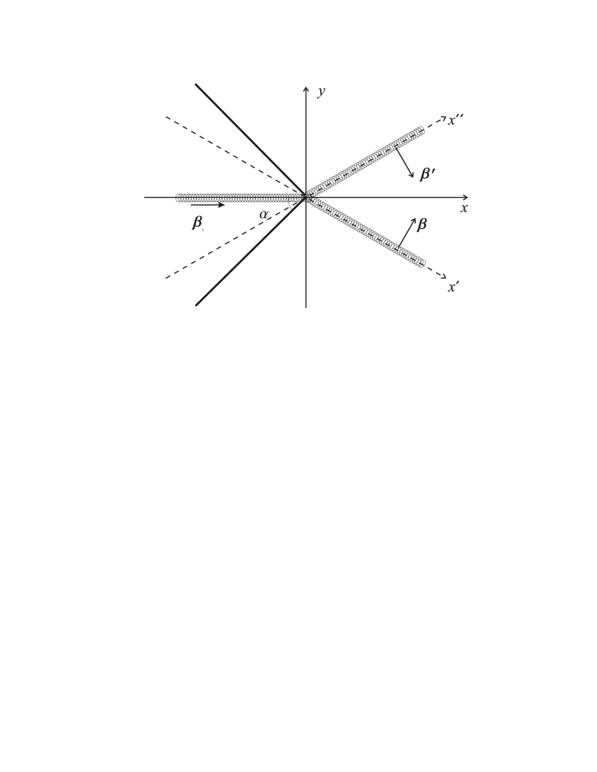
Figure 1: Two colliding massive threads depicted as spirals produce the gravitational radiation at the Mach cone (heavy line).

Let $x_{0}(t)$ be the coordinate of the intersection point; evidently, $x_{0}(t)=\beta t/\cos\theta\equiv ut$. Depending on the angle of incidence, $\theta$, the velocity, $u$, of the intersection point may be either subluminal or superluminal.

Let the threads be composed of a zero-pressure ideal gas. Therefore, the energy-momentum tensor prior to the collision is written as

$$T^{(+)\mu\nu}(\xi)=\sigma\delta(z)\left[\delta(\boldsymbol{n}\cdot\boldsymbol{r}-\beta t)\tau^{\mu\nu}(\boldsymbol{\beta})+\delta(\boldsymbol{n}^{\prime}\cdot\boldsymbol{r}-\beta t)\tau^{\mu\nu}(\boldsymbol{\beta}^{\prime})\right],$$ (1)

where

$$\tau^{00}(\beta)=\gamma(\beta),\qquad\tau^{0i}(\beta)=\gamma(\beta)\beta^{i},\qquad\tau^{ij}(\beta)=\gamma(\beta)\beta^{i}\beta^{j},$$

and $\gamma(\beta)=1/\sqrt{1-\beta^{2}}$.

Due to the symmetry of the problem the composite thread formed after the collision is situated at the x-axis and its energy-momentum tensor may be written as

$$T^{(-)\mu\nu}(\xi)=\sigma_{1}\delta(z)\delta(y)\tau^{\mu\nu}(\boldsymbol{\beta}_{1}).$$ (2)

Integrating (1,2) over the appropriate two-dimensional surfaces we find that the requirement of energy-momentum conservation results in

$$\boldsymbol{\beta}_{1}=(\beta\cos\theta,0,0),\qquad\sigma_{1}=\frac{2\sigma\gamma(\beta)}{\sin\theta\gamma(\beta_{1})},$$ (3)

that is, the x-component of the thread velocity remains unchanged. It should be pointed out that we expect that a part of the kinetic energy of the colliding threads is carried away by the gravitational bremsstrahlung. However, in the linear approximation, which we are going to implement, the influence of radiation losses on the motion and the mass of the composite thread is evidently negligible.

Thus, the net energy-momentum tensor is

$$T^{\mu\nu}(\xi)=T^{(+)\mu\nu}(\xi)\vartheta(x-ut)+T^{(-)\mu\nu}(\xi)\vartheta(ut-x),$$ (4)

where $\vartheta(x)$ is the Heaviside’s step function.

It should also be noted that although this model provides conservation of energy and momentum, $T^{\mu\nu}_{\ \ ,\,\nu}=0$, the mass is a non-conserving quantity: $\sigma_{1}>2\sigma$ in Eq. (3). This is the evident consequence of including non-gravitational interactions (e.g., chemical reactions) into the model that results in the mass defect. On the other hand, we can easily think out various models with mass conservation and energy losses. This may be, for example, a single massive thread moving at an angle towards an immobile absolutely rigid adhesive screen. The most essential feature of these models is the discontinuity of the energy-momentum moving at superluminal phase velocity. The problem is what kind of gravitational field is produced by the discontinuity.

3 Mach cone

Our goal here is to analyze the solution of the linearized Einstein equations with the energy-momentum tensor given by Eq. (4). Keeping the notation of [5] the d’Alembert equation for the distortion of the metric tensor is

$$-\bar{h}^{\mu\nu}_{\ \ ,}{}^{\ \lambda}_{\lambda}=16\pi T^{\mu\nu},$$ (5)

where

$$g^{\mu\nu}=\eta^{\mu\nu}+h^{\mu\nu}\equiv\eta^{\mu\nu}+\bar{h}^{\mu\nu}-\frac{1}{2}\eta^{\mu\nu}\bar{h}^{\lambda}_{\ \lambda}.$$ (6)

Since the energy-momentum tensor (4) is composed of three parts, the solution of Eq. (5) is also a superposition of three retarded solutions. First, consider the solution of the d’Alembert equation conditioned by the composite thread at $x<ut$. Let $f^{(-)}(\xi)$ be the retarded solution of the equation

$$\square f^{(-)}(\xi)=4\pi\vartheta(ut-x)\delta(y)\delta(z)$$ (7)

that explicitly is written as

$$f^{(-)}(\xi)=\int\limits^{\infty}_{-\infty}\frac{ds}{\sqrt{s^{2}+\rho^{2}}}\vartheta\left(-s-u\sqrt{s^{2}+\rho^{2}}+u\tau\right),$$ (8)

where $\tau=t-x/u$ and $\rho=\sqrt{y^{2}+z^{2}}$. The integral in Eq. (8) essentially depends on the velocity of the tip of the thread, $u$. In what follows we focus on the most interesting superluminal motion. If $u>1$ then

$$f^{(-)}(\xi)=2\vartheta(\tau-\cos\alpha\rho)\cosh^{-1}\left(\frac{\tau}{\cos\alpha\rho}\right),$$ (9)

where $\sin\alpha=1/u$, i.e. the result is non-zero inside the Mach cone

$$\tau\geq\cos\alpha\rho$$ (10)

depicted by the heavy line in Fig. 1.

In order to evaluate the field produced by the colliding threads at $x>ut$ note that

$$\vartheta(x-ut)\delta(\boldsymbol{n}\cdot\boldsymbol{r}-\beta t)=\gamma(\beta)\delta(y^{\prime})\vartheta(x^{\prime}-u^{\prime}t^{\prime}),$$

where $t^{\prime},x^{\prime},y^{\prime},z^{\prime}$ are own frame coordinates of the moving thread. The corresponding Lorentz transform is composed of a boost and a rotation around the $z$ axis:

$$t^{\prime} = \gamma(t-\beta\boldsymbol{n}\cdot\boldsymbol{r})$$

$$x^{\prime} = x\sin\theta-y\cos\theta$$

$$y^{\prime} = \gamma(-\beta t+\boldsymbol{n}\cdot\boldsymbol{r})$$ (11)

$$z^{\prime} = z$$

The speed of the tip of the moving part of the thread in its own frame is $u^{\prime}=\beta\gamma\tan\theta$; evidently, if $u>1$ then $u^{\prime}>1$ and vice versa.

The solution of the d’Alembert equation

$$\square f^{(+)}(\xi)=4\pi\vartheta(x-ut)\delta(\boldsymbol{n}\cdot\boldsymbol{r}-\beta t)\delta(z)$$ (12)

is given by

$$f^{(+)}(\xi) = \gamma(\beta)\int\limits^{\infty}_{-\infty}\frac{ds}{\sqrt{s^{2}+\rho^{\prime 2}}}\vartheta\left(s+u^{\prime}\sqrt{s^{2}+\rho^{\prime 2}}-u\tau^{\prime}\right)$$ (13)

$$= \gamma(\beta)\left[-2\ln\rho^{\prime}-2\vartheta(\tau^{\prime}-\cos\alpha^{\prime}\rho^{\prime})\cosh^{-1}\left(\frac{\tau^{\prime}}{\cos\alpha^{\prime}\rho^{\prime}}\right)\right],$$ (14)

where $\tau^{\prime}=t^{\prime}-x^{\prime}/u^{\prime}$, $\rho^{\prime}=\sqrt{y^{\prime 2}+z^{2}}$ and $\sin\alpha^{\prime}=1/u^{\prime}$. One can easily verify that inequalities $\tau^{\prime}\geq\cos\alpha^{\prime}\rho^{\prime}$ and (10) defines the same conical area in space.

Comparing Eqs. (8,13), we see that due to the different signs of the arguments of the $\vartheta$-functions the integral (13) is a composition of the logarithmic potential produced by the infinitely thin massive thread and the wake wave analogous to the one excited by the composite part (9). However unlike Eq. (9), the structure of the wake field (14) is not axially-symmetric in the initial reference frame. It should also be noted that there is no logarithmic singularity at $x^{\prime}<0$ in Eq. (14), i.e. at the left side of the $x^{\prime}$-axis shown by the dashed line in Fig. 1, which is always inside the Mach cone.

The field of the second thread is evaluated in the same way. Finally, the resulting metric perturbation is given by

$$\bar{h}^{\mu\nu}(\xi) = -8\sigma\gamma(\beta)\left\{\tau^{\mu\nu}(\boldsymbol{\beta})\left[\ln\rho^{\prime}+\vartheta(\tau-\cos\alpha\rho)\cosh^{-1}\left(\frac{\tau^{\prime}}{\cos\alpha^{\prime}\rho^{\prime}}\right)\right]\right.$$ (15)

$$+ \left.\tau^{\mu\nu}(\boldsymbol{\beta}^{\prime})\left[\ln\rho^{\prime\prime}+\vartheta(\tau-\cos\alpha\rho)\cosh^{-1}\left(\frac{\tau^{\prime\prime}}{\cos\alpha^{\prime}\rho^{\prime\prime}}\right)\right]\right\}$$

$$+ \frac{16\sigma\gamma(\beta)}{\sin\theta\,\gamma(\beta_{1})}\tau^{\mu\nu}(\boldsymbol{\beta}_{1})\vartheta(\tau-\cos\alpha\rho)\cosh^{-1}\left(\frac{\tau}{\cos\alpha\rho}\right),$$

where the double primed variables are given by Eqs. (11) with $\theta$ replaced by $-\theta$.

Although Eq. (15) looks pretty bulky its structure is transparent. The field ahead of the collision point, $x>ut$ is a superposition of two logarithmic potentials distorted by the Lorentz transform. The field inside the Mach cone (10) also looks like the static one near the $x$-axis. However, the metric and some of the components of the Riemann tensor are divergent at the Mach cone. This is the evident consequence of the accepted model: taking into account the finite size of the threads would smooth this singularity.

4 Radiation field

The discussed collision process produce the Mach cone at the space-time fabric. However, it is obtained in the near zone and it is unclear whether there is any radiation field. The straightforward evaluation of the gravitational energy-momentum flux using Eq. (15) yields very complicated integrals. We can circumvent this difficulty implementing the procedure similar to the one used in electrodynamics [2, 3].

Suppose that the system as a whole is of large but finite size, $L$. Performing the time Fourier transform of Eq. (5) the asymptotic of $\bar{h}^{\mu\nu}(\omega,\boldsymbol{r})$ is written as ( e.g., [6])

$$\left.\bar{h}^{\mu\nu}(\omega,\boldsymbol{r})\right|_{r\gg L}=\frac{e^{i\omega r}}{r}\bar{\Lambda}^{\mu\nu}(\omega,\boldsymbol{s}),$$ (16)

where $\boldsymbol{s}=\boldsymbol{r}/r$ is the direction of the wave propagation and $\Lambda^{\mu\nu}(\omega,\boldsymbol{s})$ is the Fourier transform of the energy-momentum tensor (4),

$$\bar{\Lambda}^{\mu\nu}(\omega,\boldsymbol{s})=4\int dt\,d\boldsymbol{r}\,e^{i\omega t-i\omega\boldsymbol{sr}}\,T^{\mu\nu}(t,\boldsymbol{r})$$

$$= \frac{8\pi i\sigma}{\omega^{2}}\delta(s_{x}-1/u)\left\{\frac{\tau^{\mu\nu}(\boldsymbol{\beta})}{s_{y}-\sin\theta}+\frac{\tau^{\mu\nu}(\boldsymbol{\beta}^{\prime})}{s_{y}+\sin\theta}+\frac{2\gamma(\beta)}{\sin\theta\,\gamma(\beta_{1})}\tau^{\mu\nu}(\boldsymbol{\beta}_{1})\right\}.$$

Extracting the transverse traceless part of the metric perturbation, $h^{\mu\nu}$ (6), we obtain its spatial components

$$h^{TT}_{ij}=\frac{e^{i\omega t}}{r}\frac{8\pi i\sigma}{\omega^{2}}\delta(s_{x}-1/u)Q_{ij},$$ (18)

where

$$Q_{ij}=\frac{P_{ij}(\boldsymbol{\beta})}{s_{y}-\sin\theta}+\frac{P_{ij}(\boldsymbol{\beta}^{\prime})}{s_{y}+\sin\theta}+\frac{2\gamma(\beta)}{\sin\theta\,\gamma(\beta_{1})}P_{ij}(\boldsymbol{\beta}_{1})$$ (19)

and

$$P_{ij}(\boldsymbol{\beta})=\frac{1}{2}\left(\delta_{ij}-s_{i}s_{j}\right)+\gamma(\beta)(\beta_{i}-s_{i})(\beta_{j}-s_{j}).$$ (20)

Since the energy-momentum of the gravitational waves is $T^{GW}_{\mu\nu}=\langle h^{TT}_{ij,\mu}h^{TT}_{ij,\nu}\rangle/32\pi$, evaluating its $tr$-component and integrating over a sufficiently large sphere we get the power spectrum of the emitted radiation

$$\frac{dW_{\omega}(\chi,\psi)}{dt}=\frac{2u\sigma^{2}}{\omega}\delta(\cos\chi-1/u)Q_{ij}Q_{ij}\sin\chi d\chi\,d\psi\,d\omega,$$ (21)

where $\chi,\psi$ are spherical angles corresponding to the direction of the wave propagation, $\boldsymbol{s}=(\cos\chi,\;\sin\chi\,\cos\psi,\;\sin\chi\,\sin\psi)$.

The power spectrum (21) is of typical Cherenkov character. The $\delta$-function indicates that the waves obeying the resonance condition $\omega=k_{x}u$ only are emitted. The complicated angular dependence hidden in $Q_{ij}^{2}$ is specific for the accepted model.

Due to the $1/\omega$ dependence in Eq.(21) the net emitted power diverges. (The same problem also arises in electrodynamics.) The effective cut-off may be provided by finite length of the threads that makes integrals convergent in the low-frequency band. The high-frequency cut-off arises due to the finiteness of the deceleration in the process collision and/or due to the finite diameter of the threads.

5 Conclusion

We have shown that a superluminal discontinuity of the energy-momentum tensor results in the formation of the gravitational Mach cone and the corresponding gravitational Cherenkov radiation. Although we took special care of the energy conservation, the problem is not self-consistent: a part of the energy and momentum is carried away by gravitational radiation. This would result in a reaction force acting upon the emitting system.

References

- [1] Franck IM Izv. Akad. Nauk SSSR Ser. Fiz. 63 (1942)
- [2] Bolotovskii BM, and Ginzburg VL Usp. Fiz. Nauk 106 577 (1972) [Sov.Phys. Usp. 15 184 (1972)]
- [3] Ginzburg VL, Teoreticheskaya Fizika i Astrofizika (Theoretical Physics and Astrophysics) (Moscow: Nauka, 1981) [Translated into English (Oxford, New York: Pergamon Press, 1979)]
- [4] Barsukov KA, and Popov VN, Usp. Fiz. Nauk 166 1245 (1996)[Physics Uspekhi 39 1181 (1996)]
- [5] Misner CW, Thorne KS, and Wheeler JA, Gravitation (Freeman, San Francisco, 1973, Chapter 18).
- [6] L.D. Landau and E.M. Lifshitz, The Classical Theory of Field (Pergamon, Oxford, 1975, Chapter 9).