Second post-Newtonian gravitational wave polarizations for compact binaries in elliptical orbits

A. Gopakumar1,2 and Bala R. Iyer 3 1Department of Physics and McDonnell Center for the Space Sciences,
Washington University, St. Louis, MO 63130, U.S.A
2Physical Research Laboratory, Navrangpura, Ahmedabad 380 009, India
3Raman Research Institute, C.V. Raman Avenue, Sadashivanagar, Bangalore 560080, India
Abstract

The second post-Newtonian (2PN) contribution to the ‘plus’ and ‘cross’ gravitational wave polarizations associated with gravitational radiation from non-spinning, compact binaries moving in elliptic orbits is computed. The computation starts from our earlier results on 2PN generation, crucially employs the 2PN accurate generalized quasi-Keplerian parametrization of elliptic orbits by Damour, Schäfer and Wex and provides 2PN accurate expressions modulo the tail terms for gravitational wave polarizations incorporating effects of eccentricity and periastron precession.

pacs:
PACS numbers: 04.25.Nx, 04.30.-w, 97.60.Jd, 97.60.Lf

I Introduction

Inspiralling compact binaries containing black holes and neutron stars are one of the most promising sources of gravitational radiation for both, almost operational ground based laser interferometric gravitational wave detectors like LIGO, VIRGO, GEO600 and TAMA300 [1] and the proposed space-based interferometer LISA [2]. To obtain an acceptable signal to noise ratio for detection in the terrestrial detectors, one needs to know a priori the binary’s orbital evolution in the inspiral waveform [3] at least upto third post-Newtonian order beyond the (Newtonian) quadrupole radiation. However, for the measurement of distance and position of the binary, it may be sufficient to know the two independent gravitational wave polarizations $h_{+}$ and $h_{\times}$ to only 2PN accuracy [4]. Perturbative computation via post-Newtonian (PN) expansions of the binary orbit and gravitational wave (GW) phase are complete to order $v^{5}$ beyond the standard quadrupole formula. Extension of the PN perturbative calculations by another two orders, to order $v^{7}$, is still not complete, because currently used PN techniques [5] leave undetermined a physically crucial parameter entering at the $v^{6}$ level in the gravitational wave flux [6]. More recently [7], it has been shown that by employing several re-summation techniques – to improve the convergence of the PN series – one could make optimal use of existing 2PN results to compute GW phasing. Resummed versions of 2PN accurate search templates may be just sufficient both for the detection and estimation of parameters of gravitational waves from inspiralling compact binaries of arbitrary mass ratio moving in quasi-circular orbits. For inspiralling non-spinning compact binaries of arbitrary mass ratio in quasi-circular orbits, both the 2PN accurate gravitational wave polarizations [8] and the associated orbital evolution have been explicitly computed [9, 10, 11]. A 2.5PN accurate formula for the orbital phase as a function of time has also been obtained [12]. These expressions are employed by various data analysis packages like LAL [13] to search for gravitational waves from inspiralling compact binaries.

The purpose of the present work is to obtain the ‘instantaneous’*** Following [10], we term contributions to the GW waveform which depends only on the state of the binary at the retarded instant as its ‘instantaneous’ part. 2PN contributions to the two gravitational wave polarizations for compact binaries moving in elliptical orbits. On the one hand, these expressions for $h_{+}$ and $h_{\times}$ represent gravitational waves from a binary evolving negligibly under gravitational radiation reaction, incorporating precisely upto 2PN order the effects of eccentricity and periastron precession, during that stage of inspiral when the orbital parameters are essentially constant over a few orbital revolutions. On the other hand, it is the first (and the necessary) step in the direction of obtaining ‘ready to use’ theoretical templates to search for gravitational waves from inspiralling compact binaries moving in quasi-elliptical orbits. The effect of radiation reaction on orbital evolution and its consequence on these gravitational waveforms for compact binaries in quasi-elliptical orbits is under investigation and will be discussed in the future [14].

Galactic binaries, in general, will be in circular orbits by the time they reach the final stage of inspiral. However, there exist astrophysical scenarios where compact binaries will have non-negligible eccentricity during the final inspiral phase. We will next review various such scenarios, some of them speculative, relevant for both ground and space based gravitational wave detectors.

Let us first consider cases that should be important for ground based interferometers. Intermediate mass black hole binaries – with total masses in the range $50\,M_{\odot}\leq M\leq$ (a few) $\times 10^{2}M_{\odot}$ – may well be the first sources to be detected by LIGO and VIRGO [15, 16]. Many recent astronomical observations, involving massive black hole candidates point to scenarios involving such compact binaries in eccentric orbits. The discovery of numerous bright compact X-ray sources with luminosities $L>10^{39}\,{erg/s}$ in several starburst galaxies and rapid time variation of their X-ray fluxes implies massive black holes as their central engines. It is suggested that these observations may be explained by the merger of globular clusters, containing black holes with $M>10^{3}\,M_{\odot}$, with its host galaxy [17]. However, $10^{3}\,M_{\odot}$ black hole present in the center of the globular cluster will have to be created by many coalescences of a $\geq 50\,M_{\odot}$ black hole with lighter ones and these binaries, in highly eccentric orbits, should be visible to ground based interferometers. This scenario may be contrasted with the one suggested in [18] which also involves compact binaries with high eccentricities. However, in this case, black hole binaries, weighing a few solar masses and residing in star clusters, get ejected from the cluster by superelastic encounter with other cluster members. These escaping binaries will have short periods and high eccentricities before merging. It is worth mentioning that numerical simulations dealing with supermassive blackhole formation, performed in the eighties, from a dense cluster of compact stars also indicate creation of short period intermediate mass black hole binaries in highly eccentric orbits [19].

Recently, there has been studies suggesting that spinning compact binaries may become chaotic [20]. The analysis involves numerical evolution of two spinning point masses using 2PN accurate equations of motion. The interesting result, observed only for a very restricted portion of the parameter space, is that the outcome of the evolution is highly sensitive to initial conditions. It is also observed that binaries whose initial orbits are circular may later become highly eccentric. These preliminary results present yet another scenario where eccentricity may become important.

Many of the potential sources for LISA [2] will be binaries in ‘quasi-elliptical’ orbits. We list them below, details and references to original papers may be found in [21]. First, LISA will be sensitive to massive black hole (MBH) coalescence involving $10^{3}$ to $10^{7}M_{\odot}$ black holes, upto 3 Gpc and beyond. It is likely that these binaries will be in eccentric orbits during inspiral, as they will be interacting with dense stellar clusters in the galactic nuclei where they usually reside. The second candidate involves compact objects orbiting MBH, where compact objects could be scattered into very short period eccentric orbits via gravitational deflections by other stars. Finally, LISA will be sensitive to thousands of binaries in our galaxy and many of these short period binaries will also be in ‘quasi-eccentric’ orbits. Interestingly, LISA will be highly sensitive to black hole binaries containing primordial black holes of mass $\sim 0.5\,M_{\odot}$. These binaries are one of the speculative candidates for MAssive Compact Halo Objects (MACHOs) [22]. It is also shown that [23, 24] the low frequency gravitational waves from black hole MACHO binaries in highly eccentric orbits would form a strong stochastic background in the frequency range $10^{-5}\,{\rm Hz}<f<10^{-1}\,{\rm Hz}$, where LISA will be most sensitive.

Finally, we observe that eccentricity will be an important parameter while searching for continuous gravitational wave sources in binary systems. Recently, it was shown that searching for gravitational waves from such systems, whose locations are exactly known, is computationally feasible [25]. For many such astrophysically interesting systems, we note that a post-Newtonian orbital description for generic orbits will be required.

The computation of the gravitational wave polarizations $h_{+}$ and $h_{\times}$ in terms of the orbital phase and frequency of the binary was discussed by Lincoln and Will [26], using the method of osculating orbital elements from celestial mechanics and the 2.5PN accurate Damour-Deruelle equations of motion [27, 28]. They studied the evolution of general orbits and obtained 1PN accurate expressions for $h_{+}$ and $h_{\times}$ for quasi-circular orbits. Later Moreno-Garrido, Mediavilla and Buitrago obtained polarization waveforms for binaries in elliptical orbits at Newtonian order with and without radiation reaction, studied the effects of orbital parameters and precession on gravitational wave amplitude spectrum and implications for data analysis [29, 30]. Analytic expressions for gravitational wave polarizations and far-zone fluxes, for elliptic binaries were obtained to 1.5PN order by Junker and Schäfer, and Blanchet and Schäfer [31, 32]. The 2PN accurate gravitational wave polarizations for inspiralling compact binaries moving in quasi-circular orbits was given by Blanchet, Iyer, Will and Wiseman [8]. For the above calculation they employed the 2PN accurate expressions for $h^{TT}_{ij}$, the transverse traceless part of the radiation field representing the deviation of the metric from the flat spacetime and $\left({d{\cal E}\over dt}\right)$, the far-zone energy flux obtained independently using two different formalisms [33, 9, 10, 11]. In the limiting case of a test particle orbiting a Schwarzschild black hole, perturbative calculations are extended to very high PN order. For example, in the case of very small mass ratios, polarization waveforms are obtained to 4PN order [34]. For the case of spinning compact objects in circular orbits, precessional, non-precessional and dissipative effects on the gravitational waveform due to spin-orbit and spin-spin interactions were studied extensively [35, 36, 37, 38]. We note that using the framework we employ here it may be possible to extend results of these papers to compact binaries of arbitrary mass ratio moving in elliptical orbits.

The basic aim of this paper is to obtain the instantaneous 2PN corrections to the ‘plus’ and ‘cross’ polarization waveforms for compact binaries of arbitrary mass ratio moving in elliptical orbits starting from the corresponding 2PN contributions to $h^{TT}_{ij}$ [11, 39]. As emphasized in [7], the gravitational wave observations of inspiralling compact binaries, is analogous to the high precision radio-wave observations of binary pulsars. The latter makes use of an accurate relativistic ‘timing formula’ based on the solution - in quasi-Keplerian parametrization - to the relativistic equation of motion for a compact binary moving in an elliptical orbit[40]. In a similar manner, the former demands accurate ‘phasing’, i.e. an accurate mathematical modeling of the continuous time evolution of the gravitational waveform. This requires for elliptical binaries, a convenient solution to the 2PN accurate equations of motion. A very elegant 2PN accurate generalized quasi-Keplerian parametrization for elliptical orbits has been implemented by Damour, Schäfer, and Wex [41, 42, 43, 44]. This representation is thus the most natural and best suited for our purpose to parametrize the dynamical variables that enter the gravitational waveforms. The complete 2PN accurate expressions for $h_{+}$ and $h_{\times}$ consists of the ‘instantaneous’ contribution computed here supplemented by tail contributions at 1.5PN and 2PN orders. The tail computations are not considered here; they must be computed and included in the future.

The paper is organized as follows: In section II, we present the details of the computation to obtain ‘instantaneous’ 2PN corrections to $h_{+}$ and $h_{\times}$ for inspiralling compact binaries moving in elliptical orbits. Section III deals with the influence of the orbital parameters on the waveform. Section IV comprises our concluding remarks.

II The 2PN gravitational wave polarization states

To compute the two independent gravitational wave polarization states $h_{+}$ and $h_{\times}$, one needs to choose a convention for the direction and orientation of the orbit. We follow the standard convention of choosing a triad of unit vectors composed of ${\bf N}$, a unit vector along the radial direction to the observer, p, a unit vector along the line of nodes, which coincides with y-axis and q, defined by ${\bf q}={\bf N}\times{\bf p}$ (see Fig. 1). The angle between N and the Newtonian angular momentum vector which lies along z-axis defines the inclination angle $i$ of the orbit. The orbital phase $\phi$ is measured from the positive x-axis in a counter clockwise sense, restricting the values of $i$ from 00 to ${1\over 2}\,\pi$. The two basic polarization states $h_{+}$ and $h_{\times}$ are given by

$\displaystyle h_{+}$ $\displaystyle=$ $\displaystyle{1\over 2}\biggl{(}p_{i}\,p_{j}-q_{i}\,q_{j}\biggr{)}\,h_{ij}^{TT}\,,$ (2)
$\displaystyle h_{\times}$ $\displaystyle=$ $\displaystyle{1\over 2}\biggl{(}p_{i}\,q_{j}+p_{j}\,q_{i}\biggr{)}\,h_{ij}^{TT}\,,$ (3)

where $h_{ij}^{TT}$ is the transverse-traceless (TT) part of the radiation field representing the deviation of the metric from the flat spacetime.

From Eqs. (II) it is clear that the explicit computation of 2PN corrections to $h_{+}$ and $h_{\times}$ requires the following: (a) The 2PN corrections to $h_{ij}^{TT}$, generally given in terms of the dynamical variables of the binary, namely $\,v^{2},{G\,m\over r},\dot{r},n_{i},v_{i},{\bf N.n},{\bf N.v}$, where r and v are respectively, the relative position and velocity vectors for the two masses $m_{1}$ and $m_{2}$ in the center of mass frame, $r=|{\bf r}|,v=|{\bf v}|,{\bf n}={{\bf r}\over r},\dot{r}={dr\over dt}$ and $m=m_{1}+m_{2}$. The unit vector N lies along the radial direction to the detector and is given by ${\bf N}={{\bf R}\over R}$, $R$ being the radial distance to the binary; and (b) A 2PN accurate orbital representation for elliptical orbits to parametrize these dynamical variables.

Before explaining in detail the procedure to compute 2PN contributions to $h_{+}$ and $h_{\times}$, we will first illustrate that computation by presenting in detail the Newtonian computations for $h_{+}$ and $h_{\times}$.

A The Newtonian GW Polarizations

At the leading Newtonian order, we have

$$(h^{TT}_{km})_{N}={4\,G\,\mu\,\over c^{4}\,R}{\cal P}_{ijkm}({\bf N})\biggl{(}v_{ij}-{G\,m\over r}\,n_{ij}\biggr{)}\,,$$ (4)

where ${\cal P}_{ijkm}({\bf N})$ is the usual transverse traceless projection operator projecting normal to N, $v_{ij}=v_{i}v_{j}\;,$ $\;n_{ij}=n_{i}n_{j}$; and $\mu$ is the reduced mass of the binary, given by $m_{1}\,m_{2}/m$. Note that the above contribution arises from the mass quadrupole moment of the binary.

There is no need to apply the TT projection in Eq. (4), and Eq. (II) at the leading order gives

$\displaystyle h_{+}$ $\displaystyle=$ $\displaystyle{2\,G\,\mu\over c^{4}\,R}\biggl{\{}\biggl{(}p_{i}\,p_{j}-q_{i}\,q_{j}\biggr{)}\,\biggl{(}v_{ij}-{G\,m\over r}\,n_{ij}\biggr{)}\biggr{\}}\,,$ (6)
$\displaystyle=$ $\displaystyle{2\,G\,\mu\over c^{4}\,R}\biggl{\{}\biggl{(}({\bf p.v})^{2}-({\bf q.v})^{2}\biggr{)}+{G\,m\over r}\biggl{(}({\bf p.n})^{2}-({\bf q.n})^{2}\biggr{)}\biggr{\}}\,,$ (7)
$\displaystyle h_{\times}$ $\displaystyle=$ $\displaystyle{2\,G\,\mu\over c^{4}\,R}\biggl{\{}\biggl{(}p_{i}\,q_{j}+p_{j}\,q_{i}\biggr{)}\,\biggl{(}\,v_{ij}-{G\,m\over r}\,n_{ij}\biggr{)}\biggr{\}}$ (8)
$\displaystyle=$ $\displaystyle{4\,G\,\mu\over c^{4}\,R}\biggl{\{}\,({\bf p.v})\,({\bf q.v})-{G\,m\over r}\,({\bf p.n})\,({\bf q.n})\biggr{\}}\,.$ (9)

The convention we adopted to define the triad of unit vectors implies ${\bf p}=(0,1,0),\,$ ${\bf q}=(-\cos i,0,\sin i),\,$ ${\bf N}=(\sin i,0,\cos i),\,$ ${\bf n}=(\cos\phi,\sin\phi,0),$ and ${\bf v}=(\dot{r}\,\cos\phi-r\,\dot{\phi}\,\sin\phi,\,\dot{r}\,\sin\phi+r\,\dot{\phi}\,\cos\phi,\,0)$, where $\dot{\phi}={d\phi/dt}$. With these inputs, Eq. (II A) becomes,

$\displaystyle h_{+}$ $\displaystyle=$ $\displaystyle{G\,m\,\eta\,C\over c^{4}\,R}\,\biggl{\{}(1+C^{2})\biggl{[}\biggl{(}{G\,m\over r}+r^{2}\,\dot{\phi}^{2}-\dot{r}^{2}\biggr{)}\cos 2\,\phi+2\,\dot{r}\,r\,\dot{\phi}\,\sin 2\,\phi\biggr{]}$ (12)
$\displaystyle-S^{2}\,\biggl{[}{G\,m\over r}-r^{2}\,\dot{\phi}^{2}-\dot{r}^{2}\biggr{]}\biggr{\}}\,,$
$\displaystyle h_{\times}$ $\displaystyle=$ $\displaystyle 2{G\,m\,\eta\,C\over c^{4}\,R}\,\left\{\biggl{(}{G\,m\over r}+r^{2}\,{\dot{\phi}}^{2}-\dot{r}^{2}\biggr{)}\sin 2\phi-2\dot{r}\,r\,\dot{\phi}\,\cos 2\phi\right\}\,,$ (13)

where $\eta=\mu/m$ and $C$ and $S$ are shorthand notations for $\cos i$ and $\sin i$.

When dealing with elliptical orbits, it is convenient and useful to use a representation to rewrite the dynamical variables $r,\dot{r},\phi$ and $\dot{\phi}$ in terms of the parameters describing an elliptical orbit. For example, in Newtonian dynamics, the Keplerian representation in terms of eccentricity, semi-major axis, eccentric, real and mean anomalies is a convenient solution to the Newtonian equations of motion for two masses in elliptical orbits. The Keplerian representation reads:

$\displaystyle r$ $\displaystyle=$ $\displaystyle a\left(1-e\cos u\right)\,,$ (15)
$\displaystyle n(t-t_{0})=l$ $\displaystyle=$ $\displaystyle u-e\,\sin u\,,$ (16)
$\displaystyle\phi-\phi_{0}$ $\displaystyle=$ $\displaystyle v\,,$ (17)
$\displaystyle\mbox{ where }v$ $\displaystyle=$ $\displaystyle 2\,\tan^{-1}\left\{\left({1+e\over{1-e}}\right)^{1\over 2}\,\tan({u\over 2})\right\}\,,$ (18)

where $u,\,l,\,v$ are the eccentric, mean and real anomalies parametrizing the motion and the constants $a,\,e,\,n,\,t_{0},\,\phi_{0}$ represent semi-major axis, eccentricity, mean motion, some initial instant and the orbital phase corresponding to that instant respectively. These constants which characterize a given eccentric orbit may be expressed, at the Newtonian order, in terms of the conserved energy $E$ and angular momentum per unit reduced mass $|{\bf J}|$ as

$\displaystyle a$ $\displaystyle=$ $\displaystyle{G\,m\over(-2\,E)}\,,$ (20)
$\displaystyle e$ $\displaystyle=$ $\displaystyle 1+2\,E\,h^{2}\,,$ (21)
$\displaystyle n$ $\displaystyle=$ $\displaystyle{(-2\,E)^{3\over 2}\over G\,m}\,,$ (22)

with $h={|{\bf J}|\over G\,m}$. Note that $n={2\,\pi\over T}$, where T is the orbital period.

In the case of circular orbits $e=0$ and $v=u=l$, $\phi$ is thus a linearly increasing function of time and $\dot{r}=0$, $\dot{\phi}=n={2\,\pi\over T}$. The polarizations are uniquely given by the straightforward substitutions of these simple limiting forms. The only residual choice is whether one uses the gauge-dependent variable $\gamma={G\,m\over{c^{2}\,r}}$ or the gauge-independent variable $x=(\pi mF_{\rm GW})^{2/3}$. The situation is more involved in the case of general orbits even at the leading Newtonian order. Indeed, if $e\neq 0$, then $v\neq u\neq l$, $v(u)$ and $u$ are more complicated functions of $l$ and thus $\phi$ is not a simple linearly increasing function of time. This is why a straightforward representation of the polarizations in terms of $v$ and $u$ or even a more involved one in terms of $u$ only, which may be obtained by explicit elimination of $v$ are inadequate. The clue to the correct description follows from the analysis of Damour [45] for the 2PN accurate equations of motion of a compact binary. Here it was shown that the basic dynamics can be represented as a function of two variables We denote by $\lambda$ the variable denoted by $m$ in Ref.[45] to avoid confusion with the total mass $m$ in most current literature including here. $\lambda$ and $l$ and be $2\pi$ -periodic in both of them. The GW polarizations will inherit this double periodicity and we shall crucially exploit it as follows: We will split $\phi$ into a part $\lambda$ linearly increasing with time and the remaining part denoted by ${\rm W}(l)$ which is a periodic function of $l$:

$$\phi=\lambda+{\rm W}(l)\,,$$ (23)

where $\lambda$ and ${\rm W}(l)$ are given by

$\displaystyle\lambda$ $\displaystyle=$ $\displaystyle\phi_{0}+l\,,$ (25)
$\displaystyle{\rm W}(l)$ $\displaystyle=$ $\displaystyle\left(v(u(l))-u(l)+e\,\sin u(l)\right).$ (26)

It is worth emphasizing following [45] that though one could consider $\lambda$ to be a function of $l$ given by $\lambda=\phi_{0}+l$, it is more advantageous to consider $\phi$ and consequently the GW polarizations to be independently periodic in both $\lambda$ and $l$. With this observation, as we will see below, it is natural to split the $\lambda$ and ${\rm W}(l)$ dependence in the polarization and consider the $\lambda$ dependence as representing the harmonic time dependence and the ${\rm W}(l)$ term as representing the time varying amplitude modulation (‘nutation’). This clean separation also facilitates a simple and precise treatment of the spectral decomposition of the GW polarizations as shown in Section III. Finally, we note that this decomposition is not just appropriate to discuss effects of eccentricity on the Newtonian waveform and the periastron precession at 1PN order but powerful enough to analyze all PN effects upto the 2PN order.

Armed with the above important conceptual input, the computation of $h_{+}$ and $h_{\times}$ involves a routine, albeit lengthy algebra. It is straightforward to obtain Newtonian expressions for $r,\,\dot{r}$ and $\dot{\phi}$ in terms of $n,~{}e$ and $u$ using Eqs. (II A), (II A) and relations for $E$ and $h^{2}$, given at Newtonian order by $(-2\,E)=(G\,m\,n)^{2\over 3}$, $(-2\,E\,h^{2})=1-e^{2}$. They are given by

$\displaystyle r$ $\displaystyle=$ $\displaystyle({G\,m\over n^{2}})^{1\over 3}\,(1-e\,\cos u)\,,$ (28)
$\displaystyle\dot{r}$ $\displaystyle=$ $\displaystyle{(G\,m\,n)^{1\over 3}\,e\,\sin u\over(1-e\,\sin u)}\,,$ (29)
$\displaystyle\dot{\phi}$ $\displaystyle=$ $\displaystyle{n\,\sqrt{1-e^{2}}\over(1-e\,\sin u)^{2}}\,.$ (30)

Using Eqs. (II A) and splitting $\phi$ as $\phi=\lambda+{\rm W}(l)$ in Eqs. (II A), we obtain after some manipulation:

$\displaystyle h_{+}$ $\displaystyle=$ $\displaystyle{G\,m\eta\over c^{2}\,R}\,({G\,m\,n\over c^{3}})^{2/3}\,{1\over(1-e\,\cos u)^{2}}\biggl{\{}\left(1+{C}^{2}\right)\biggl{[}\biggl{(}(e\,\cos u)^{2}-e\,\cos u$ (35)
$\displaystyle-2\,e^{2}+2\biggr{)}\,\cos 2\,{\rm W}+2\,e\,\sqrt{1-e^{2}}\,\sin u\,\sin 2\,{\rm W}\biggr{]}\,\cos 2\,\lambda$
$\displaystyle+\left(1+{C}^{2}\right)\biggl{[}2\,e\,\sqrt{1-e^{2}}\,\sin u\,\,\cos 2\,{\rm W}-\biggl{(}(e\,\cos u)^{2}-e\,\cos u$
$\displaystyle-2\,e^{2}+2\biggr{)}\,\sin 2\,{\rm W}\biggr{]}\,\sin 2\,\lambda+S^{2}\,e\,\cos u\,(1-e\,\cos u)\biggr{\}}\,,$
$\displaystyle h_{\times}$ $\displaystyle=$ $\displaystyle{G\,m\eta\over c^{2}\,R}\,({G\,m\,n\over c^{3}})^{2/3}\,{1\over(1-e\,\cos u)^{2}}\,C\biggl{\{}\biggl{[}-\biggl{(}4\,e\,\sqrt{1-e^{2}}\,\sin u\,\biggr{)}\,\cos 2\,{\rm W}$ (39)
$\displaystyle+\biggl{(}2\,(e\,\cos u)^{2}-2\,e\,\cos u-4\,e^{2}+4\biggr{)}\,\sin 2\,{\rm W}\biggr{]}\,\cos 2\,\lambda$
$\displaystyle+\biggl{[}\biggl{(}2\,(e\,\cos u)^{2}-2\,e\,\cos u-4\,e^{2}+4\biggr{)}\,\cos 2\,{\rm W}$
$\displaystyle+\biggl{(}4\,e\,\sqrt{1-e^{2}}\,\sin u\,\biggr{)}\,\sin 2\,{\rm W}\biggr{]}\,\sin 2\,\lambda\biggr{\}}\,.$

We observe that terms like $\sin{\rm 2\,W}\,\sin{\rm 2\,\lambda},$ $\cos{\rm 2\,W}\,\cos 2\,\lambda$, and $\cos{\rm 2\,W}\,\sin{\rm 2\,\lambda}$, $\sin{\rm 2\,W}\,\cos 2\,\lambda$ are generated respectively from $\cos 2\,\phi$ and $\sin 2\phi$ terms in Eqs. (II A) due to the $\phi={\rm W}+\lambda$ split. The circular limit of Eqs. (II A), obtained by putting $e=0$, agrees with the Newtonian terms in Eqs. (2), (3) and (4) of [8].

B The 2PN GW Polarizations

The computation of 2PN corrections to $h_{+}$ and $h_{\times}$ is similar in principle to the Newtonian calculation. However, there are subtleties and technical details which will be presented, in some detail, below.

From the Newtonian calculations, it is easy to note that we require a 2PN accurate orbital representation for computing 2PN corrections to $h_{+}$ and $h_{\times}$. We employ the most Keplerian-like solution to the 2PN accurate equations of motion, obtained by Damour, Schäfer, and Wex [42, 43, 44], given in the usual polar representation associated with the Arnowit, Deser and Misner (ADM) coordinates. It is known as the generalized quasi-Keplerian parametrization and represents the 2PN motion of a binary containing two compact objects of arbitrary mass ratio, moving in an elliptical orbit. The relevant details of the representation is summarized in what follows.

Let $r(t),\,\phi(t)$ be the usual polar coordinates in the plane of relative motion of the two compact objects in the ADM gauge. The radial motion $r(t)$ is conveniently parametrized by

$\displaystyle r$ $\displaystyle=$ $\displaystyle a_{r}\left(1-e_{r}\cos u\right)\,,$ (41)
$\displaystyle n(t-t_{0})=l$ $\displaystyle=$ $\displaystyle u-e_{t}\,\sin u+{f_{t}\over c^{4}}\sin v+{g_{t}\over c^{4}}\left(v-u\right)\,,$ (42)

where $u$ is the ‘eccentric anomaly’ parametrizing the motion and the constants $a_{r},\,e_{r},\,e_{t},\,n$ and $t_{0}$ are some 2PN semi-major axis, radial eccentricity, time eccentricity, mean motion, and initial instant respectively. The angular motion $\phi(t)$ is given by

$\displaystyle\phi-\phi_{0}$ $\displaystyle=$ $\displaystyle\left(1+{k\over c^{2}}\right)v+{f_{\phi}\over c^{4}}\sin 2v+{g_{\phi}\over c^{4}}\sin 3v\,,$ (44)
$\displaystyle\mbox{ where }v$ $\displaystyle=$ $\displaystyle 2\,\tan^{-1}\left\{\left({1+e_{\phi}\over{1-e_{\phi}}}\right)^{1\over 2}\,\tan({u\over 2})\right\}\,.$ (45)

In the above $v$ is some real anomaly, $\phi_{0},k,e_{\phi}$ are some initial phase, periastron precession constant, and angular eccentricity respectively.

The main difference between the relativistic orbital representation and the non-relativistic one is the appearance of three eccentricities $e_{r},\,e_{t},$ and $e_{\phi}$ compared to one eccentricity in the Newtonian case. However, these eccentricities are related. The explicit expressions for the parameters $n,\,k,\,a_{r},\,e_{t},\,e_{r},\,e_{\phi},\,f_{t},\,g_{t},\,f_{\phi}$ and $g_{\phi}$ in terms of the 2PN conserved energy and angular momentum per unit reduced mass are given by Eqs. (38) to (48) of [44]. Though the three eccentricities are related, there is the question of selecting a specific one to present the polarizations. We have chosen to present polarization waveforms in terms of $e_{t}$ since it explicitly appears in the equation relating $l$ to $u$, which we will numerically invert while computing its power spectrum. The question whether, as in pulsar timing, there is a particular combination of the three eccentricities ‘a good eccentricity’ in terms of which expressions take familiar Newtonian-like forms is interesting and open.

Exactly as in the Newtonian case, at 2PN order too, one can split $\phi$ into two parts; a part $\lambda$ linearly increasing with time and a part ${\rm W}(l)$ periodic in $l$ but with a more complicated time variation:

$\displaystyle\phi$ $\displaystyle=$ $\displaystyle\lambda+{\rm W}(l)\,,$ (47)
$\displaystyle\lambda$ $\displaystyle=$ $\displaystyle\phi_{0}+(1+{k\over c^{2}})\,l\,,$ (48)
$\displaystyle{\rm W}(l)$ $\displaystyle=$ $\displaystyle(1+{k\over c^{2}})\,\left(v-u+e_{t}\,\sin u\right)$ (50)
$\displaystyle+{1\over c^{4}}\,\biggl{\{}f_{\phi}\,\sin 2v+g_{\phi}\,\sin 3v-f_{t}\,\sin v-g_{t}\,(v-u)\biggr{\}}.$

Note that complicated 2PN corrections to $\lambda$ and ${\rm W}(l)$ also include $k$ that represents the periastron advance.

Using Eqs. (II B), (II B), and Eqs. (38) to (48) of [44], it is straightforward to obtain the 2PN accurate expressions for the dynamical variables in terms of $\xi={G\,m\,n\over c^{3}},e_{t}$ and $u$, using the following relations, easily derivable from Eqs. (38) to (48) of [44]

$\displaystyle{-2\,E}$ $\displaystyle=$ $\displaystyle{c}^{2}{\xi}^{2/3}\biggl{\{}1+{{\xi}^{2/3}\over 12}\biggl{[}15-\eta\biggr{]}+{{\xi}^{4/3}\over 24\,}\biggl{[}\biggl{(}15-15\,\eta-\eta^{2}\biggr{)}$ (53)
$\displaystyle+{1\over\sqrt{1-e_{t}^{2}}}\,\biggl{(}120-48\,\eta\biggr{)}\biggr{]}\biggr{\}}\,,$
$\displaystyle-2\,E\,h^{2}$ $\displaystyle=$ $\displaystyle(1-e_{t}^{2})\,\biggl{\{}1+{{\xi}^{2/3}\over 4\,(1-e_{t}^{2})}\biggl{[}-\left(17-7\,\eta\right){{e_{t}}}^{2}+9+\eta\biggr{]}$ (56)
$\displaystyle+{{\xi}^{4/3}\over 24\,(1-e_{t}^{2})^{2}}\biggl{[}-\left(360-144\,\eta\right){{e_{t}}}^{2}\sqrt{1-e_{t}^{2}}+\left(225-277\,\eta+29\,{\eta}^{2}\right){{e_{t}}}^{4}$
$\displaystyle-\left(210-190\,\eta+30\,{\eta}^{2}\right){{e_{t}}}^{2}+189-45\,\eta+{\eta}^{2}\biggr{]}\biggr{\}}\,,$
$\displaystyle k$ $\displaystyle=$ $\displaystyle{3\,\xi^{2/3}\over(1-e_{t}^{2})}+{\xi^{4/3}\over 4\,(1-e_{t}^{2})^{2}}\biggl{\{}(51-26\,\eta)\,e_{t}^{2}+(78-28\,\eta)\biggr{\}}\,,$ (57)
$\displaystyle e_{\phi}$ $\displaystyle=$ $\displaystyle e_{{t}}\biggl{\{}1+{\xi}^{2/3}\left(4-\eta\right)+{\xi^{4/3}\over 96\,(1-e_{t}^{2})^{3/2}}\,\biggl{[}\biggl{(}-(1152-656\,\eta+41\,{\eta}^{2}){e_{{t}}}^{2}$ (59)
$\displaystyle+1968-1088\,\eta-4\,{\eta}^{2}\biggr{)}\sqrt{1-e_{t}^{2}}+\left(720-288\,\eta\right)\,(1-e_{t}^{2})\biggr{]}\biggr{\}}\,,$
$\displaystyle e_{r}$ $\displaystyle=$ $\displaystyle e_{{t}}\biggl{\{}1+{\xi^{2/3}\over 2}\,\left(8-3\,\eta\right)+{\xi^{4/3}\over 24\,(1-e_{t}^{2})^{3/2}}\,\biggl{[}\biggl{(}-(288-242\,\eta+21\,{\eta}^{2}){e_{{t}}}^{2}$ (61)
$\displaystyle+390-308\,\eta+21\,{\eta}^{2}\biggr{)}\,\sqrt{1-e_{t}^{2}}+\left(180-72\,\eta\right)\,(1-e_{t}^{2})\biggr{]}\biggr{\}}\,.$

Using Eqs. (II B) in Eqs. (II B) and (II B), we obtain after some lengthy algebra, expressions for $r,\dot{r}={dr\over dt}={dr\over du}\,{du\over dt},\phi=\lambda+{\rm W}(l)$ and $\dot{\phi}={d\phi\over dv}\,{dv\over du}\,{du\over dt}$, in terms of $\xi={G\,m\,n\over c^{3}},e_{t},u,..$ given by:

$\displaystyle r$ $\displaystyle=$ $\displaystyle({G\,m\over n^{2}})^{1/3}\,(1-e_{t}\,\cos u)\,\biggl{\{}1-{{\xi}^{2/3}\over 6\,(1-e_{t}\,\cos u)}\biggl{[}\left(6-7\,\eta\right){e_{t}}\,\cos u+18-2\,\eta\biggr{]}$ (66)
$\displaystyle+{{\xi}^{4/3}\over 72\,\sqrt{(1-e_{t}^{2})^{3}}\,(1-e_{t}\,\cos u)}\biggl{[}\biggl{(}-(72-231\,\eta+35\,{\eta}^{2})(1-{{e_{t}}}^{2})\,e_{t}\,\cos u$
$\displaystyle-(72+75\,\eta+8\,{\eta}^{2}){{e_{t}}}^{2}-234+273\,\eta+8\,{\eta}^{2}\biggr{)}\,\sqrt{1-e_{t}^{2}}$
$\displaystyle-36\,(1-e_{t}^{2})\,(5-2\,\eta)\,(2+e_{t}\,\cos u)\biggr{]}\biggr{\}}\,,$
$\displaystyle\phi$ $\displaystyle=$ $\displaystyle l+{\rm W}(l)\,,$ (67)
$\displaystyle{l}$ $\displaystyle=$ $\displaystyle u-{e_{t}}\,\sin u-{{\xi}^{4/3}\over 8\,\sqrt{1-e_{t}^{2}}}\,{1\over(1-e_{t}\,\cos u)}\,\biggl{\{}e_{t}\,\sin u\,\sqrt{1-e_{t}^{2}}\,\eta\,\left(4+\eta\right)$ (69)
$\displaystyle+12\,(5-2\,\eta)\,(u-v)\left(1-e_{t}\,\cos u\right)\biggr{\}}\,,$
$\displaystyle{\rm W}$ $\displaystyle=$ $\displaystyle v-u+{e_{t}}\,\sin u+{3\,{\xi}^{2/3}\over(1-e_{t}^{2})}\biggl{\{}v-u+e_{t}\,\sin u\biggr{\}}$ (77)
$\displaystyle+{\xi^{4/3}\over 32\,(1-e_{t}^{2})^{5/2}}\,{1\over(1-e_{t}\,\cos u)^{3}}\,\biggl{\{}\biggl{[}4\,\sqrt{1-e_{t}^{2}}\,\left(1-e_{t}\,\cos u\right)^{2}\biggl{(}\biggl{\{}-(102$
$\displaystyle-52\,\eta){{e_{t}}}^{2}-156+56\,\eta\biggr{\}}\,e_{t}\,\cos u+\eta\,\left(4+\eta\right){{e_{t}}}^{4}+\left(102-60\,\eta-2\,{\eta}^{2}\right){{e_{t}}}^{2}$
$\displaystyle+156-52\,\eta+{\eta}^{2}\biggr{)}+\left(1-e_{t}^{2}\right)\,\biggl{(}\left((3\,e_{t}^{2}+12)\,\eta-8\right){(e_{t}\,\cos u)}^{2}$
$\displaystyle+\left(\left(8-6\,\eta\right){e_{t}}^{2}+8-24\,\eta\right)(e_{t}\,\cos u)-12\,\eta\,{e_{t}}^{4}-\left(8-27\,\eta\right){e_{t}}^{2}\biggr{)}$
$\displaystyle\,\eta\biggr{]}\,e_{t}\,\sin u+(1-e_{t}\,\cos u)^{3}\,\biggl{[}48\,{(1-e_{t}^{2})}^{2}\left(5-2\,\eta\right)-8\,\biggl{(}(51-26\,\eta){e_{t}}^{2}$
$\displaystyle+78-28\,\eta\biggr{)}\biggr{]}\,u+8\,\left(1-{e_{t}}\,\cos u\right)^{3}\,\biggl{[}\biggl{(}\left(51-26\,\eta\right){{e_{t}}}^{2}$
$\displaystyle+78-28\,\eta\biggr{)}\,\sqrt{1-e_{t}^{2}}-(30-12\,\eta)\,(1-2\,e_{t}^{2}+e_{t}^{4})\biggr{]}\,v\biggl{\}}\,,$
$\displaystyle{\dot{r}}$ $\displaystyle=$ $\displaystyle{{(G\,m\,n)}^{1\over 3}\,\over{(1-e_{t}\,\cos u)}}\,{{e_{t}}\,\sin u}\biggl{\{}1+{{\xi}^{2/3}\over 6}\left(6-7\,\eta\right)$ (82)
$\displaystyle+{\xi^{4/3}\over 72}\,{1\over(1-e_{t}\,\cos u)^{3}}\biggl{[}\biggl{(}-\left(72-231\,\eta+35\,{\eta}^{2}\right)\,(e_{t}\,\cos u)^{3}$
$\displaystyle+\left(216-693\,\eta+105\,{\eta}^{2}\right)\,(e_{t}\,\cos u)^{2}+\left(324+513\,\eta-96\,{\eta}^{2}\right)\,{e_{t}}\,\cos u$
$\displaystyle-\left(36+9\,{\eta}\right)\,\eta\,{{e_{t}}}^{2}-468-15\,\eta+35\,{\eta}^{2}\biggr{)}$
$\displaystyle+{36\over\sqrt{1-e_{t}^{2}}}\,\biggl{(}\left(1-{e_{t}}\,\cos u\right)^{2}\left(4-{e_{t}}\,\cos u\right)\left(5-2\,\eta\right)\biggr{)}\biggr{]}\biggr{\}}\,,$
$\displaystyle{\dot{\phi}}$ $\displaystyle=$ $\displaystyle{n\,\sqrt{1-e_{t}^{2}}\over\left(1-{e_{t}}\,\cos u\right)^{2}}\biggl{\{}1+{\xi^{2/3}\over(1-e_{t}^{2})\,(1-e_{t}\,\cos u)}\biggl{[}\left(1-\eta\right){e_{t}}\,\cos u$ (90)
$\displaystyle-\left(4-\eta\right){{e_{t}}}^{2}+3\biggr{]}+{{\xi}^{4/3}\over 12}\,{1\over(1-e_{t}\,\cos u)^{3}}\biggl{[}{1\over(1-e_{t}^{2})^{3/2}}\biggl{\{}18\,\left(1-{e_{t}}\,\cos u\right)^{2}\,$
$\displaystyle\left({e_{t}}\,\cos u-2\,{{e_{t}}}^{2}+1\right)\left(5-2\,\eta\right)\biggr{\}}+{1\over{(1-e_{t}^{2})}^{2}}\biggl{\{}\biggl{(}-(9-19\,\eta-14\,{\eta}^{2}){{e_{t}}}^{2}$
$\displaystyle-36+2\,\eta-8\,{\eta}^{2}\biggr{)}\,(e_{t}\,\cos u)^{3}+\biggl{(}-(48-14\,\eta+17\,{\eta}^{2}){{e_{t}}}^{4}$
$\displaystyle+\left(69-79\,\eta+4\,{\eta}^{2}\right){{e_{t}}}^{2}+114+2\,\eta-5\,{\eta}^{2}\biggr{)}\,(e_{t}\,\cos u)^{2}$
$\displaystyle+\biggl{(}-(6-32\,\eta-{\eta}^{2}){{e_{t}}}^{4}+\left(93-19\,\eta+16\,{\eta}^{2}\right)e_{t}^{2}$
$\displaystyle-222+50\,\eta+{\eta}^{2}\biggr{)}\,(e_{t}\,\cos u)-6\,\eta\,(1-2\,\eta)\,e_{t}^{6}$
$\displaystyle+\left(54-28\,\eta-20\,{\eta}^{2}\right){{e_{t}}}^{4}-\left(153-61\,\eta-2\,{\eta}^{2}\right){{e_{t}}}^{2}+144-48\,\eta\biggr{\}}\biggr{]}\biggr{\}}\,.$

Note that the above 2PN accurate expressions for $\lambda$ and ${\rm W}(l)$ in terms of $\xi,e_{t},..{\rm etc}$ are explicitly needed to explore the spectral decomposition of the polarization waveforms. They are not meant to be explicated in the 2PN expressions for $h_{+}$ and $h_{\times}$, in terms of $\lambda$ and ${\rm W}(l)$ in Eq. (II B) and (II B).

The 2PN corrections to $h_{+}$ and $h_{\times}$, in a form similar to Eqs. (II A), are obtained using Eqs. (II). However, we need the 2PN corrections to $h_{ij}^{TT}$ in ADM coordinates, as the parametric expressions for $r,\,\dot{r},\,\dot{\phi}$ and the $\phi=\lambda+{\rm W}(l)$ split, given by Eqs. (II B), are in the ADM gauge. However, the 2PN corrections to $h_{ij}^{TT}$, given by Eqs (5.3) and (5.4) of [39], are available only in harmonic (De-Donder) coordinates. Using, in a straightforward manner, the transformation equations of Damour and Schäfer [46] to relate the dynamical variables in the harmonic and the ADM gauge, we obtain the 2PN accurate instantaneous contributions to $h_{ij}^{TT}$ in the ADM gauge. For completeness, we list below the relevant transformation equations relating the harmonic (De-Donder) variables to the corresponding ADM ones,

$\displaystyle{\bf r}_{\rm D}$ $\displaystyle=$ $\displaystyle{\bf r}_{\rm A}+{Gm\over 8\,c^{4}\,r}\left\{\left[\left(5v^{2}-\dot{r}^{2}\right)\eta+2\,\left(1+12\eta\right){Gm\over r}\right]{\bf r}\right.$ (93)
$\displaystyle\left.-18\,\eta\,r\dot{r}\,{\bf v}\right\}\,,$
$\displaystyle t_{\rm D}$ $\displaystyle=$ $\displaystyle t_{\rm A}-{Gm\over c^{4}}\,\eta\,\dot{r}\,,$ (94)
$\displaystyle{\bf v}_{\rm D}$ $\displaystyle=$ $\displaystyle{\bf v}_{\rm A}-{Gm\dot{r}\over 8\,c^{4}\,r^{2}}\biggl{\{}\biggl{[}7v^{2}+38{Gm\over r}-3\dot{r}^{2}\biggr{]}\eta+4\,{Gm\over r}\,\biggr{\}}{\bf r}$ (96)
$\displaystyle-{Gm\over 8\,c^{4}r}\biggl{\{}\biggl{[}5v^{2}-9\dot{r}^{2}-34{Gm\over r}\biggr{]}\eta-2\,{Gm\over r}\biggr{\}}{\bf v}\,,$
$\displaystyle r_{\rm D}$ $\displaystyle=$ $\displaystyle r_{\rm A}+{Gm\over 8\,c^{4}}\left\{5\,\eta v^{2}+2\,\left(1+12\eta\right){Gm\over r}-19\,\eta\dot{r}^{2}\right\}\,.$ (97)

The subscripts ‘${\rm D}$’ and ‘${\rm A}$’ denote quantities in the De-Donder ( harmonic ) and in the ADM coordinates respectively. Note that in all the above equations the differences between the two gauges are of 2PN order. As there is no difference between the harmonic and the ADM coordinates to 1PN accuracy, no suffix is used in Eqs. (II B) for the 2PN terms.

Using Eqs.(II B), the 2PN corrections to $h_{ij}^{TT}$ in ADM coordinates can easily be obtained from Eqs. (5.3) and (5.4) of [39]. For economy of presentation, we write $(h_{ij}^{TT})_{\rm A}$ in the following manner, $(h_{ij}^{TT})_{\rm A}=(h_{ij}^{TT})_{\rm O}+$ $Corrections$’, where $(h_{ij}^{TT})_{\rm A}$ represent the metric perturbations in the ADM coordinates. $(h_{ij}^{TT})_{\rm O}$ is a short hand notation for expressions on the r.h.s of Eqs. (5.3) and (5.4) of [39], where ${\bf N},{\bf n},{\bf v},v^{2},\dot{r},r$ are the ADM variables ${\bf N}_{\rm A},{\rm n}_{\rm A},{\bf v}_{\rm A},v_{\rm A}^{2},{\dot{r}}_{\rm A},r_{\rm A}$ respectively. The ‘$Corrections$’ represent the differences at the 2PN order, that arise due to the change of the coordinate system, given by Eqs. (II B). As the two coordinates are different only at the 2PN order, the ‘$Corrections$’ come only from the leading Newtonian terms in Eqs. (5.3) and (5.4) of [39].

$\displaystyle(h^{TT}_{ij})_{\rm A}$ $\displaystyle=$ $\displaystyle(h^{TT}_{ij})_{\rm O}+{G\over c^{4}\,R}\,{G\,m\over 2\,c^{4}\,r_{\rm A}}\biggl{\{}\biggl{[}(5\,v_{\rm A}^{2}-55\,{\dot{r}}_{\rm A}^{2})\,\eta+2\left(1+12\,\eta\right)\,{G\,m\over r_{\rm A}}\biggr{]}\,{G\,m\over r_{\rm A}}\,(n_{ij})_{\rm A}^{TT}$ (100)
$\displaystyle-\biggl{[}(14\,v_{\rm A}^{2}-6\,{\dot{r}}_{\rm A}^{2})\,\eta+8\left(1+5\,\eta\right)\,{G\,m\over r_{\rm A}}\biggr{]}{\dot{r}}_{\rm A}\,(n_{(i}v_{j)})_{\rm A}^{TT}$
$\displaystyle-\biggl{[}(10\,v_{\rm A}^{2}-18\,{\dot{r}}_{\rm A}^{2})\,\eta-\left(4+68\,\eta\right)\,{G\,m\over r_{\rm A}}\biggr{]}\,(v_{ij})_{\rm A}^{TT}\biggr{\}}\,.$

To check the algebraic correctness of the above transformation, we compute the far-zone energy flux directly in the ADM coordinates using

$\displaystyle\biggl{(}{d{\cal E}\over dt}\biggr{)}_{\rm A}$ $\displaystyle=$ $\displaystyle{c^{3}\,R^{2}\over 32\pi G}\int\left(({\dot{h}^{TT}_{ij}})_{\rm A}\,({\dot{h}^{TT}_{ij}})_{\rm A}\right)d\Omega({\bf N}).$ (101)

After a careful use of the transformation equations, the expression for $(d{\cal E}/dt)_{\rm A}$ calculated above, matches with the expression for the far-zone energy flux, Eq. (4.7a) of [39] obtained earlier. This provides a useful check on the transformation from $(h^{TT}_{ij})_{\rm D}$ to $(h^{TT}_{ij})_{\rm A}$.

We now have all the inputs required to compute the 2PN corrections to $h_{+}$ and $h_{\times}$ in terms of a elegant and convenient parametrization using Eqs. (II). As mentioned in [11, 39], there is no need to apply the TT projection to $(h^{TT}_{ij})$ given by Eq. (100) before contracting with ${\bf p}$ and ${\bf q}$, as required by Eqs. (II). Thus, we schematically write,

$$h^{TT}_{ij}=\alpha_{vv}\,v_{ij}+\alpha_{nn}\,n_{ij}+\alpha_{nv}\,n_{(i}v_{j)}\,.$$ (102)

The polarization states $h_{+}$ and $h_{\times}$, for Eqs. (102) are given by,

$\displaystyle h_{+}$ $\displaystyle=$ $\displaystyle{1\over 2}\biggl{(}p_{i}\,p_{j}-q_{i}\,q_{j}\biggr{)}\,\biggl{(}\alpha_{vv}\,v_{ij}+\alpha_{nn}\,n_{ij}+\alpha_{nv}\,n_{(i}v_{j)}\biggr{)}\,,$ (104)
$\displaystyle=$ $\displaystyle{\alpha_{vv}\over 2}\biggl{(}({\bf p.v})^{2}-({\bf q.v})^{2}\biggr{)}+{\alpha_{nn}\over 2}\biggl{(}({\bf p.n})^{2}-({\bf q.n})^{2}\biggr{)}+{\alpha_{nv}\over 2}\biggl{(}({\bf p.n})({\bf p.v})-({\bf q.n})({\bf q.v})\biggr{)}\,,$ (105)
$\displaystyle h_{\times}$ $\displaystyle=$ $\displaystyle{1\over 2}\biggl{(}p_{i}\,q_{j}+p_{j}\,q_{i}\biggr{)}\,\biggl{(}\alpha_{vv}\,v_{ij}+\alpha_{nn}\,n_{ij}+\alpha_{nv}\,n_{(i}v_{j)}\biggr{)}$ (106)
$\displaystyle=$ $\displaystyle{\alpha_{vv}}\,({\bf p.v})\,({\bf q.v})+\alpha_{nn}\,({\bf p.n})\,({\bf q.n})+{\alpha_{nv}\over 2}\biggl{(}({\bf p.n})\,({\bf q.v})+({\bf p.v})\,({\bf q.n})\biggr{)}\,.$ (107)

Before proceeding to a lengthy but straightforward computation of the ‘instantaneous’ 2PN accurate polarizations $h_{+}$ and $h_{\times}$, we anticipate the structure of the final result by schematically examining the functional forms in the intermediate steps of the above calculation. The polarizations in terms of $\phi$ has the form

$\displaystyle h_{+}$ $\displaystyle=$ $\displaystyle\biggl{\{}\alpha_{vv}\biggl{[}(\cdots)+(\cdots)\cos 2\phi+(\cdots)\sin 2\phi\biggr{]}+\alpha_{nn}\biggl{[}(\cdots)+(\cdots)\cos 2\phi\biggr{]}+$ (110)
$\displaystyle\alpha_{nv}\biggl{[}(\cdots)+(\cdots)\cos 2\phi+(\cdots)\sin 2\phi\biggr{]}\biggl{\}}\,,$
$\displaystyle h_{\times}$ $\displaystyle=$ $\displaystyle\biggl{\{}\alpha_{vv}\bigl{[}(\cdots)\cos 2\phi+(\cdots)\sin 2\phi\bigr{]}+\alpha_{nn}\biggl{[}(\cdots)\sin 2\phi\biggr{]}+\alpha_{nv}\biggl{[}(\cdots)\cos 2\phi+(\cdots)\sin 2\phi\biggr{]}\biggl{\}}.$ (111)

In the above and what follows $\bigl{(}\cdots\bigr{)}$ denotes a dependence on variables $e_{t},n,m_{1},m_{2},i$ and $u$. The structure of the PN expansion of the coefficients $\alpha_{ij}$ above is the following:

$\displaystyle\alpha_{vv}$ $\displaystyle\sim$ $\displaystyle 1+\frac{1}{c}\biggl{[}\bigl{(}\cdots\bigr{)}\cos\phi+\bigl{(}\cdots\bigr{)}\sin\phi\biggr{]}+\frac{1}{c^{2}}\biggl{[}\bigl{(}\cdots\bigr{)}+\bigl{(}\cdots\bigr{)}\cos 2\phi+\bigl{(}\cdots\bigr{)}\sin 2\phi\biggr{]}+$ (113)
$\displaystyle\frac{1}{c^{3}}\biggl{[}\bigl{(}\cdots\bigr{)}\cos 3\phi+\bigl{(}\cdots\bigr{)}\sin 3\phi\biggr{]}+\frac{1}{c^{4}}\biggl{[}\bigl{(}\cdots\bigr{)}+\bigl{(}\cdots\bigr{)}\cos 4\phi+\bigl{(}\cdots\bigr{)}\sin 4\phi\biggr{]}.$

$\alpha_{nn}$ has a similar expansion. $\alpha_{nv}$ also has a similar expansion but the leading order term is of order $1\over c$. Using this information about the functional dependence on $\phi$ and elementary trigonometry one can infer in detail the harmonics of $\phi$ appearing at each order and consequently the $\lambda$ and ${\rm W}(l)$ dependence on display in the equations (II B) and (II B) below. The ‘instantaneous’ 2PN accurate polarizations $h_{+}$ and $h_{\times}$ in terms of $\xi={G\,m\,n\over c^{3}},m,\eta,e_{t}$ and Sines and Cosines of $\lambda,{\rm W}(l),u(l)$ and $i$, using (102), (102), ( II B) and (II B) are finally written as:

$\displaystyle(h_{+,{\times}})_{\rm inst}$ $\displaystyle=$ $\displaystyle{G\,m\,\eta\over c^{2}\,R}\,{\xi}^{2/3}\biggl{\{}H^{(0)}_{+,{\times}}+\xi^{1/2}\,H^{(1/2)}_{+,{\times}}+\xi\,H^{(1)}_{+,{\times}}+\xi^{3/2}\,H^{(3/2)}_{+,{\times}}+\xi^{2}\,H^{(2)}_{+,{\times}}\biggr{\}}\,,$ (114)

where the curly brackets contain a post-Newtonian expansion. The expressions for various post-Newtonian terms in the ‘plus’ and ‘cross’ polarizations are shown below in a form emphasizing the harmonic content and the corresponding amplitude modulation. The various post-Newtonian corrections to the ‘plus’ polarization are given by:

$\displaystyle H^{(0)}_{+}$ $\displaystyle=$ $\displaystyle\biggl{\{}\biggl{[}\rm P^{0}_{\rm C2C2}\,\cos 2\,W+\rm P^{0}_{\rm S2C2}\,\sin 2\,W\biggr{]}\,\cos 2\,\lambda+\biggl{[}\rm P^{0}_{\rm C2S2}\,\cos 2\,W+\rm P^{0}_{\rm S2S2}\,\sin 2\,W\biggr{]}$ (117)
$\displaystyle\,\sin 2\,\lambda+\rm P^{0}\biggr{\}}\,,$
$\displaystyle H^{(0.5)}_{+}$ $\displaystyle=$ $\displaystyle\biggl{\{}\biggl{[}\rm P^{0.5}_{C1C1}\,\cos W+P^{0.5}_{S1C1}\,\sin W\biggr{]}\,\cos\lambda+\biggl{[}\rm P^{0.5}_{C1S1}\,\cos W+P^{0.5}_{S1S1}\,\sin W\biggr{]}\,\sin\lambda$ (120)
$\displaystyle+\biggl{[}\rm P^{0.5}_{C3C3}\,\cos 3\,W+P^{0.5}_{S3C3}\,\sin 3\,W\biggr{]}\,\cos 3\,\lambda+\biggl{[}\rm P^{0.5}_{C3S3}\,\cos 3\,W+P^{0.5}_{S3S3}\,\sin 3\,W\biggr{]}$
$\displaystyle\,\sin 3\,\lambda\biggr{\}}\,,$
$\displaystyle H^{(1)}_{+}$ $\displaystyle=$ $\displaystyle\biggl{\{}\rm\biggl{[}\rm P^{1}_{C2C2}\,\cos 2\,W+P^{1}_{S2C2}\,\sin 2\,W\biggr{]}\,\cos 2\,\lambda+\biggl{[}P^{1}_{C2S2}\,\cos 2\,W$ (123)
$\displaystyle+\rm P^{1}_{S2S2}\,\sin 2\,W\biggr{]}\,\sin 2\,\lambda+\rm\biggl{[}P^{1}_{C4C4}\,\cos 4\,W+P^{1}_{S4C4}\,\sin 4\,W\biggr{]}\,\cos 4\,\lambda$
$\displaystyle\rm+\biggl{[}P^{1}_{C4S4}\,\cos 4\,W\rm+P^{1}_{S4S4}\,\sin 4\,W\biggr{]}\,\sin 4\,\lambda+{\rm P}^{1}\biggr{\}}\,,$
$\displaystyle H^{(1.5)}_{+}$ $\displaystyle=$ $\displaystyle\biggl{\{}\rm\biggl{[}P^{1.5}_{C1C1}\,\cos W+P^{1.5}_{S1C1}\,\sin W\biggr{]}\,\cos\lambda+\biggl{[}P^{1.5}_{C1S1}\,\cos W+P^{1.5}_{S1S1}\,\sin W\biggr{]}\,\sin\lambda$ (127)
$\displaystyle+\rm\biggl{[}P^{1.5}_{C3C3}\,\cos 3\,W+P^{1.5}_{S3C3}\,\sin 3\,W\biggr{]}\,\cos 3\,\lambda+\biggl{[}P^{1.5}_{C3S3}\,\cos 3\,W$
$\displaystyle\rm+P^{1.5}_{S3S3}\,\sin 3\,W\biggr{]}\,\sin 3\,\lambda+\biggl{[}{\rm P^{1.5}_{C5C5}\,\cos 5\,W}+P^{1.5}_{S5C5}\,\sin 5\,W\biggr{]}\,\cos 5\,\lambda$
$\displaystyle+\rm\biggl{[}P^{1.5}_{C5S5}\,\cos 5\,W+P^{1.5}_{S5S5}\,\sin 5\,W\biggr{]}\,\sin 5\,\lambda\biggr{\}}\,,$
$\displaystyle H^{(2)}_{+}$ $\displaystyle=$ $\displaystyle\biggl{\{}\rm\biggl{[}P^{2}_{C2C2}\,\cos 2\,W+P^{2}_{S2C2}\,\sin 2\,W\biggr{]}\,\cos 2\,\lambda+\rm\biggl{[}P^{2}_{C2S2}\,\cos 2\,W$ (131)
$\displaystyle\rm+P^{2}_{S2S2}\,\sin 2\,W\biggr{]}\,\sin 2\,\lambda+\rm\biggl{[}P^{2}_{C4C4}\,\cos 4\,W+P^{2}_{S4C4}\,\sin 4\,W\biggr{]}\,\cos 4\,\lambda$
$\displaystyle+\rm\biggl{[}P^{2}_{C4S4}\,\cos 4\,W+P^{2}_{S4S4}\,\sin 4\,W\biggr{]}\,\sin 4\,\lambda+\rm\biggl{[}P^{2}_{C6C6}\,\cos 6\,W$
$\displaystyle\rm+P^{2}_{S6C6}\,\sin 6\,W\biggr{]}\,\cos 6\,\lambda+\rm\biggl{[}P^{2}_{C6S6}\,\cos 6\,W+P^{2}_{S6S6}\,\sin 6\,W\biggr{]}\,\sin 6\,\lambda+{\rm P}^{2}\biggr{\}}\,,$

and for the ‘cross’ polarization by

$\displaystyle H^{(0)}_{\times}$ $\displaystyle=$ $\displaystyle\biggl{\{}\rm\biggl{[}\rm X^{0}_{C2C2}\,\cos 2\,W+\rm X^{0}_{S2C2}\,\sin 2\,W\biggr{]}\,\cos 2\,\lambda\rm+\biggl{[}X^{0}_{C2S2}\,\cos 2\,W$ (134)
$\displaystyle\rm+X^{0}_{S2S2}\,\sin 2\,W\biggr{]}\,\sin 2\,\lambda\biggr{\}}\,,$
$\displaystyle H^{(0.5)}_{\times}$ $\displaystyle=$ $\displaystyle\biggl{\{}\rm\biggl{[}X^{0.5}_{C1C1}\,\cos W+X^{0.5}_{S1C1}\,\sin W\biggr{]}\,\cos\lambda+\biggl{[}X^{0.5}_{C1S1}\,\cos W+X^{0.5}_{S1S1}\,\sin W\biggr{]}\,\sin\lambda$ (137)
$\displaystyle+\rm\biggl{[}X^{0.5}_{C3C3}\,\cos 3\,W+X^{0.5}_{S3C3}\,\sin 3\,W\biggr{]}\,\cos 3\,\lambda+\biggl{[}X^{0.5}_{C3S3}\,\cos 3\,W$
$\displaystyle\rm+X^{0.5}_{S3S3}\,\sin 3\,W\biggr{]}\,\sin 3\,\lambda\biggr{\}}\,,$
$\displaystyle H^{(1)}_{\times}$ $\displaystyle=$ $\displaystyle\biggl{\{}\rm\biggl{[}X^{1}_{C2C2}\,\cos 2\,W+X^{1}_{S2C2}\,\sin 2\,W\biggr{]}\,\cos 2\,\lambda+\biggl{[}X^{1}_{C2S2}\,\cos 2\,W$ (140)
$\displaystyle\rm+X^{1}_{S2S2}\,\sin 2\,W\biggr{]}\,\sin 2\,\lambda+\rm\biggl{[}X^{1}_{C4C4}\,\cos 4\,W+X^{1}_{S4C4}\,\sin 4\,W\biggr{]}\,\cos 4\,\lambda$
$\displaystyle\rm+\biggl{[}X^{1}_{C4S4}\,\cos 4\,W+X^{1}_{S4S4}\,\sin 4\,W\biggr{]}\,\sin 4\,\lambda+{\rm X}^{1}\biggr{\}}\,,$
$\displaystyle H^{(1.5)}_{\times}$ $\displaystyle=$ $\displaystyle\biggl{\{}\rm\biggl{[}X^{1.5}_{C1C1}\,\cos W+X^{1.5}_{S1C1}\,\sin W\biggr{]}\,\cos\lambda+\biggl{[}X^{1.5}_{C1S1}\,\cos W\rm+X^{1.5}_{S1S1}\,\sin W\biggr{]}$ (144)
$\displaystyle\,\sin\lambda+\rm\biggl{[}X^{1.5}_{C3C3}\,\cos 3\,W+X^{1.5}_{S3C3}\,\sin 3\,W\biggr{]}\,\cos 3\,\lambda+\biggl{[}X^{1.5}_{C3S3}\,\cos 3\,W$
$\displaystyle\rm+X^{1.5}_{S3S3}\,\sin 3\,W\biggr{]}\,\sin 3\,\lambda+\rm\biggl{[}X^{1.5}_{C5C5}\,\cos 5\,W+X^{1.5}_{S5C5}\,\sin 5\,W\biggr{]}\,\cos 5\,\lambda$
$\displaystyle\rm+\biggl{[}X^{1.5}_{C5S5}\,\cos 5\,W\rm+X^{1.5}_{S5S5}\,\sin 5\,W\biggr{]}\,\sin 5\,\lambda\biggr{\}}\,,$
$\displaystyle H^{(2)}_{\times}$ $\displaystyle=$ $\displaystyle\biggl{\{}\rm\biggl{[}X^{2}_{C2C2}\,\cos 2\,W+X^{2}_{S2C2}\,\sin 2\,W\biggr{]}\,\cos 2\,\lambda+\biggl{[}X^{2}_{C2S2}\,\cos 2\,W\rm+X^{2}_{S2S2}\,\sin 2\,W\biggr{]}$ (148)
$\displaystyle\,\sin 2\,\lambda+\rm\biggl{[}X^{2}_{C4C4}\,\cos 4\,W+X^{2}_{S4C4}\,\sin 4\,W\biggr{]}\,\cos 4\,\lambda+\biggl{[}X^{2}_{C4S4}\,\cos 4\,W$
$\displaystyle\rm+X^{2}_{S4S4}\,\sin 4\,W\biggr{]}\,\sin 4\,\lambda+\rm\biggl{[}X^{2}_{C6C6}\,\cos 6\,W+X^{2}_{S6C6}\,\sin 6\,W\biggr{]}\,\cos 6\,\lambda$
$\displaystyle+\rm\biggl{[}X^{2}_{C6S6}\,\cos 6\,W+X^{2}_{S6S6}\,\sin 6\,W\biggr{]}\,\sin 6\,\lambda+{\rm X}^{2}\biggr{\}}\,,$

where $\rm P$’s and $\rm X$’s are functions of $e_{t},\,m_{1},\,m_{2},\,u(l)$ and $i$. The notation ${\rm P^{a}_{CbSc}}$, for instance, denotes the coefficient of $\cos{\rm b\,W}\,\sin{\rm c\,\lambda}$ at ‘$a$PN’ order and similar explanation holds for ${\rm X^{a}_{CbSc}}$ too. The explicit expressions for $\rm P$’s and $\rm X$’s, i.e , the coefficients of Sine and Cosine multiples of $\lambda$ and ${\rm W}(l)$ appearing in Eqs. (II B) and (II B) are given by

$\displaystyle\rm P^{0}_{\rm C2C2}=-\rm P^{0}_{\rm S2S2}$ $\displaystyle=$ $\displaystyle{1\over(1-e_{t}\,\cos u)^{2}}\,\biggl{\{}(1+C^{2})\,\biggl{[}{(e_{t}\,\cos u)}^{2}-(e_{t}\,\cos u)-2\,e_{t}^{2}+2\biggr{]}\biggr{\}}\,,$ (150)
$\displaystyle\rm P^{0}_{\rm C2S2}=\rm P^{0}_{\rm S2C2}$ $\displaystyle=$ $\displaystyle 2\,{1\over(1-e_{t}\,\cos u)^{2}}\,\biggl{\{}(1+{C}^{2})\,\sqrt{1-e_{t}^{2}}\,e_{{t}}\,\sin u\biggr{\}}\,,$ (151)
$\displaystyle{\rm P^{0}}$ $\displaystyle=$ $\displaystyle{S^{2}\over(1-e_{t}\,\cos u)}\,e_{{t}}{\cos u}\,,$ (152)
$\displaystyle\rm P^{0.5}_{\rm C1C1}=-\rm P^{0.5}_{\rm S1S1}$ $\displaystyle=$ $\displaystyle{S\over 2}\,{m_{1}-m_{2}\over m}\,{1\over(1-e_{t}\,\cos u)}\,\biggl{\{}(1-3\,{C}^{2})\,e_{{t}}\,{\sin u}\,\biggr{\}}\,,$ (153)
$\displaystyle\rm P^{0.5}_{\rm C1S1}=\rm P^{0.5}_{\rm S1C1}$ $\displaystyle=$ $\displaystyle{S\over 4}\,{m_{1}-m_{2}\over m}\,{1\over(1-e_{t}\,\cos u)^{2}}\,\biggl{\{}\sqrt{1-e_{t}^{2}}\biggl{[}2\,(e_{t}\,\cos u)+5$ (155)
$\displaystyle-(6\,(e_{t}\,\cos u)-1){C}^{2}\biggr{]}\biggr{\}}\,,$
$\displaystyle\rm P^{0.5}_{\rm C3C3}=-\rm P^{0.5}_{\rm S3S3}$ $\displaystyle=$ $\displaystyle-{S\over 2}\,{m_{1}-m_{2}\over m}\,\,{1\over(1-e_{t}\,\cos u)^{3}}\,\biggl{\{}(1+{C}^{2})e_{{t}}\,{\sin u}\,\biggl{[}{(e_{t}\,\cos u)}^{2}-2\,(e_{t}\,\cos u)$ (157)
$\displaystyle-4\,{e_{{t}}}^{2}+5\biggr{]}\biggr{\}}\,,$
$\displaystyle\rm P^{0.5}_{\rm C3S3}=\rm P^{0.5}_{\rm S3C3}$ $\displaystyle=$ $\displaystyle{S\over 4}\,{m_{1}-m_{2}\over m}\,\,{1\over(1-e_{t}\,\cos u)^{3}}\biggl{\{}(1+{C}^{2})\sqrt{1-e_{t}^{2}}\biggl{[}6\,{(e_{t}\,\cos u)}^{2}-7\,(e_{t}\,\cos u)$ (159)
$\displaystyle-8e_{t}^{2}+9\biggr{]}\biggr{\}}\,,$
$\displaystyle\rm P^{1}_{\rm C2C2}=-\rm P^{1}_{\rm S2S2}$ $\displaystyle=$ $\displaystyle{1\over 6}\,{1\over(1-e_{t}\,\cos u)^{3}}\biggl{\{}\biggl{[}-(9-5\,\eta){(e_{t}\,\cos u)}^{3}+(18-10\,\eta){(e_{t}\,\cos u)}^{2}$ (164)
$\displaystyle+\biggl{(}(18-10\,\eta){e_{{t}}}^{2}+20-12\,\eta\biggr{)}(e_{t}\,\cos u)-(33+11\,\eta){e_{{t}}}^{2}-14+38\,\eta\biggr{]}$
$\displaystyle+\biggl{[}-(3+13\,\eta){(e_{t}\,\cos u)}^{3}+(6+26\,\eta){(e_{t}\,\cos u)}^{2}+\biggl{(}(6+26\,\eta){e_{{t}}}^{2}+33$
$\displaystyle-51\,\eta\biggr{)}(e_{t}\,\cos u)-(48-34\,\eta){e_{{t}}}^{2}+6-22\,\eta\biggr{]}{C}^{2}+(1-3\,\eta)\biggl{[}$
$\displaystyle-6\,{(e_{t}\,\cos u)}^{3}+12\,{(e_{t}\,\cos u)}^{2}+(12\,{e_{{t}}}^{2}-13)(e_{t}\,\cos u)-9\,{e_{{t}}}^{2}+4\biggr{]}{C}^{4}\biggr{\}}\,,$
$\displaystyle\rm P^{1}_{\rm C2S2}=\rm P^{1}_{\rm S2C2}$ $\displaystyle=$ $\displaystyle{1\over 6}\,{e_{t}\,\sin u\over(1-e_{t}\,\cos u)^{3}}\biggl{\{}{1\over\sqrt{1-e_{t}^{2}}}\biggl{[}\biggl{(}(18-10\,\eta){e_{{t}}}^{2}-6-2\,\eta\biggr{)}(e_{t}\,\cos u)$ (168)
$\displaystyle-(39-7\,\eta){e_{{t}}}^{2}+27+5\,\eta\biggr{]}+{1\over\sqrt{1-e_{t}^{2}}}\biggl{[}\biggl{(}(6+26\,\eta){e_{{t}}}^{2}+6-38\,\eta\biggr{)}(e_{t}\,\cos u)$
$\displaystyle-(30+20\,\eta){e_{{t}}}^{2}+18+32\,\eta\biggr{]}{C}^{2}+3\,\sqrt{1-{e_{{t}}}^{2}}\,(1-3\,\eta)\,\biggl{[}-4\,(e_{t}\,\cos u)$
$\displaystyle+5\biggr{]}{C}^{4}\biggr{\}}\,,$
$\displaystyle\rm P^{1}_{\rm C4C4}=-\rm P^{1}_{\rm S4S4}$ $\displaystyle=$ $\displaystyle{S^{2}\over 24}\,{1\over(1-e_{t}\,\cos u)^{4}}\biggl{\{}(1-3\,\eta)\,(1+C^{2})\,\biggl{[}-6\,{(e_{t}\,\cos u)}^{4}+18\,{(e_{t}\,\cos u)}^{3}$ (171)
$\displaystyle+(48\,{e_{{t}}}^{2}-61){(e_{t}\,\cos u)}^{2}+(65-69\,{e_{{t}}}^{2})(e_{t}\,\cos u)-48\,{e_{{t}}}^{4}+117\,{e_{{t}}}^{2}$
$\displaystyle-64\biggr{]}\,\biggr{\}}\,,$
$\displaystyle\rm P^{1}_{\rm C4S4}=\rm P^{1}_{\rm S4C4}$ $\displaystyle=$ $\displaystyle{S^{2}\over 4}\,{1\over(1-e_{t}\,\cos u)^{4}}\biggl{\{}(1+C^{2})\,(1-3\,\eta)\sqrt{1-e_{t}^{2}}\,e_{t}\,\sin u\biggl{[}-4\,{(e_{t}\,\cos u)}^{2}$ (173)
$\displaystyle+9\,(e_{t}\,\cos u)+8\,{e_{{t}}}^{2}-13\biggr{]}\biggr{\}}\,,$
$\displaystyle\rm P^{1}$ $\displaystyle=$ $\displaystyle{S^{2}\over 24}\,{1\over(1-e_{{t}}{\cos u})^{3}}\,\biggl{\{}\biggl{[}(30-2\,\eta){(e_{t}\,\cos u)}^{3}-(60-4\,\eta){(e_{t}\,\cos u)}^{2}$ (176)
$\displaystyle-(57+5\,\eta)(e_{t}\,\cos u)+(87+3\,\eta){e_{{t}}}^{2}\biggr{]}+\biggl{[}(18-54\,\eta){(e_{t}\,\cos u)}^{3}-(36$
$\displaystyle-108\,\eta){(e_{t}\,\cos u)}^{2}+(3-9\,\eta)(e_{t}\,\cos u)+(15-45\,\eta){e_{{t}}}^{2}\biggr{]}{C}^{2}\biggr{\}}\,,$
$\displaystyle\rm P^{1.5}_{\rm C1C1}=-\rm P^{1.5}_{\rm S1S1}$ $\displaystyle=$ $\displaystyle-{S\over 48}\,{m_{1}-m_{2}\over m}\,{e_{t}\,\sin u\over(1-e_{t}\,\cos u)^{4}}\biggl{\{}\biggl{[}48\,{(e_{t}\,\cos u)}^{3}-144\,{(e_{t}\,\cos u)}^{2}$ (182)
$\displaystyle+(33+22\,\eta)(e_{t}\,\cos u)-(336+12\,\eta){e_{{t}}}^{2}+399-10\,\eta\biggr{]}$
$\displaystyle+\biggl{[}-(108+72\,\eta){(e_{t}\,\cos u)}^{3}+(324+216\,\eta){(e_{t}\,\cos u)}^{2}$
$\displaystyle-(12+240\,\eta)(e_{t}\,\cos u)-(144-36\,\eta){e_{{t}}}^{2}-60$
$\displaystyle+60\,\eta\biggr{]}\,{C}^{2}+5\,(1-e_{t}\,\cos u)(1-2\,\eta)\biggl{[}12\,{(e_{t}\,\cos u)}^{2}$
$\displaystyle-24\,(e_{t}\,\cos u)+5\biggr{]}{C}^{4}\biggr{\}}\,,$
$\displaystyle\rm P^{1.5}_{\rm C1S1}=\rm P^{1.5}_{\rm S1C1}$ $\displaystyle=$ $\displaystyle{S\over 96}\,{m_{1}-m_{2}\over m}\,{1\over(1-e_{t}\,\cos u)^{4}}\,\biggl{\{}{1\over\sqrt{1-e_{t}^{2}}}\biggl{[}(48+48\,\eta-96\,{e_{{t}}}^{2}){(e_{t}\,\cos u)}^{3}$ (189)
$\displaystyle-(24+48\,\eta-72\,{e_{{t}}}^{2}\eta){(e_{t}\,\cos u)}^{2}+\biggl{(}(396+104\,\eta){e_{{t}}}^{2}-204-296\,\eta\biggr{)}(e_{t}\,\cos u)$
$\displaystyle+(123-198\,\eta){e_{{t}}}^{4}-(546-220\,\eta){e_{{t}}}^{2}+303+98\,\eta\biggr{]}+{1\over\sqrt{1-e_{t}^{2}}}\biggl{[}\biggl{(}(216$
$\displaystyle+144\,\eta){e_{{t}}}^{2}-72-288\,\eta\biggr{)}{(e_{t}\,\cos u)}^{3}-\biggl{(}(756+240\,\eta){e_{{t}}}^{2}-444-552\,\eta\biggr{)}$
$\displaystyle{(e_{t}\,\cos u)}^{2}-\biggl{(}(144+96\,\eta){e_{{t}}}^{2}-336+96\,\eta\biggr{)}(e_{t}\,\cos u)+(720+144\,\eta){e_{{t}}}^{4}$
$\displaystyle-(756+96\,\eta){e_{{t}}}^{2}+12-24\,\eta\biggr{]}{C}^{2}-\sqrt{1-e_{t}^{2}}\,(1-2\,\eta)\biggl{[}120\,{(e_{t}\,\cos u)}^{3}$
$\displaystyle-276\,{(e_{t}\,\cos u)}^{2}+52\,(e_{t}\,\cos u)+105\,e_{t}^{2}-1\biggr{]}\,{C}^{4}\biggr{\}}\,,$
$\displaystyle\rm P^{1.5}_{\rm C3C3}=-\rm P^{1.5}_{\rm S3S3}$ $\displaystyle=$ $\displaystyle{S\over 96}\,{m_{1}-m_{2}\over m}\,{e_{t}\,\sin u\over(1-e_{t}\,\cos u)^{4}}\,\biggl{\{}\biggl{[}(108-24\,\eta){(e_{t}\,\cos u)}^{3}-(324-72\,\eta){(e_{t}\,\cos u)}^{2}$ (195)
$\displaystyle-\biggl{(}(432-96\,\eta){e_{{t}}}^{2}-143-274\,\eta\biggr{)}(e_{t}\,\cos u)+(1176-72\,\eta){e_{{t}}}^{2}-671$
$\displaystyle-346\,\eta\biggr{]}+\biggl{[}(72+48\,\eta){(e_{t}\,\cos u)}^{3}-(216+144\,\eta){(e_{t}\,\cos u)}^{2}-\biggl{(}(288$
$\displaystyle+192\,\eta){e_{{t}}}^{2}+88-736\,\eta\biggr{)}(e_{t}\,\cos u)+(1152-24\,\eta){e_{{t}}}^{2}-632-424\,\eta\biggr{]}{C}^{2}$
$\displaystyle+5\,(1-2\,\eta)\,\biggl{[}12\,{(e_{t}\,\cos u)}^{3}-36\,{(e_{t}\,\cos u)}^{2}+(77-48\,{e_{{t}}}^{2})(e_{t}\,\cos u)$
$\displaystyle+72\,{e_{{t}}}^{2}-77\biggr{]}{C}^{4}\biggr{\}}\,,$
$\displaystyle\rm P^{1.5}_{\rm C3S3}=\rm P^{1.5}_{\rm S3C3}$ $\displaystyle=$ $\displaystyle{S\over 64}\,{m_{1}-m_{2}\over m}\,{1\over(1-e_{t}\,\cos u)^{4}}\,\biggl{\{}{1\over\sqrt{1-e_{t}^{2}}}\biggl{[}\biggl{(}(216-48\,\eta){e_{{t}}}^{2}-120-48\,\eta\biggr{)}{(e_{t}\,\cos u)}^{3}$ (203)
$\displaystyle-\biggl{(}(644-120\,\eta){e_{{t}}}^{2}-436-88\,\eta\biggr{)}{(e_{t}\,\cos u)}^{2}-\biggl{(}(288-64\,\eta){e_{{t}}}^{4}-(76$
$\displaystyle+232\,\eta){e_{{t}}}^{2}-340+424\,\eta\biggr{)}(e_{t}\,\cos u)+(719+2\,\eta){e_{{t}}}^{4}-(510+436\,\eta){e_{{t}}}^{2}$
$\displaystyle-225+450\,\eta\biggr{]}+{1\over\sqrt{1-e_{t}^{2}}}\biggl{[}\biggl{(}(144+96\,\eta){e_{{t}}}^{2}-48-192\,\eta\biggr{)}{(e_{t}\,\cos u)}^{3}$
$\displaystyle-\biggl{(}(504+160\,\eta){e_{{t}}}^{2}-296-368\,\eta\biggr{)}{(e_{t}\,\cos u)}^{2}-\biggl{(}(192+128\,\eta){e_{{t}}}^{4}+(96$
$\displaystyle-576\,\eta){e_{{t}}}^{2}-416+576\,\eta\biggr{)}(e_{t}\,\cos u)+(928-416\,\eta){e_{{t}}}^{4}-(1016$
$\displaystyle-576\,\eta){e_{{t}}}^{2}+72-144\,\eta\biggr{]}{C}^{2}-\sqrt{1-e_{t}^{2}}\,(1-2\,\eta)\biggl{[}120\,{(e_{t}\,\cos u)}^{3}$
$\displaystyle-276\,{(e_{t}\,\cos u)}^{2}-(160\,{e_{{t}}}^{2}-212)(e_{t}\,\cos u)+185\,{e_{{t}}}^{2}-81\biggr{]}{C}^{4}\biggr{\}}\,,$
$\displaystyle\rm P^{1.5}_{\rm C5C5}=-\rm P^{1.5}_{\rm S5S5}$ $\displaystyle=$ $\displaystyle{S^{3}\over 96}\,{m_{1}-m_{2}\over m}\,{e_{t}\,\sin u\over(1-e_{t}\,\cos u)^{5}}\,(1+C^{2})\,(1-2\,\eta)\biggl{\{}12\,{(e_{t}\,\cos u)}^{4}$ (206)
$\displaystyle-48\,{(e_{t}\,\cos u)}^{3}-(144\,{e_{{t}}}^{2}-209){(e_{t}\,\cos u)}^{2}+(360\,{e_{{t}}}^{2}-394)(e_{t}\,\cos u)$
$\displaystyle+192\,{e_{{t}}}^{4}-600\,{e_{{t}}}^{2}+413\biggr{\}}\,,$
$\displaystyle\rm P^{1.5}_{\rm C5S5}=\rm P^{1.5}_{\rm S5C5}$ $\displaystyle=$ $\displaystyle-{S^{3}\over 192}\,{m_{1}-m_{2}\over m}\,{\sqrt{1-e_{t}^{2}}\over(1-e_{t}\,\cos u)^{5}}\,(1+C^{2})\,(1-2\,\eta)\,\biggl{\{}120\,{(e_{t}\,\cos u)}^{4}$ (209)
$\displaystyle-396\,{(e_{t}\,\cos u)}^{3}-(480\,{e_{{t}}}^{2}-808){(e_{t}\,\cos u)}^{2}+(825\,{e_{{t}}}^{2}-773)(e_{t}\,\cos u)$
$\displaystyle+384\,{e_{{t}}}^{4}-1113\,{e_{{t}}}^{2}+625\biggl{\}}\,,$
$\displaystyle\rm P^{2}_{\rm C2C2}=-\rm P^{2}_{\rm S2S2}$ $\displaystyle=$ $\displaystyle{1\over 5760}\,{1\over(1-e_{t}\,\cos u)^{5}}\,\biggl{\{}{2880\over\sqrt{1-e_{t}^{2}}}\,(1+{C}^{2})(1-e_{{t}}{\cos u})^{2}(5-2\,\eta)$ (238)
$\displaystyle\biggl{[}-2\,{(e_{t}\,\cos u)}^{3}+7\,{(e_{t}\,\cos u)}^{2}+(4\,{e_{{t}}}^{2}+3)(e_{t}\,\cos u)-16\,{e_{{t}}}^{2}+4\biggr{]}$
$\displaystyle+{1\over(1-e_{t}^{2})}\,\biggl{[}-(1-e_{t}^{2})\,(7560-15720\,\eta-600\,\eta^{2})\,(e_{t}\,\cos u)^{5}$
$\displaystyle+(1-e_{t}^{2})\,(30240-62880\,\eta-2400\,{\eta}^{2})\,(e_{t}\,\cos u)^{4}$
$\displaystyle+\biggl{(}-(15120-31440\,\eta-1200\,{\eta}^{2}){e_{{t}}}^{4}+(7518-66070\,\eta+5670\,{\eta}^{2}){e_{{t}}}^{2}$
$\displaystyle-65838+82150\,\eta-6870\,{\eta}^{2}\biggr{)}{(e_{t}\,\cos u)}^{3}+\biggl{(}(28980+15420\,\eta$
$\displaystyle-35580\,{\eta}^{2}){e_{{t}}}^{4}+(64686-152550\,\eta-6090\,{\eta}^{2}){e_{{t}}}^{2}+126654-5430\,\eta$
$\displaystyle+41670\,{\eta}^{2}\biggr{)}{(e_{t}\,\cos u)}^{2}+\biggl{(}(99585+20955\,\eta-19755\,{\eta}^{2}){e_{{t}}}^{4}-(293136$
$\displaystyle-38160\,\eta-163200\,{\eta}^{2}){e_{{t}}}^{2}-26769+83445\,\eta-143445\,{\eta}^{2}\biggr{)}(e_{t}\,\cos u)$
$\displaystyle+(10665-115245\,\eta+63405\,{\eta}^{2}){e_{{t}}}^{6}-(145440-277920\,\eta+136080\,{\eta}^{2}){e_{{t}}}^{4}$
$\displaystyle+(275607-212435\,\eta+25635\,{\eta}^{2}){e_{{t}}}^{2}-67392+2240\,\eta+47040\,{\eta}^{2}\biggr{]}$
$\displaystyle+{1\over(1-e_{t}^{2})}\,\biggl{[}\biggl{(}(1-e_{t}^{2})\,(6120-21960\,\eta-11640\,{\eta}^{2})\biggr{)}{(e_{t}\,\cos u)}^{5}-(1-e_{t}^{2})\,$
$\displaystyle\biggl{(}24480-87840\,\eta-46560\,{\eta}^{2}\biggr{)}{(e_{t}\,\cos u)}^{4}+\biggl{(}(12240-43920\,\eta$
$\displaystyle-23280\,{\eta}^{2}){e_{{t}}}^{4}-(75006-129750\,\eta-181050\,{\eta}^{2}){e_{{t}}}^{2}-10674-38310\,\eta$
$\displaystyle-157770\,{\eta}^{2}\biggr{)}{(e_{t}\,\cos u)}^{3}+\biggl{(}-(16020-113700\,\eta-56220\,{\eta}^{2}){e_{{t}}}^{4}$
$\displaystyle+(108018-202650\,\eta-213270\,{\eta}^{2}){e_{{t}}}^{2}+128322-53610\,\eta$
$\displaystyle+157050\,{\eta}^{2}\biggr{)}{(e_{t}\,\cos u)}^{2}+\biggl{(}(67455+118965\,\eta+7995\,{\eta}^{2}){e_{{t}}}^{4}-(202608$
$\displaystyle+171600\,\eta+89760\,{\eta}^{2}){e_{{t}}}^{2}-85167+195195\,\eta+81765\,{\eta}^{2}\biggr{)}(e_{t}\,\cos u)$
$\displaystyle+(12375-88515\,\eta-64125\,{\eta}^{2}){e_{{t}}}^{6}-(100800-76800\,\eta-151440\,{\eta}^{2}){e_{{t}}}^{4}$
$\displaystyle+(188361+44835\,\eta-35475\,{\eta}^{2}){e_{{t}}}^{2}-26496-80640\,\eta-51840\,{\eta}^{2}\biggr{]}{C}^{2}$
$\displaystyle+5\,\biggl{[}-(1800-2856\,\eta-7128\,{\eta}^{2}){(e_{t}\,\cos u)}^{5}+(7200-11424\,\eta-28512\,{\eta}^{2}$
$\displaystyle){(e_{t}\,\cos u)}^{4}+\biggl{(}(3600-5712\,\eta-14256\,{\eta}^{2}){e_{{t}}}^{2}-4746-7342\,\eta+61614\,{\eta}^{2}$
$\displaystyle\biggr{)}{(e_{t}\,\cos u)}^{3}+\biggl{(}-(18684-43500\,\eta-34452\,{\eta}^{2}){e_{{t}}}^{2}-6+23358\,\eta$
$\displaystyle-67518\,{\eta}^{2}\biggr{)}{(e_{t}\,\cos u)}^{2}+\biggl{(}(12909-32529\,\eta-16815\,{\eta}^{2}){e_{{t}}}^{2}+8109$
$\displaystyle-30609\,\eta+19281\,{\eta}^{2}\biggr{)}(e_{t}\,\cos u)+(9045-24345\,\eta-7335\,{\eta}^{2}){e_{{t}}}^{4}$
$\displaystyle-(15915-43431\,\eta-11289\,{\eta}^{2}){e_{{t}}}^{2}+288-1184\,\eta+672\,{\eta}^{2}\biggr{]}{C}^{4}$
$\displaystyle+15\,(1-5\,\eta+5\,{\eta}^{2})\biggl{[}-360\,{(e_{t}\,\cos u)}^{5}+1440\,{(e_{t}\,\cos u)}^{4}+\biggl{(}720\,{e_{{t}}}^{2}$
$\displaystyle-2418\biggr{)}{(e_{t}\,\cos u)}^{3}-(2124\,{e_{{t}}}^{2}-2178){(e_{t}\,\cos u)}^{2}+(1553\,{e_{{t}}}^{2}$
$\displaystyle-527)(e_{t}\,\cos u)+345\,{e_{{t}}}^{4}-839\,{e_{{t}}}^{2}+32\biggr{]}{C}^{6}\biggr{\}}\,,$
$\displaystyle\rm P^{2}_{\rm C2S2}=\rm P^{2}_{\rm S2C2}$ $\displaystyle=$ $\displaystyle{1\over 192}\,{e_{t}\,\sin u\over(1-e_{t}\,\cos u)^{5}}\,\biggl{\{}{1\over\sqrt{(1-e_{t}^{2})^{3}}}\,\biggl{[}\biggl{(}-(504-1048\,\eta-40\,{\eta}^{2}){e_{{t}}}^{4}+(144$ (259)
$\displaystyle-592\,\eta+48\,{\eta}^{2}){e_{{t}}}^{2}-1080+216\,\eta+104\,{\eta}^{2}\biggr{)}{(e_{t}\,\cos u)}^{3}+\biggl{(}(1584$
$\displaystyle-2800\,\eta-448\,{\eta}^{2}){e_{{t}}}^{4}-(1536-1568\,\eta-416\,{\eta}^{2}){e_{{t}}}^{2}+4272-784\,\eta$
$\displaystyle-544\,{\eta}^{2}\biggr{)}{(e_{t}\,\cos u)}^{2}+\biggl{(}(1956+908\,\eta-92\,{\eta}^{2}){e_{{t}}}^{4}-(4584-1736\,\eta$
$\displaystyle-760\,{\eta}^{2}){e_{{t}}}^{2}-1692-628\,\eta-92\,{\eta}^{2}\biggr{)}(e_{t}\,\cos u)+(1359-6699\,\eta$
$\displaystyle+171\,{\eta}^{2}){e_{{t}}}^{6}-(7113-20941\,\eta+13\,{\eta}^{2}){e_{{t}}}^{4}+(10053-22809\,\eta$
$\displaystyle-711\,{\eta}^{2}){e_{{t}}}^{2}-2859+7895\,\eta+361\,{\eta}^{2}\biggr{]}+{1\over\sqrt{(1-e_{t}^{2})^{3}}}\,\biggl{[}\biggl{(}(408$
$\displaystyle-1464\,\eta-776\,{\eta}^{2}){e_{{t}}}^{4}-(1296-2896\,\eta-2832\,{\eta}^{2}){e_{{t}}}^{2}-552-760\,\eta$
$\displaystyle-1864\,{\eta}^{2}\biggr{)}{(e_{t}\,\cos u)}^{3}+\biggl{(}-(1536-5824\,\eta-2000\,\eta^{2}){e_{{t}}}^{4}+(3648$
$\displaystyle-11456\,\eta-7648\,{\eta}^{2}){e_{{t}}}^{2}+2208+3616\,\eta+5072\,{\eta}^{2}\biggr{)}{(e_{t}\,\cos u)}^{2}$
$\displaystyle+\biggl{(}(1692+2740\,\eta-3012\,{\eta}^{2}){e_{{t}}}^{4}-(3096+5768\,\eta-9480\,{\eta}^{2}){e_{{t}}}^{2}$
$\displaystyle-2916+5044\,\eta-5892\,{\eta}^{2}\biggr{)}(e_{t}\,\cos u)-(1167-987\,\eta-1605\,{\eta}^{2}){e_{{t}}}^{6}$
$\displaystyle+(2937-10061\,\eta-3027\,{\eta}^{2}){e_{{t}}}^{4}-(2757-17289\,\eta-151\,{\eta}^{2}){e_{{t}}}^{2}$
$\displaystyle+2427-8887\,\eta++1079\,{\eta}^{2}\biggr{]}\,{C}^{2}+{1\over\sqrt{1-e_{t}^{2}}}\,\biggl{[}\biggl{(}(600-952\,\eta-2376\,{\eta}^{2}){e_{{t}}}^{2}$
$\displaystyle-216-584\,\eta+3528\,{\eta}^{2}\biggr{)}{(e_{t}\,\cos u)}^{3}+\biggl{(}-(2688-5440\,\eta-7296\,{\eta}^{2}){e_{{t}}}^{2}$
$\displaystyle+1440-448\,\eta-11040\,{\eta}^{2}\biggr{)}{(e_{t}\,\cos u)}^{2}+\biggl{(}(1684-2596\,\eta-6940\,{\eta}^{2}){e_{{t}}}^{2}$
$\displaystyle-340-2780\,\eta+10972\,{\eta}^{2}\biggr{)}(e_{t}\,\cos u)+(975-3195\,\eta+795\,{\eta}^{2}){e_{{t}}}^{4}$
$\displaystyle-(1546-4498\,\eta-430\,{\eta}^{2}){e_{{t}}}^{2}+91+617\,\eta-2665\,{\eta}^{2}\biggr{]}{C}^{4}+5\,(1-5\,\eta$
$\displaystyle+5\,{\eta}^{2})\,\sqrt{1-e_{t}^{2}}\,\biggl{[}-72\,{(e_{t}\,\cos u)}^{3}+240\,{(e_{t}\,\cos u)}^{2}-220\,(e_{t}\,\cos u)$
$\displaystyle+3\,{e_{{t}}}^{2}+49\biggr{]}{C}^{6}\biggr{\}}+(1+C^{2})\,(5-2\,\eta)\,{1\over(1-e_{t}^{2})}\,{e_{t}\,\sin u\over(1-e_{t}\,\cos u)^{4}}\,\biggl{\{}$
$\displaystyle(2\,{e_{{t}}}^{2}+1)(e_{t}\,\cos u)-8\,{e_{{t}}}^{2}+5\biggr{\}}\,,$
$\displaystyle\rm P^{2}_{\rm C4C4}=-\rm P^{2}_{\rm S4S4}$ $\displaystyle=$ $\displaystyle{S^{2}\over 2880}\,\,{1\over(1-e_{t}\,\cos u)^{5}}\,\biggl{\{}\biggl{[}(2160-6960\,\eta+720\,{\eta}^{2}){(e_{t}\,\cos u)}^{5}$ (276)
$\displaystyle-\biggl{(}8640-27840\,\eta+2880\,{\eta}^{2}\biggr{)}{(e_{t}\,\cos u)}^{4}+\biggl{(}-(17280-55680\,\eta$
$\displaystyle+5760\,{\eta}^{2}){e_{{t}}}^{2}+14238-37370\,\eta-25350\,{\eta}^{2}\biggr{)}{(e_{t}\,\cos u)}^{3}+\biggl{(}(63000$
$\displaystyle-199800\,\eta+20520\,{\eta}^{2})\,e_{t}^{2}-31314+78150\,\eta+59850\,{\eta}^{2}\biggr{)}{(e_{t}\,\cos u)}^{2}$
$\displaystyle+\biggl{(}(17280-55680\,\eta+5760\,{\eta}^{2}){e_{{t}}}^{4}-(24105-60435\,\eta-49125\,{\eta}^{2}){e_{{t}}}^{2}$
$\displaystyle-23661+107055\,\eta-114375\,{\eta}^{2}\biggr{)}(e_{t}\,\cos u)-(49905-148875\,\eta$
$\displaystyle+7155\,{\eta}^{2}){e_{{t}}}^{4}+(43635-102705\,\eta-61095\,{\eta}^{2}){e_{{t}}}^{2}+14592-75520\,\eta$
$\displaystyle+80640\,{\eta}^{2}\biggr{]}+\biggl{[}(1800-5160\,\eta-1080\,{\eta}^{2}){(e_{t}\,\cos u)}^{5}-(7200-20640\,\eta$
$\displaystyle-4320\,{\eta}^{2}){(e_{t}\,\cos u)}^{4}+\biggl{(}-(14400-41280\,\eta-8640\,{\eta}^{2}){e_{{t}}}^{2}+9660$
$\displaystyle-14480\,\eta-48240\,{\eta}^{2}\biggr{)}{(e_{t}\,\cos u)}^{3}+\biggl{(}(58140-175500\,\eta-3780\,{\eta}^{2}){e_{{t}}}^{2}$
$\displaystyle-26400+53580\,\eta+84420\,{\eta}^{2}\biggr{)}{(e_{t}\,\cos u)}^{2}+\biggl{(}(14400-41280\,\eta$
$\displaystyle-8640\,{\eta}^{2}){e_{{t}}}^{4}-(21780-48810\,\eta-60750\,{\eta}^{2}){e_{{t}}}^{2}-22080+99150\,\eta$
$\displaystyle-106470\,{\eta}^{2}\biggr{)}(e_{t}\,\cos u)-(62460-211650\,\eta+69930\,{\eta}^{2}){e_{{t}}}^{4}+(74160$
$\displaystyle-255330\,\eta+91530\,{\eta}^{2}){e_{{t}}}^{2}-3840+16640\,\eta-11520\,{\eta}^{2}\biggr{]}{C}^{2}$
$\displaystyle+3\,(1-5\,\eta+5\,{\eta}^{2})\biggl{[}360\,{(e_{t}\,\cos u)}^{5}-1440\,{(e_{t}\,\cos u)}^{4}-(2880\,{e_{{t}}}^{2}$
$\displaystyle-4578){(e_{t}\,\cos u)}^{3}+(7740\,{e_{{t}}}^{2}-7794){(e_{t}\,\cos u)}^{2}+(2880\,{e_{{t}}}^{4}$
$\displaystyle-8885\,{e_{{t}}}^{2}+4979)(e_{t}\,\cos u)-4245\,{e_{{t}}}^{4}+6755\,{e_{{t}}}^{2}-2048\biggr{]}{C}^{4}\biggr{\}}\,,$
$\displaystyle\rm P^{2}_{\rm C4S4}=\rm P^{2}_{\rm S4C4}$ $\displaystyle=$ $\displaystyle{S^{2}\over 48}\,{e_{t}\,\sin u\over(1-e_{t}\,\cos u)^{5}}\,\biggl{\{}{1\over\sqrt{1-e_{t}^{2}}}\,\biggl{[}\biggl{(}-(144-464\,\eta+48\,{\eta}^{2}){e_{{t}}}^{2}$ (288)
$\displaystyle+96-272\,\eta-96\,{\eta}^{2}\biggr{)}{(e_{t}\,\cos u)}^{3}+\biggl{(}(558-1790\,\eta+198\,{\eta}^{2}){e_{{t}}}^{2}$
$\displaystyle-402+1166\,\eta+270\,{\eta}^{2}\biggr{)}{(e_{t}\,\cos u)}^{2}+\biggl{(}(288-928\,\eta+96\,{\eta}^{2}){e_{{t}}}^{4}$
$\displaystyle-(680-1936\,\eta-632\,{\eta}^{2}){e_{{t}}}^{2}+224-336\,\eta-1232\,{\eta}^{2}\biggr{)}(e_{t}\,\cos u)$
$\displaystyle-(879-2665\,\eta+93\,{\eta}^{2}){e_{{t}}}^{4}+(1448-4084\,\eta-788\,{\eta}^{2}){e_{{t}}}^{2}-509+1179\,\eta$
$\displaystyle+1061\,{\eta}^{2}\biggr{]}+{1\over\sqrt{1-e_{t}^{2}}}\biggl{[}\biggl{(}-(120-344\,\eta-72\,{\eta}^{2}){e_{{t}}}^{2}+72-152\,\eta$
$\displaystyle-216\,{\eta}^{2}\biggr{)}{(e_{t}\,\cos u)}^{3}+\biggl{(}(486-1430\,\eta-162\,{\eta}^{2}){e_{{t}}}^{2}-330+806\,\eta$
$\displaystyle+630\,{\eta}^{2}\biggr{)}{(e_{t}\,\cos u)}^{2}+\biggl{(}(240-688\,\eta-144\,{\eta}^{2}){e_{{t}}}^{4}-(540-1236\,\eta$
$\displaystyle-1332\,{\eta}^{2}){e_{{t}}}^{2}+132+124\,\eta-1692\,{\eta}^{2}\biggr{)}(e_{t}\,\cos u)-(936-2950\,\eta$
$\displaystyle+378\,{\eta}^{2}){e_{{t}}}^{4}+(1566-4674\,\eta-198\,{\eta}^{2}){e_{{t}}}^{2}-570+1484\,\eta+756\,{\eta}^{2}\biggr{]}{C}^{2}$
$\displaystyle+\sqrt{1-{e_{{t}}}^{2}}\,(1-5\,\eta+5\,{\eta}^{2})\biggl{[}72\,{(e_{t}\,\cos u)}^{3}-240\,{(e_{t}\,\cos u)}^{2}$
$\displaystyle-(144\,{e_{{t}}}^{2}-364)(e_{t}\,\cos u)+249\,{e_{{t}}}^{2}-301\biggr{]}{C}^{4}\biggr{\}}\,,$
$\displaystyle\rm P^{2}_{\rm C6C6}=-\rm P^{2}_{\rm S6S6}$ $\displaystyle=$ $\displaystyle{S^{4}\over 1920}\,(1+C^{2})\,(1-5\,\eta+5\,\eta^{2})\,{1\over(1-e_{t}\,\cos u)^{6}}\,\biggl{\{}120\,{(e_{t}\,\cos u)}^{6}$ (292)
$\displaystyle-600\,{(e_{t}\,\cos u)}^{5}-(2160\,{e_{{t}}}^{2}-3206){(e_{t}\,\cos u)}^{4}+(7860\,{e_{{t}}}^{2}$
$\displaystyle-8444){(e_{t}\,\cos u)}^{3}+(5760\,{e_{{t}}}^{4}-19135\,e_{t}^{2}+13051){(e_{t}\,\cos u)}^{2}-(11475\,{e_{{t}}}^{4}$
$\displaystyle-23240\,{e_{{t}}}^{2}+11269)(e_{t}\,\cos u)-3840\,{e_{{t}}}^{6}+17235\,{e_{{t}}}^{4}-21325\,e_{t}^{2}+7776\biggr{\}}\,,$
$\displaystyle\rm P^{2}_{\rm C6S6}=\rm P^{2}_{\rm S6C6}$ $\displaystyle=$ $\displaystyle{\sqrt{1-e_{t}^{2}}\over 192}\,S^{4}\,(1+C^{2})\,(1-5\,\eta+5\,\eta^{2})\,{e_{t}\,\sin u\over(1-e_{t}\,\cos u)^{6}}\,\biggl{\{}72\,{(e_{t}\,\cos u)}^{4}$ (295)
$\displaystyle-312\,{(e_{t}\,\cos u)}^{3}-(384\,{e_{{t}}}^{2}-844){(e_{t}\,\cos u)}^{2}+(1053\,{e_{{t}}}^{2}-1325)(e_{t}\,\cos u)$
$\displaystyle+384\,{e_{{t}}}^{4}-1437\,{e_{{t}}}^{2}+1105\biggr{\}}\,,$
$\displaystyle\rm P^{2}$ $\displaystyle=$ $\displaystyle{S^{2}\over 192}\,{1\over(1-e_{t}\,\cos u)^{5}}\biggl{\{}\biggl{[}(120-120\,\eta-8\,{\eta}^{2}){(e_{t}\,\cos u)}^{5}+(3360$ (309)
$\displaystyle-2608\,\eta+416\,{\eta}^{2}){(e_{t}\,\cos u)}^{4}-(11058-7718\,\eta+1086\,{\eta}^{2}){(e_{t}\,\cos u)}^{3}$
$\displaystyle+\biggl{(}(168+1240\,\eta+152\,{\eta}^{2}){e_{{t}}}^{2}+13710-8746\,\eta+738\,{\eta}^{2}\biggr{)}{(e_{t}\,\cos u)}^{2}$
$\displaystyle+\biggl{(}-(3441-139\,\eta-277\,\eta^{2}){e_{{t}}}^{2}-5181+2751\,\eta-423\,{\eta}^{2}\biggr{)}(e_{t}\,\cos u)$
$\displaystyle+(135-477\,\eta-363\,{\eta}^{2}){e_{{t}}}^{4}+(3003-425\,\eta+297\,{\eta}^{2}){e_{{t}}}^{2}-816+528\,\eta\biggr{]}$
$\displaystyle+2\,\biggl{[}(180-516\,\eta-108\,{\eta}^{2}){(e_{t}\,\cos u)}^{5}-(720-2064\,\eta-432\,{\eta}^{2}){(e_{t}\,\cos u)}^{4}$
$\displaystyle+(678-1928\,\eta-504\,\eta^{2}){(e_{t}\,\cos u)}^{3}+\biggl{(}(150-430\,\eta-90\,{\eta}^{2}){e_{{t}}}^{2}+336$
$\displaystyle-1010\,\eta+90\,{\eta}^{2}\biggr{)}{(e_{t}\,\cos u)}^{2}+\biggl{(}-(930-2705\,\eta-315\,{\eta}^{2}){e_{{t}}}^{2}$
$\displaystyle-96+283\,\eta+9\,{\eta}^{2}\biggr{)}(e_{t}\,\cos u)+(378-1107\,\eta-81\,\eta^{2}){e_{{t}}}^{4}+(24-61\,\eta$
$\displaystyle-63\,{\eta}^{2}){e_{{t}}}^{2}\biggr{]}{C}^{2}+(1-5\,\eta+5\,\eta^{2})\,\biggl{[}120\,{(e_{t}\,\cos u)}^{5}-480\,{(e_{t}\,\cos u)}^{4}$
$\displaystyle+566\,{(e_{t}\,\cos u)}^{3}+\biggl{(}84\,e_{t}^{2}-102\biggr{)}{(e_{t}\,\cos u)}^{2}-\biggl{(}343\,e_{t}^{2}-1\biggr{)}(e_{t}\,\cos u)$
$\displaystyle+105\,e_{t}^{4}+49\,{e_{t}}^{2}\biggr{]}{C}^{4}\biggr{\}}+{S^{2}\over 12}{1\over(1-e_{{t}}{\cos u})^{2}}\biggl{\{}{1\over{(1-e_{t}^{2})}}\,\biggl{[}\biggl{(}$
$\displaystyle(1-e_{t}^{2})\,(240-193\,\eta+24\,{\eta}^{2})\biggr{)}(e_{t}\,\cos u)+51-33\,\eta\biggr{]}+{e_{t}\,\cos u\over\sqrt{1-e_{t}^{2}}}\,$
$\displaystyle\biggl{[}-(60-24\,\eta)\,e_{t}\,\cos u+150-60\,\eta\,\biggr{]}\biggr{\}}\,,$
$\displaystyle{\rm X^{0}_{\rm C2C2}}=-\rm X^{0}_{\rm S2S2}$ $\displaystyle=$ $\displaystyle-4\,C\,{\sqrt{1-e_{t}^{2}}\over(1-e_{t}\,\cos u)^{2}}\,e_{{t}}\,{\sin u}\,,$ (311)
$\displaystyle{\rm X^{0}_{\rm C2S2}}=\rm X^{0}_{\rm S2C2}$ $\displaystyle=$ $\displaystyle 2\,C\,{1\over(1-e_{t}\,\cos u)^{2}}\biggl{\{}(e_{t}\,\cos u)^{2}-(e_{t}\,\cos u)-2\,({e_{{t}}}^{2}-1)\biggr{\}}\,,$ (312)
$\displaystyle{\rm X^{0.5}_{\rm C1C1}}=-\rm X^{0.5}_{\rm S1S1}$ $\displaystyle=$ $\displaystyle{C\,S\over 2}\,{m_{1}-m_{2}\over m}\,{\sqrt{1-e_{t}^{2}}\over(1-e_{t}\,\cos u)^{2}}\biggl{\{}2\,(e_{t}\,\cos u)-3\biggr{\}}\,,$ (313)
$\displaystyle{\rm X^{0.5}_{\rm C1S1}}=\rm X^{0.5}_{\rm S1C1}$ $\displaystyle=$ $\displaystyle-C\,S\,{m_{1}-m_{2}\over m}\,{1\over(1-e_{t}\,\cos u)}\,e_{t}\,\sin u\,,$ (314)
$\displaystyle{\rm X^{0.5}_{\rm C3C3}}=-\rm X^{0.5}_{\rm S3S3}$ $\displaystyle=$ $\displaystyle-{C\,S\over 2}\,{m_{1}-m_{2}\over m}\,{1\over(1-e_{t}\,\cos u)^{3}}\biggl{\{}\sqrt{1-e_{t}^{2}}\biggl{[}6\,{(e_{t}\,\cos u)}^{2}-7\,(e_{t}\,\cos u)$ (316)
$\displaystyle-8\,{e_{{t}}}^{2}+9\biggr{]}\biggr{\}}\,,$
$\displaystyle{\rm X^{0.5}_{\rm C3S3}}=\rm X^{0.5}_{\rm S3C3}$ $\displaystyle=$ $\displaystyle-{C\,S\,}\,{m_{1}-m_{2}\over m}\,{1\over(1-e_{t}\,\cos u)^{3}}\biggl{\{}e_{{t}}\,{\sin u}\,\biggl{[}{(e_{t}\,\cos u)}^{2}-2\,(e_{t}\,\cos u)$ (318)
$\displaystyle-4\,{e_{{t}}}^{2}+5\biggr{]}\biggr{\}}\,,$
$\displaystyle{\rm X^{1}_{\rm C2C2}}=-\rm X^{1}_{\rm S2S2}$ $\displaystyle=$ $\displaystyle{C\over 3}\,{e_{t}\,\sin u\over(1-e_{t}\,\cos u)^{3}}\,\biggl{\{}{1\over\sqrt{1-e_{t}^{2}}}\,\biggl{[}\biggl{(}-(12+8\,\eta){e_{{t}}}^{2}+20\,\eta\biggr{)}(e_{t}\,\cos u)$ (320)
$\displaystyle+(33+11\,\eta){e_{{t}}}^{2}-21-23\,\eta\biggr{]}+3\,\sqrt{1-e_{t}^{2}}\,\,(1-3\,\eta)\,(2\,(e_{t}\,\cos u)-3)\,{C}^{2}\biggr{\}}\,,$
$\displaystyle{\rm X^{1}_{\rm C2S2}}=\rm X^{1}_{\rm S2C2}$ $\displaystyle=$ $\displaystyle{C\over 6}\,{1\over(1-e_{t}\,\cos u)^{3}}\,\biggl{\{}\biggl{[}-(12+8\,\eta){(e_{t}\,\cos u)}^{3}+(24+16\,\eta){(e_{t}\,\cos u)}^{2}$ (324)
$\displaystyle+\biggl{(}(24+16\,\eta){e_{{t}}}^{2}+53-63\,\eta\biggr{)}(e_{t}\,\cos u)-(69+13\,\eta){e_{{t}}}^{2}$
$\displaystyle-20+52\,\eta\biggr{]}+(1-3\,\eta)\biggl{[}-6\,(e_{t}\,\cos u)^{3}+12\,(e_{t}\,\cos u)^{2}$
$\displaystyle-(13-12\,e_{t}^{2})\,(e_{t}\,\cos u)-21\,e_{t}^{2}+16\biggr{]}{C}^{2}\biggr{\}}\,,$
$\displaystyle{\rm X^{1}_{\rm C4C4}}=-\rm X^{1}_{\rm S4S4}$ $\displaystyle=$ $\displaystyle{C\,S^{2}\over 2}\,{e_{t}\,\sin u\over(1-e_{t}\,\cos u)^{4}}\,\sqrt{1-e_{t}^{2}}\,(1-3\,\eta)\biggl{\{}4\,{(e_{t}\,\cos u)}^{2}-9\,(e_{t}\,\cos u)$ (326)
$\displaystyle-8\,{e_{{t}}}^{2}+13\biggr{\}}\,,$
$\displaystyle{\rm X^{1}_{\rm C4S4}}=\rm X^{1}_{\rm S4C4}$ $\displaystyle=$ $\displaystyle{C\,S^{2}\over 12}\,{1\over(1-e_{t}\,\cos u)^{4}}\,(1-3\,\eta)\biggl{\{}-6\,{(e_{t}\,\cos u)}^{4}$ (329)
$\displaystyle+18\,{(e_{t}\,\cos u)}^{3}+(48\,{e_{{t}}}^{2}-61){(e_{t}\,\cos u)}^{2}-(69\,{e_{{t}}}^{2}-65)(e_{t}\,\cos u)$
$\displaystyle-48\,{e_{{t}}}^{4}+117\,{e_{{t}}}^{2}-64\biggr{\}}\,,$
$\displaystyle{\rm X^{1}}$ $\displaystyle=$ $\displaystyle{C\,S^{2}\over 2}\,{e_{{t}}\,{\sin u}\over(1-e_{t}\,\cos u)^{3}}\,\sqrt{1-e_{t}^{2}}\,(1-3\,\eta)\,,$ (330)
$\displaystyle{\rm X^{1.5}_{\rm C1C1}}=-\rm X^{1.5}_{\rm S1S1}$ $\displaystyle=$ $\displaystyle{C\,S\over 48}\,{m_{1}-m_{2}\over m}\,{1\over(1-e_{t}\,\cos u)^{4}}\,\biggl{\{}{1\over\sqrt{1-e_{t}^{2}}}\biggl{[}-(96\,{e_{{t}}}^{2}-48-48\,\eta){(e_{t}\,\cos u)}^{3}$ (335)
$\displaystyle+\biggl{(}(432-24\,\eta){e_{{t}}}^{2}-264-144\,\eta\biggr{)}{(e_{t}\,\cos u)}^{2}-\biggl{(}(84+88\,\eta){e_{{t}}}^{2}$
$\displaystyle+108-280\,\eta\biggr{)}(e_{t}\,\cos u)-(477-138\,\eta){e_{{t}}}^{4}+(702-164\,\eta){e_{{t}}}^{2}$
$\displaystyle-153-46\,\eta\biggr{]}+\sqrt{1-{e_{{t}}}^{2}}(1-2\,\eta)\biggl{[}24\,{(e_{t}\,\cos u)}^{3}-84\,{(e_{t}\,\cos u)}^{2}$
$\displaystyle+68\,(e_{t}\,\cos u)-3\,{e_{{t}}}^{2}-5\biggr{]}{C}^{2}\biggr{\}}\,,$
$\displaystyle{\rm X^{1.5}_{\rm C1S1}}=\rm X^{1.5}_{\rm S1C1}$ $\displaystyle=$ $\displaystyle{C\,S\over 24}\,{m_{1}-m_{2}\over m}\,{e_{t}\,\sin u\over(1-e_{t}\,\cos u)^{4}}\,\biggl{\{}\biggl{[}48\,{(e_{t}\,\cos u)}^{3}-144\,{(e_{t}\,\cos u)}^{2}+(33$ (338)
$\displaystyle+22\,\eta)(e_{t}\,\cos u)+(216+36\,\eta){e_{{t}}}^{2}-153-58\,\eta\biggr{]}+(1-2\,\eta)\biggl{[}$
$\displaystyle 12\,{(e_{t}\,\cos u)}^{3}-36\,{(e_{t}\,\cos u)}^{2}+29\,(e_{t}\,\cos u)+24\,{e_{{t}}}^{2}-29\biggr{]}{C}^{2}\biggr{\}}\,,$
$\displaystyle{\rm X^{1.5}_{\rm C3C3}}=-\rm X^{1.5}_{\rm S3S3}$ $\displaystyle=$ $\displaystyle-{C\,S\over 32}\,{m_{1}-m_{2}\over m}\,{1\over(1-e_{t}\,\cos u)^{4}}\,\biggl{\{}{1\over\sqrt{1-e_{t}^{2}}}\biggl{[}\biggl{(}(168+48\,\eta){e_{{t}}}^{2}-72$ (344)
$\displaystyle-144\,\eta\biggr{)}{(e_{t}\,\cos u)}^{3}+\biggl{(}-(540+88\,\eta){e_{{t}}}^{2}+332+296\,\eta\biggr{)}{(e_{t}\,\cos u)}^{2}$
$\displaystyle+\biggl{(}-(224+64\,\eta){e_{{t}}}^{4}-(60-504\,\eta){e_{{t}}}^{2}+412-568\,\eta\biggr{)}(e_{t}\,\cos u)$
$\displaystyle+(725-10\,\eta){e_{{t}}}^{4}-(570+316\,\eta){e_{{t}}}^{2}-171+342\,\eta\biggr{]}$
$\displaystyle+\sqrt{1-e_{t}^{2}}\,(1-2\,\eta)\biggl{[}-72\,{(e_{t}\,\cos u)}^{3}+172\,{(e_{t}\,\cos u)}^{2}+\biggl{(}96\,e_{t}^{2}$
$\displaystyle-140\biggr{)}(e_{t}\,\cos u)-191\,{e_{{t}}}^{2}+135\biggr{]}{C}^{2}\biggr{\}}\,,$
$\displaystyle{\rm X^{1.5}_{\rm C3S3}}=\rm X^{1.5}_{\rm S3C3}$ $\displaystyle=$ $\displaystyle{C\,S\over 48}\,{m_{1}-m_{2}\over m}\,{e_{t}\,\sin u\over(1-e_{t}\,\cos u)^{4}}\,\biggl{\{}\biggl{[}(84+24\,\eta){(e_{t}\,\cos u)}^{3}-\biggl{(}252$ (348)
$\displaystyle+72\,\eta\biggr{)}{(e_{t}\,\cos u)}^{2}-\biggl{(}(336+96\,\eta){e_{{t}}}^{2}+11-582\,\eta\biggr{)}(e_{t}\,\cos u)$
$\displaystyle+(1080+120\,\eta){e_{{t}}}^{2}-565-558\,\eta\biggr{]}+3\,(1-2\,\eta)\biggl{[}12\,{(e_{t}\,\cos u)}^{3}$
$\displaystyle-36\,{(e_{t}\,\cos u)}^{2}-(48\,{e_{{t}}}^{2}-77)(e_{t}\,\cos u)+88\,{e_{{t}}}^{2}-93\biggr{]}{C}^{2}\biggr{\}}\,,$
$\displaystyle{\rm X^{1.5}_{\rm C5C5}}=-\rm X^{1.5}_{\rm S5S5}$ $\displaystyle=$ $\displaystyle{C\,S^{3}\over 96}\,{m_{1}-m_{2}\over m}\,{1\over(1-e_{t}\,\cos u)^{5}}\,(1-2\,\eta)\biggl{\{}\sqrt{1-e_{t}^{2}}\biggl{[}$ (351)
$\displaystyle 120\,{(e_{t}\,\cos u)}^{4}-396\,{(e_{t}\,\cos u)}^{3}-(480\,{e_{{t}}}^{2}-808){(e_{t}\,\cos u)}^{2}+\biggl{(}825\,{e_{{t}}}^{2}$
$\displaystyle-773\biggr{)}(e_{t}\,\cos u)+384\,{e_{{t}}}^{4}-1113\,{e_{{t}}}^{2}+625\biggr{]}\biggr{\}}\,,$
$\displaystyle{\rm X^{1.5}_{\rm C5S5}}=\rm X^{1.5}_{\rm S5C5}$ $\displaystyle=$ $\displaystyle{C\,S^{3}\over 48}\,{m_{1}-m_{2}\over m}\,{e_{t}\,\sin u\over(1-e_{t}\,\cos u)^{5}}\,(1-2\,\eta)\biggl{\{}12\,{(e_{t}\,\cos u)}^{4}$ (354)
$\displaystyle-48\,{(e_{t}\,\cos u)}^{3}-(144\,{e_{{t}}}^{2}-209){(e_{t}\,\cos u)}^{2}+(360\,{e_{{t}}}^{2}-394)(e_{t}\,\cos u)$
$\displaystyle+192\,{e_{{t}}}^{4}-600\,{e_{{t}}}^{2}+413\biggr{\}}\,,$
$\displaystyle{\rm X^{2}_{\rm C2C2}}=-\rm X^{2}_{\rm S2S2}$ $\displaystyle=$ $\displaystyle 2\,C\,{e_{t}\,\sin u\over(1-e_{t}\,\cos u)^{3}}\,\biggl{\{}{5-2\,\eta\over{1-e_{t}^{2}}}\biggl{[}-(2\,{e_{{t}}}^{2}+1)(e_{t}\,\cos u)+8\,{e_{{t}}}^{2}-5\biggr{]}\biggr{\}}$ (369)
$\displaystyle+{C\over 96}\,{e_{t}\,\sin u\over(1-e_{t}\,\cos u)^{5}}\,\biggl{\{}{1\over(1-e_{t}^{2})^{3\over 2}}\,\biggl{[}\biggl{(}-(24-568\,\eta-8\,{\eta}^{2}){e_{{t}}}^{4}$
$\displaystyle+(720-1872\,\eta-720\,{\eta}^{2}){e_{{t}}}^{2}+744+632\,\eta+520\,{\eta}^{2}\biggr{)}{(e_{t}\,\cos u)}^{3}$
$\displaystyle+\biggl{(}(336-3056\,\eta+352\,{\eta}^{2}){e_{{t}}}^{4}-(1728-7840\,\eta$
$\displaystyle-1504\,{\eta}^{2}){e_{{t}}}^{2}-2928-2768\,\eta-1280\,{\eta}^{2}\biggr{)}{(e_{t}\,\cos u)}^{2}+\biggl{(}-(2652$
$\displaystyle-988\,\eta-852\,{\eta}^{2}){e_{{t}}}^{4}+(5400-3224\,\eta-4008\,{\eta}^{2}){e_{{t}}}^{2}$
$\displaystyle+1572+220\,\eta+2580\,{\eta}^{2}\biggr{)}(e_{t}\,\cos u)-(885-5145\,\eta+297\,{\eta}^{2}){e_{{t}}}^{6}$
$\displaystyle+(4995-13935\,\eta-321\,{\eta}^{2}){e_{{t}}}^{4}-(7047-12691\,\eta$
$\displaystyle-2333\,{\eta}^{2}){e_{{t}}}^{2}+1497-3229\,\eta-1523\,{\eta}^{2}\biggr{]}+{2\over\sqrt{1-e_{t}^{2}}}\,\biggl{[}\biggl{(}-(216$
$\displaystyle-568\,\eta-264\,{\eta}^{2}){e_{{t}}}^{2}+120-184\,\eta-552\,{\eta}^{2}\biggr{)}{(e_{t}\,\cos u)}^{3}+\biggl{(}(936$
$\displaystyle-2552\,\eta-840\,{\eta}^{2}){e_{{t}}}^{2}-600+1208\,\eta+1848\,{\eta}^{2}\biggr{)}{(e_{t}\,\cos u)}^{2}+\biggl{(}-(868$
$\displaystyle-2220\,\eta-1220\,{\eta}^{2}){e_{{t}}}^{2}+484-684\,\eta-2372\,{\eta}^{2}\biggr{)}(e_{t}\,\cos u)-(597$
$\displaystyle-1737\,\eta-303\,{\eta}^{2}){e_{{t}}}^{4}+(1342-3710\,\eta-1250\,{\eta}^{2}){e_{{t}}}^{2}-601$
$\displaystyle+1397\,\eta+1379\,{\eta}^{2}\biggr{]}{C}^{2}+\sqrt{1-e_{t}^{2}}\,(1-5\,\eta+5\,\eta^{2})\,\biggl{[}120\,{(e_{t}\,\cos u)}^{3}$
$\displaystyle-432\,{(e_{t}\,\cos u)}^{2}+484\,(e_{t}\,\cos u)+75\,{e_{{t}}}^{2}-247\biggr{]}{C}^{4}\biggr{\}}\,,$
$\displaystyle{\rm X^{2}_{\rm C2S2}}=\rm X^{2}_{\rm S2C2}$ $\displaystyle=$ $\displaystyle{C\over 2880}\,{1\over(1-e_{t}\,\cos u)^{5}}\,\biggl{\{}{1\over(1-e_{t}^{2})}\,\biggl{[}\biggl{(}(1-e_{t}^{2})\,(360-8520\,\eta$ (396)
$\displaystyle-120\,{\eta}^{2})\biggr{)}{(e_{t}\,\cos u)}^{5}-\biggl{(}(1-e_{t}^{2})\,(1440-34080\,\eta-480\,{\eta}^{2})$
$\displaystyle\biggr{)}{(e_{t}\,\cos u)}^{4}+\biggl{(}(720-17040\,\eta-240\,{\eta}^{2}){e_{{t}}}^{4}$
$\displaystyle-(43158-78910\,\eta-46290\,{\eta}^{2}){e_{{t}}}^{2}-31002-14350\,\eta$
$\displaystyle-46050\,{\eta}^{2}\biggr{)}{(e_{t}\,\cos u)}^{3}+\biggl{(}-(16020-146340\,\eta+21540\,{\eta}^{2}){e_{{t}}}^{4}$
$\displaystyle+(119994-295890\,\eta-79710\,{\eta}^{2}){e_{{t}}}^{2}+116346+6990\,\eta$
$\displaystyle+101250\,{\eta}^{2}\biggr{)}{(e_{t}\,\cos u)}^{2}+\biggl{(}(110835-10935\,\eta-18105\,{\eta}^{2}){e_{{t}}}^{4}$
$\displaystyle-(276384+12480\,\eta-145680\,{\eta}^{2}){e_{{t}}}^{2}-54771+165975\,\eta$
$\displaystyle-127575\,{\eta}^{2}\biggr{)}(e_{t}\,\cos u)+(26955-161775\,\eta+45135\,{\eta}^{2}){e_{{t}}}^{6}$
$\displaystyle-(176400-366960\,\eta+95520\,{\eta}^{2}){e_{{t}}}^{4}+(279333$
$\displaystyle-230305\,\eta+23505\,{\eta}^{2}){e_{{t}}}^{2}-56448-22400\,\eta+26880\,{\eta}^{2}\biggr{]}$
$\displaystyle+{1\over\sqrt{(1-e_{t}^{2})^{3}}}\,\biggl{[}\biggl{(}-(1-e_{t}^{2})\,(28800-11520\,\eta)\biggr{)}{(e_{t}\,\cos u)}^{5}$
$\displaystyle+\biggl{(}(1-e_{t}^{2})\,(158400-63360\,\eta)\biggr{)}{(e_{t}\,\cos u)}^{4}-\biggl{(}(57600-23040\,\eta){e_{{t}}}^{4}$
$\displaystyle-(244800-97920\,\eta){e_{{t}}}^{2}+187200-74880\,\eta\biggr{)}{(e_{t}\,\cos u)}^{3}$
$\displaystyle+\biggl{(}(345600-138240\,\eta){e_{{t}}}^{4}-(417600-167040\,\eta){e_{{t}}}^{2}$
$\displaystyle+72000-28800\,\eta\biggr{)}{(e_{t}\,\cos u)}^{2}+\biggl{(}-(518400-207360\,\eta){e_{{t}}}^{4}+(590400$
$\displaystyle-236160\,\eta){e_{{t}}}^{2}-72000+28800\,\eta\biggr{)}(e_{t}\,\cos u)+(230400-92160\,\eta){e_{{t}}}^{4}$
$\displaystyle-(288000-115200\,\eta){e_{{t}}}^{2}+57600-23040\,\eta\biggr{]}+2\,\biggl{[}-\biggl{(}3240-8520\,\eta$
$\displaystyle-3960\,{\eta}^{2}\biggr{)}{(e_{t}\,\cos u)}^{5}+(12960-34080\,\eta-15840\,{\eta}^{2}){(e_{t}\,\cos u)}^{4}$
$\displaystyle+\biggl{(}(6480-17040\,\eta-7920\,{\eta}^{2}){e_{{t}}}^{2}-12582+24070\,\eta+43770\,{\eta}^{2}\biggr{)}$
$\displaystyle{(e_{t}\,\cos u)}^{3}+\biggl{(}-(35820-101340\,\eta-21060\,{\eta}^{2}){e_{{t}}}^{2}+6846$
$\displaystyle+4530\,\eta-78930\,{\eta}^{2}\biggr{)}{(e_{t}\,\cos u)}^{2}+\biggl{(}(28455-74415\,\eta-33825\,{\eta}^{2}){e_{{t}}}^{2}$
$\displaystyle+12159-64695\,\eta+85575\,{\eta}^{2}\biggr{)}(e_{t}\,\cos u)+(20655-68535\,\eta$
$\displaystyle+21735\,{\eta}^{2}){e_{{t}}}^{4}-(40425-127185\,\eta+22785\,{\eta}^{2}){e_{{t}}}^{2}+4512-6880\,\eta$
$\displaystyle-16800\,{\eta}^{2}\biggr{]}{C}^{2}+15\,(1-5\,\eta+5\,{\eta}^{2})\biggl{[}-120\,{(e_{t}\,\cos u)}^{5}+480\,{(e_{t}\,\cos u)}^{4}$
$\displaystyle+(240\,{e_{{t}}}^{2}-806){(e_{t}\,\cos u)}^{3}-(900\,{e_{{t}}}^{2}-918){(e_{t}\,\cos u)}^{2}$
$\displaystyle+(955\,{e_{{t}}}^{2}-613)(e_{t}\,\cos u)-45\,{e_{{t}}}^{4}-205\,{e_{{t}}}^{2}+96\biggr{]}{C}^{4}\biggr{\}}\,,$
$\displaystyle{\rm X^{2}_{\rm C4C4}}=-\rm X^{2}_{\rm S4S4}$ $\displaystyle=$ $\displaystyle{C\,S^{2}\over 24}\,{e_{t}\,\sin u\over(1-e_{t}\,\cos u)^{5}}\,\biggl{\{}{1\over\sqrt{1-e_{t}^{2}}}\,\biggl{[}\biggl{(}(120-344\,\eta$ (404)
$\displaystyle-72\,{\eta}^{2}){e_{{t}}}^{2}-72+152\,\eta+216\,{\eta}^{2}\biggr{)}{(e_{t}\,\cos u)}^{3}+\biggl{(}-(480-1400\,\eta$
$\displaystyle-192\,{\eta}^{2}){e_{{t}}}^{2}+324-776\,\eta-660\,{\eta}^{2}\biggr{)}{(e_{t}\,\cos u)}^{2}+\biggl{(}-(240-688\,\eta$
$\displaystyle-144\,{\eta}^{2}){e_{{t}}}^{4}+(518-1126\,\eta-1442\,{\eta}^{2}){e_{{t}}}^{2}-110-234\,\eta$
$\displaystyle+1802\,{\eta}^{2}\biggr{)}(e_{t}\,\cos u)+(831-2425\,\eta-147\,{\eta}^{2}){e_{{t}}}^{4}-(1340$
$\displaystyle-3544\,\eta-1328\,{\eta}^{2}){e_{{t}}}^{2}+449-879\,\eta-1361\,{\eta}^{2}\biggr{]}+\sqrt{1-e_{t}^{2}}\,(1-5\,\eta$
$\displaystyle+5\,{\eta}^{2})\biggl{[}-48\,{(e_{t}\,\cos u)}^{3}+162\,{(e_{t}\,\cos u)}^{2}+(96\,{e_{{t}}}^{2}-250)(e_{t}\,\cos u)$
$\displaystyle-201\,{e_{{t}}}^{2}+241\biggr{]}{C}^{2}\biggr{\}}\,,$
$\displaystyle{\rm X^{2}_{\rm C4S4}}=\rm X^{2}_{\rm S4C4}$ $\displaystyle=$ $\displaystyle{C\,S^{2}\over 720}\,{1\over(1-e_{t}\,\cos u)^{5}}\,\biggl{\{}\biggl{[}(900-2580\,\eta-540\,{\eta}^{2}){(e_{t}\,\cos u)}^{5}$ (414)
$\displaystyle-(3600-10320\,\eta-2160\,{\eta}^{2}){(e_{t}\,\cos u)}^{4}+\biggl{(}-(7200-20640\,\eta$
$\displaystyle-4320\,{\eta}^{2}){e_{{t}}}^{2}+4830-7240\,\eta-24120\,{\eta}^{2}\biggr{)}{(e_{t}\,\cos u)}^{3}+\biggl{(}(27990$
$\displaystyle-82350\,\eta-7290\,{\eta}^{2}){e_{{t}}}^{2}-12120+21390\,\eta+47610\,{\eta}^{2}\biggr{)}{(e_{t}\,\cos u)}^{2}$
$\displaystyle+\biggl{(}(7200-20640\,\eta-4320\,{\eta}^{2}){e_{{t}}}^{4}-(8430-12105\,\eta-42675\,{\eta}^{2}){e_{{t}}}^{2}$
$\displaystyle-13500+61875\,\eta-65535\,{\eta}^{2}\biggr{)}(e_{t}\,\cos u)-(24930-74325\,\eta$
$\displaystyle+3465\,{\eta}^{2}){e_{{t}}}^{4}+(23100-57765\,\eta-24135\,{\eta}^{2}){e_{{t}}}^{2}+5760-30080\,\eta$
$\displaystyle+32640\,{\eta}^{2}\biggr{]}+3\,(1-5\,\eta+5\,\eta^{2})\,\biggl{[}120\,{(e_{t}\,\cos u)}^{5}-480\,{(e_{t}\,\cos u)}^{4}$
$\displaystyle+(1526-960\,{e_{{t}}}^{2}){(e_{t}\,\cos u)}^{3}+(2700\,e_{t}^{2}-2718){(e_{t}\,\cos u)}^{2}+(960\,{e_{{t}}}^{4}$
$\displaystyle-3235\,{e_{{t}}}^{2}+1933)(e_{t}\,\cos u)-2115\,{e_{{t}}}^{4}+3805\,{e_{{t}}}^{2}-1536\biggr{]}\,{C}^{2}\biggr{\}}\,,$
$\displaystyle{\rm X^{2}_{\rm C6C6}}=-\rm X^{2}_{\rm S6S6}$ $\displaystyle=$ $\displaystyle{C\,S^{4}\over 96}\,\,(1+5\,{\eta}^{2}-5\,\eta)\,\sqrt{1-e_{t}^{2}}\,{e_{t}\,\sin u\over(1-e_{t}\,\cos u)^{6}}\,\biggl{\{}-72\,{(e_{t}\,\cos u)}^{4}$ (417)
$\displaystyle+312\,{(e_{t}\,\cos u)}^{3}+(384\,{e_{{t}}}^{2}-844){(e_{t}\,\cos u)}^{2}-(1053\,{e_{{t}}}^{2}$
$\displaystyle-1325)(e_{t}\,\cos u)-384\,{e_{{t}}}^{4}+1437\,{e_{{t}}}^{2}-1105\biggr{\}}\,,$
$\displaystyle{\rm X^{2}_{\rm C6S6}}=\rm X^{2}_{\rm S6C6}$ $\displaystyle=$ $\displaystyle{C\,S^{4}\over 960}\,\,(1-5\,\eta+5\,\eta^{2})\,{1\over(1-e_{t}\,\cos u)^{6}}\,\biggl{\{}120\,{(e_{t}\,\cos u)}^{6}$ (422)
$\displaystyle-600\,{(e_{t}\,\cos u)}^{5}-(2160\,{e_{{t}}}^{2}-3206){(e_{t}\,\cos u)}^{4}+(7860\,{e_{{t}}}^{2}$
$\displaystyle-8444){(e_{t}\,\cos u)}^{3}+(5760\,{e_{{t}}}^{4}-19135\,{e_{{t}}}^{2}+13051){(e_{t}\,\cos u)}^{2}$
$\displaystyle-(11475\,{e_{{t}}}^{4}-23240\,{e_{{t}}}^{2}+11269)(e_{t}\,\cos u)-3840\,{e_{{t}}}^{6}+17235\,{e_{{t}}}^{4}$
$\displaystyle-21325\,{e_{{t}}}^{2}+7776\biggr{\}}\,,$
$\displaystyle{\rm X^{2}}$ $\displaystyle=$ $\displaystyle{C\,S^{2}\over 24}\,{e_{t}\,\sin u\over(1-e_{t}\,\cos u)^{5}}\,\biggl{\{}{1\over\sqrt{1-e_{t}^{2}}}\biggl{[}\biggl{(}-(36-116\,\eta+12\,{\eta}^{2}){e_{{t}}}^{2}$ (427)
$\displaystyle+24-68\,\eta-24\,{\eta}^{2}\biggr{)}{(e_{t}\,\cos u)}^{2}+\biggl{(}(174-538\,\eta+10\,{\eta}^{2}){e_{{t}}}^{2}-150$
$\displaystyle+442\,\eta+62\,{\eta}^{2}\biggr{)}(e_{t}\,\cos u)-(153-459\,\eta-21\,{\eta}^{2}){e_{{t}}}^{4}+(168-496\,\eta$
$\displaystyle-40\,{\eta}^{2}){e_{{t}}}^{2}-27+85\,\eta-17\,{\eta}^{2}\biggr{]}+\sqrt{1-e_{t}^{2}}\,(1+5\,{\eta}^{2}-5\,\eta)$
$\displaystyle\biggl{[}6\,{(e_{t}\,\cos u)}^{2}-22\,(e_{t}\,\cos u)+15\,{e_{{t}}}^{2}+1\biggr{]}\,C^{2}\biggr{\}}\,,$

where $C=\cos i$ and $S=\sin i$. The relations between the coefficients like $P^{i}_{CnCn}=P^{i}_{SnSn}$ or $X^{j}_{CnSn}=-X^{j}_{SnCn}$ are a trivial trigonometric consequence of the $\phi=\lambda+{\rm W}$ split in the expression for GW polarizations in terms of $\phi$.

To compare with the earlier 2PN accurate gauge independent expressions for $h_{\times}$ and $h_{+}$ for binaries in circular orbits, we proceed as follows. First, we set $e_{t}=0$ in Eqs. (114) and rewrite the resulting expressions for $h_{+}$ and $h_{\times}$ in terms of the ‘gauge independent’ orbital angular frequency $\omega$ for circular orbits. The 2PN accurate relation connecting the mean motion $\,n$ to $\omega$ may be derived from Eqs. (39), (44) and (46) of [44] and it reads:

$\displaystyle\xi$ $\displaystyle=$ $\displaystyle\tau\biggl{\{}1-{3\,\tau^{2\over 3}\over(1-e_{t}^{2})}+{\tau^{4\over 3}\over 4\,(1-e_{t}^{2})}\biggl{[}(51-26\,\eta)-{1\over(1-e_{t}^{2})}(69-54\,\eta)\biggr{]}\biggr{\}}\,,$ (428)

where $\tau={G\,m\,\omega\over c^{3}}$. Next, we use the following angular transformation relation $\phi\equiv\lambda+{\rm W}(l)=\left(\phi_{\rm BIWW}-{\pi\over 2}\right)$, where $\phi_{\rm BIWW}$ the orbital phase variable appearing in [8]. The expressions for $h_{\times}$ and $h_{+}$ thus obtained agree [47] with Eqs. (2), (3) and (4) of [8] modulo the tail terms.

All the computations to obtain Eqs. (114) are performed using MAPLE[48]. This completes the calculation of the 2PN accurate GW polarizations for compact binaries moving on elliptic orbits, modulo the tail terms A C or Fortran version of the above $h_{\times}$ and $h_{+}$ expressions is available on request from gopu@wugrav.wustl.edu . Though in principle the required equations for the tails are available in [32], the explicit expressions for the tail contribution to $h_{\times}$ and $h_{+}$ for eccentric binaries have not been obtained. As mentioned earlier, this should be computed and included to write down the complete 2PN polarizations.

III Influence of the orbital parameters on the waveform

In this section, we investigate the dominant effects of eccentricity, orbital inclination and other orbital elements on $h_{\times}(t)$ and $h_{+}(t)$. For this purpose, the one sided power spectral density of the Newtonian contributions to the polarization waveforms are computed, by taking the squared-modulus of their respective discrete Fourier transforms, sampled over an orbital period. The results thus describe the influence of orbital elements on the power spectrum of Newtonian waveforms when gravitational radiation-reaction is negligible and referred to here as a ‘non-evolving’ waveform.

To relate earlier studies done at Newtonian order to the present one, we proceed in two stages. In the first instance, to compare with the results of [29, 30], the orbital motion is restricted to the leading Newtonian order, and the periastron advance is mimicked by the introduction of an arbitrary constant shift parameter $k$ in the $\phi$ variable. In the second case, the orbital motion is taken to be 2PN accurate. In this case, the periastron advance is fully included in the formalism and explicitly defined in terms of the binary’s parameters like the masses and eccentricity. In both the cases mentioned above, only the leading Newtonian part of the GW polarizations is considered.

Let us begin with the ‘${\times}$’ polarization. For the ease of presentation, $h^{\rm N}_{\times}$, the Newtonian part of $h_{\times}(t)$, is written compactly below as:

$\displaystyle h^{\rm N}_{\times}$ $\displaystyle=$ $\displaystyle{G\,m\,\eta\over c^{2}\,R}\,({G\,m\,n\over c^{3}})^{2/3}\,H^{(0)}_{\times}\,,$ (430)
$\displaystyle H^{(0)}_{\times}$ $\displaystyle=$ $\displaystyle\biggl{\{}{\rm A_{2S}}(l)\,\sin 2\lambda+{\rm A_{2C}}(l)\,\cos 2\lambda\biggr{\}}\,,$ (431)

where ${\rm A_{2S}}(l)\equiv{\rm A_{2S}}(u(l))={\rm X^{0}_{C2S2}}\,\cos 2\,{\rm W}(l)+{\rm X^{0}_{S2S2}}\,\sin 2\,{\rm W}(l)$, and ${\rm A_{2C}}(l)\equiv{\rm A_{2C}}(u(l))={\rm X^{0}_{C2C2}}\,\cos 2\,{\rm W}(l)+{\rm X^{0}_{S2C2}}\,\sin 2\,{\rm W}(l)$. Note that ${\rm A_{2S}}(l)$ and ${\rm A_{2C}}(l)$ are real and periodic functions of $l$ with period given by ${2\,\pi\over n}$. The spectral analysis of $h_{\times}$ will be performed using $H^{(0)}_{\times}$, the scaled $\times$ polarization waveform, because since we are dealing with non-evolving binaries, ${G\,m\,\eta\over c^{2}\,R}\,({G\,m\,n\over c^{3}})^{2/3}$ essentially remains a constant over a few orbital periods. Similar arguments hold for $h_{+}$ too.

A Newtonian orbital motion

In this section, we restrict the dynamics of the binary to Newtonian order. This implies we are using Eqs. (23) for $\lambda$ and ${\rm W}(l)$ in the $\phi=\lambda+{\rm W}(l)$ split. However, following [29, 30], we introduce an arbitrary periastron advance parameter $k$ into the definition of $\lambda$ so that $\lambda=\phi_{0}+(1+k)\,l$ and ${\rm W}(l)=(v-u+e\,\sin u)\,(1+k)$. Note that with these forms for $\lambda$ and ${\rm W}(l)$, the scaled GW polarization waveforms are entirely specified by $e$, $k$ and $\phi_{0}$.

As mentioned earlier, ${\rm A_{2S}}(l)$ and ${\rm A_{2C}}(l)$ are periodic functions of $l=n\,(t-t_{0})$, where $n=2\,\pi\,f_{r}$, $f_{r}$ being the frequency associated with the ‘radial period’ [42] i.e. the time of return to the periastron. Consequently, they can be expanded in Fourier series as follows

$\displaystyle{\rm A_{2C}}(l)$ $\displaystyle=$ $\displaystyle\sum_{j=-\infty}^{\infty}C_{j}\,e^{i\,j\,l}\,,$ (433)
$\displaystyle{\rm A_{2S}}(l)$ $\displaystyle=$ $\displaystyle\sum_{j=-\infty}^{\infty}S_{j}\,e^{i\,j\,l}\,.$ (434)

Employing, Eqs. (III A) and $\lambda=\phi_{0}+(1+k)\,l$, in (III), we get

$$H^{(0)}_{\times}=\sum_{j=-\infty}^{\infty}\biggl{(}\bar{S}_{j}\,e^{i\,\omega^{+}_{j}\,l}+\bar{C}_{j}\,e^{i\,\omega^{-}_{j}\,l}\biggr{)}\,,$$ (435)

where

$\displaystyle\bar{S}_{j}$ $\displaystyle\equiv$ $\displaystyle{e^{i\,2\,\phi_{0}}\over 2}\left(C_{j}-i\,S_{j}\right)\,,$ (437)
$\displaystyle\bar{C}_{j}$ $\displaystyle\equiv$ $\displaystyle{e^{-i\,2\,\phi_{0}}\over 2}\left(C_{j}+i\,S_{j}\right)\,,$ (438)
$\displaystyle\omega^{+}_{j}$ $\displaystyle\equiv$ $\displaystyle(j+2\,p)\,,$ (439)
$\displaystyle\omega^{-}_{j}$ $\displaystyle\equiv$ $\displaystyle(j-2\,p)\,,$ (440)
$\displaystyle p$ $\displaystyle\equiv$ $\displaystyle(1+k)\,.$ (441)

Eq. (435) may be re-written as

$\displaystyle H^{(0)}_{\times}$ $\displaystyle=$ $\displaystyle\sum_{j=0}^{\infty}\biggl{[}\bar{S}_{j}\,e^{i\,\omega^{+}_{j}\,l}+\bar{C}_{-j}\,e^{-i\,\omega^{+}_{j}\,l}+\bar{S}_{-j}\,e^{-i\,\omega^{-}_{j}\,l}+\bar{C}_{j}\,e^{i\,\omega^{-}_{j}\,l}\biggr{]}$ (443)
$\displaystyle-\biggl{[}\bar{S}_{0}\,e^{i\,2\,p\,l}+\bar{C}_{0}\,e^{-i\,2\,p\,l}\biggr{]}\,.$

Recalling $l=n(t-t_{0})$, with $n={2\pi\,f_{r}}$, the frequency content and the associated intensities may be read off from the above. From Eqs.(443), it follows that the Fourier spectrum of $H^{(0)}_{\times}(l)$, consists of lines at frequencies $\omega^{+}_{j}\,f_{r}$ and $\omega^{-}_{j}\,f_{r}$ with powers $(|\bar{S}_{j}|^{2}+|\bar{C}_{-j}|^{2})$ and $(|\bar{S}_{-j}|^{2}+|\bar{C}_{j}|^{2})$ respectively. Using the reality of $\phi_{0}$, ${\rm A_{2S}}$ and ${\rm A_{2C}}$, though $S_{j}$ and $C_{j}$ are complex numbers, it is easy to show that $|\bar{S}_{j}|^{2}=|\bar{C}_{-j}|^{2}$ implying that power in the line with frequency $\omega^{+}_{j}\,f_{r}$ will be $2\,|\bar{S}_{j}|^{2}$. Similarly, $|\bar{C}_{j}|^{2}=|\bar{S}_{-j}|^{2}$, and power in the $\omega^{-}_{j}\,f_{r}$ line is $2\,|\bar{C}_{j}|^{2}$.

Thus, the Fourier series for Newtonian part of $h_{\times}$ effectively reduces to

$$H^{(0)}_{\times}={\sqrt{2}\,}\,\biggl{\{}\sum_{j=1}^{\infty}\biggl{[}\bar{S}_{j}\,e^{i\,\omega^{+}_{j}\,l}+\bar{C}_{j}\,e^{i\,\omega^{-}_{j}\,l}\biggr{]}+{\bar{S}_{0}}\,e^{i\,2\,p\,l}\biggr{\}}\,.$$ (444)

The ‘one sided power spectrum’ for the Newtonian $h_{\times}$ may be written as

$$H^{(0)}_{\times}={\sqrt{2}\,}\,\biggl{\{}\bar{S}_{0}\,e^{i\,2\,p\,l}+\sum_{j=1}^{\infty}\biggl{[}\bar{S}_{j}\,e^{i\,(j+2\,p)\,l}+\bar{C}_{j}\,e^{i\,|(j-2\,p)|\,l}\biggr{]}\biggr{\}}\,,$$ (445)

where explicitly the sum is over positive frequencies. In the generic case, the $\omega^{+}_{j}=(j+2\,p)$ part gives lines at frequencies $(1+2\,p)\,f_{r},(2+2\,p)\,f_{r},(3+2\,p)\,f_{r},......$ with strengths $\sim$ $|\bar{S}_{1}|^{2},\,|\bar{S}_{2}|^{2},\,|\bar{S}_{3}|^{2},....$ respectively. Similarly, the $\omega^{-}_{j}=(j-2\,p)$ part of Eq. (444) creates lines at frequencies $(1-2\,p)\,f_{r},(2-2\,p)\,f_{r},(3-2\,p)\,f_{r},....{\rm etc}$ with strengths proportional to $|\bar{C}_{1}|^{2},\,|\bar{C}_{2}|^{2},\,|\bar{C}_{3}|^{2},....{\rm etc}$ respectively. There will be also a line at frequency $2\,p\,f_{r}$ with strength $\sim|\bar{S}_{0}|^{2}=|\bar{C}_{0}|^{2}$ [49].

These observations are easy to understand. At Newtonian order, in the absence of the periastron precession, i.e. $k=0$, there is only one time scale in the problem, given by the orbital period and the spectrum consists of lines at multiples of the orbital frequency. When periastron precession is introduced, $k\neq 0$, a second slower time-scale enters the problem, which splits and shifts original spectral lines from their earlier positions, thereby lifting the degeneracy associated with the non-precessing orbit.

A caveat is worth noting: The discussion after Eq. (445) is valid only if all the terms corresponding to frequencies $(j_{s}+2p)\,f_{r}$ and $(|j_{c}-2p|)\,f_{r}$ are linearly independent, where $j_{c}$ and $j_{s}$ are summation index $j$ for $\bar{C}_{j}$ and $\bar{S}_{j}$. This is in general true except when $j_{s}+2p=|j_{c}-2p|$, which corresponds to values of $k$ equal to 00, $0.25$ and $0.5$ [50]. For these values of $k$, power in a given spectral line will have contributions both from $\bar{C}_{j}$ and $\bar{S}_{j}$ for different values of $j$ given by $j_{c}-j_{s}-4=4\,k$. These special values of $k$ are interesting in that they can provide useful checks on the numerical accuracy of the analytical procedure outlined above. This is because for values of $k=0,0.5,0.25$, the full time domain waveform [ and not just the parts ${\rm A_{2S}}(l),{\rm A_{2C}}(l)$ ] $H^{0}_{\times}(l)$ is exactly periodic over $2\pi,2\pi$ and $4\pi$ intervals respectively. Consequently, one may alternatively compute the desired power spectrum by a direct Fourier transform of the full $H^{(0)}_{\times}(l)$, without going via Eq. (445), which exploits double periodicity of $\phi$ in $l$ and $\lambda$. Similar arguments hold true for the $+$ polarization.

It is clear from Eq. (445) that the strengths of the different Fourier components are determined by the coefficients $\bar{C}_{j}$ and $\bar{S}_{j}$ which are given in terms of $C_{j}$ and $S_{j}$, the discrete Fourier transforms of ${\rm A_{2C}}(l)$ and ${\rm A_{2S}}(l)$ §§§ Using the Fourier integral theorem, it is easy to show that ${\rm A_{2C}}(l)$ may be written in terms of the Fourier transform of ${\rm A_{2C}}(l)$, the discretized version of which allows us to express ${\rm A_{2C}}(l)$ in terms its discrete Fourier transform. Similar arguments apply to ${\rm A_{2S}}(l)$.. This has become possible since we have exploited the double-periodicity of the motion in angles $l$ and $\lambda$. Thus the calculation reduces to the numerical implementation of $S_{j}$ and $C_{j}$ which we turn to next.

Though the power spectrum for the Newtonian part of $h_{\times}$ can be obtained using Eq. (445), its implementation is not straightforward due to following reasons. First, the Discrete Fourier Transforms $C_{j}$ and $S_{j}$ can be evaluated using standard Fast Fourier Transform routines as in Numerical Recipes [51] only after $\rm A_{2S}$ and $\rm A_{2C}$ are written as explicit functions of $l$. However, in our analysis they are explicit functions of $u$ and thus implicit functions of $l$ via $l=u-e\,\sin u$. Consequently, we must first compute $u(l)$ and substitute it in Eq. (III) to proceed. Secondly, ${\rm W}(u)=(v-u+e\,\sin u)$ will not be a smooth function of $u$ if we numerically implement $v=2\,\tan^{-1}\left\{\left({1+e\over{1-e}}\right)^{1\over 2}\,\tan({u\over 2})\right\}$. We will also need to use a smooth functional relation connecting $v$ and $u$ to obtain a well behaved $H^{0}_{\times}(u(l)$ and $H^{0}_{+}(u(l)$.

Let us first consider the implementation of $u(l)$. There are two independent ways to obtain $u(l)$ from $l=u-e\,\sin u$. The first method is widely used, for analytical treatments, in standard textbooks of celestial mechanics [52]. The idea here is to expand the eccentric anomaly $u$ in terms of the mean anomaly $l$. At the Newtonian order, it is given by

$$u=l+\sum_{s=1}^{{\infty}}\biggl{(}{2\over s}\biggr{)}\,J_{s}(s\,e)\,\sin sl\,,$$ (446)

where $J_{s}(s\,e)$ is the Bessel function of the first kind of order $s$ with $s\geq 1$.

Alternatively, we can numerically invert Eq.(II A) connecting the mean and eccentric anomalies, using the Newton-Raphson method implemented by rtsafe routine of Numerical Recipes[51], and obtain $u(l)$. We compute $u(l)$ using both methods to make sure that they give consistent results, for the parameter values we are dealing here.

We now turn to the numerical implementation of ${\rm W}(u)$. In text books of celestial mechanics, the transcendental relation connecting true and eccentric anomalies is expressed as a series given by

$$v-u=2\,\sum_{j=1}^{\infty}\biggl{(}{{\beta}^{j}\over j}\,\sin j\,u\biggr{)}\,,$$ (447)

where $\beta={1\over e}\,\left(1-\sqrt{1-e^{2}}\right)$. We use above expansion of $v-u$ in ${\rm W}(u)=v-u+e\,\sin u$, to circumvent artificial discontinuities in ${\rm W}(u)$ as a function of the eccentric anomaly $u$.

Using the above inputs, we compute $u(l)$ and W(u(l)) at a finite number of points by sampling $l$. Next, we use the realft routine of [51] to compute the discrete Fourier transforms $S_{j}$ and $C_{j}$ of the discretely sampled periodic functions ${\rm A_{2S}}(l)$ and ${\rm A_{2C}}(l)$. We then compute the ‘one sided power spectrum’ for the Newtonian $h_{\times}$ using Eq. (445) for various values of $e$, $k$ and $i$. We now have all the inputs to investigate the influence of orbital elements on the Newtonian part of the ${\times}$ polarization waveform. The results and discussions are postponed to the end of this section.

The spectral analysis for $h_{+}$ is similar to that for $h_{\times}$ and we only quote the main results without any further details.

$$H^{(0)}_{+}=P_{0}(l)+{\rm P_{1}}(l)\,\sin 2\lambda+{\rm P_{2}}(l)\,\cos 2\lambda\,,$$ (448)

where $P_{1}={\rm P^{0}_{C2S2}}\,\cos 2\,{\rm W}+{\rm P_{S2S2}}\,\sin 2\,{\rm W}$, $P_{2}={\rm P_{C2C2}}\,\cos 2\,{\rm W}+{\rm P_{S2C2}}\,\sin 2\,{\rm W}$ and $P_{0}={\rm P^{0}}=(1-C^{2})\,e\,\cos u\,(1-e\,\cos u)$. The Fourier series for Eq. (448) is given by

$$H^{(0)}_{+}=\sum_{j=-\infty}^{\infty}\biggl{[}\bar{S}^{+}_{j}\,e^{i\,\omega^{+}_{j}\,l}+\bar{C}^{+}_{j}\,e^{i\,\omega^{-}_{j}\,l}+\bar{P}^{0}_{j}\,e^{i\,j\,l}\biggr{]}\,,$$ (449)

where $\bar{S}^{+}_{j}$ and $\bar{C}^{+}_{j}$ are defined similar to $\bar{S}_{j}$ and $\bar{C}_{j}$ but with $A_{\rm 2S}$ and $A_{\rm 2C}$ replaced by $P_{1}$ and $P_{2}$. Similarly, $\bar{P}^{0}_{j}$ is the discrete Fourier transform of $P_{0}(l)$. Using arguments similar to the ones used for the $H^{0}_{\times}$ analysis, we relate $\bar{S}^{+}_{j}$, $\bar{C}^{+}_{-j}$ and $\bar{S}^{+}_{-j}$, $\bar{C}^{+}_{j}$ and obtain the ‘one sided power spectrum’ for Newtonian $h_{+}$ as:

$$H^{(0)}_{+}=\sqrt{2}\,\biggl{\{}\sum_{j=1}^{\infty}\biggl{[}\bar{S}^{+}_{j}\,e^{i\,(j+2\,p)\,l}+\bar{C}^{+}_{j}\,e^{i\,|(j-2\,p)|\,l}+\bar{P}^{0}_{j}\,e^{i\,j\,l}\biggr{]}+\bar{C}^{+}_{0}\,e^{i\,2\,p\,l}\,\biggr{\}}+\bar{P}^{0}_{0}\,.$$ (450)

From Eq. (450), it follows that for the ‘$+$’ polarization there will be lines at frequencies $0,\,2p\,f_{r},\,|1-2p|\,f_{r},\,f_{r},(1+2p)\,f_{r},\,$ $|2-2p|\,f_{r},\,2\,f_{r},\,(2+2p)\,f_{r},\,...$ with relative strengths $\sim\,\,{1\over 2}\,|\bar{P}^{0}_{0}|^{2},\,|\bar{S}^{+}_{0}|^{2},\,|\bar{C}^{+}_{1}|^{2},\,|\bar{P}^{0}_{1}|^{2},\,$ $|\bar{S}^{+}_{1}|^{2},\,|\bar{C}^{+}_{2}|^{2},\,|\bar{P}^{0}_{2}|^{2},\,|\bar{S}^{+}_{2}|^{2},.....$ respectively. Note that there are lines unaffected by introduction of $k$. These arise from the non-$\lambda$ term in $H^{0}_{+}(l)$. The values of $k=0,0.25,0.5$ are special and require a treatment analogous to the corresponding one in the cross polarization case.

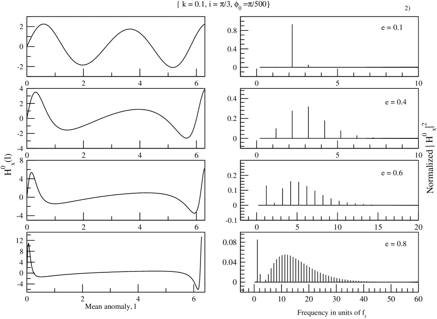
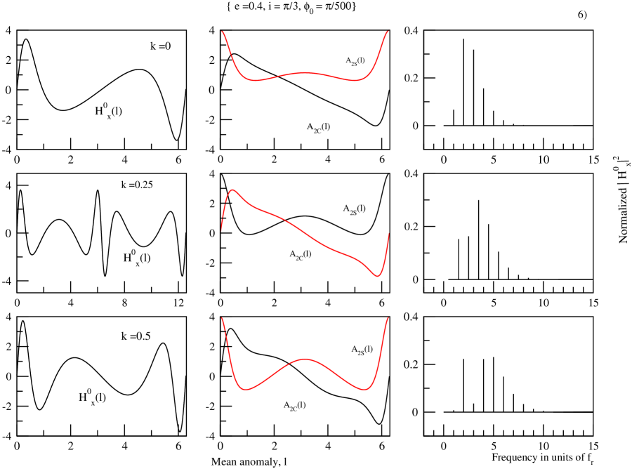
Using the above inputs, we plot the time-domain waveforms $H^{0}_{\times,+}(l)$ and the associated normalized relative power spectrum $\frac{(H^{(0)}_{{\times},{+}})^{j}}{\sum_{j}\,(H^{(0)}_{{\times},+})^{j}}$ in Figs. (2)-(6). The combined influence of the orbital parameters like eccentricity $e$, periastron advance parameter $k$ and orbital inclination $i$, on the time-domain waveform and the associated power spectrum of the Newtonian $h_{\times}$ and $h_{+}$ using Newtonian accurate orbital motion is summarized below.
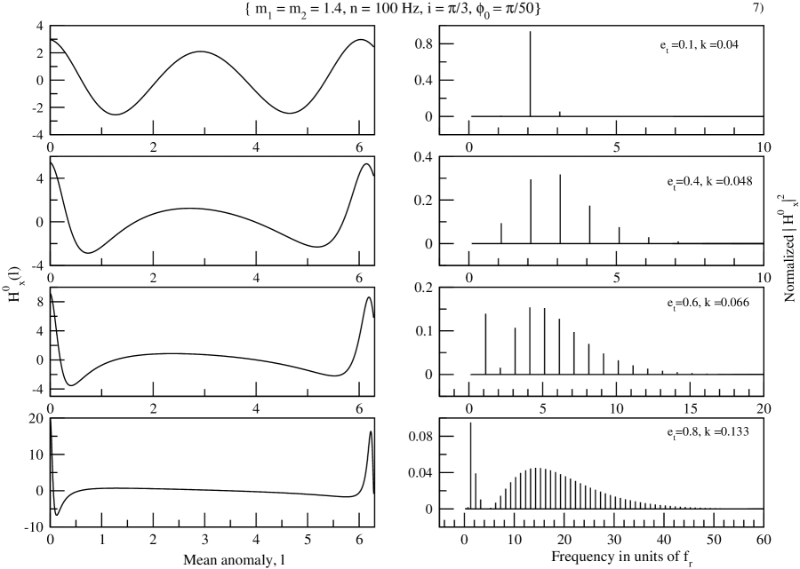
  • $\bullet$

    Eccentricity, $e$ .

    The effects of $e$ on $H^{0}_{\times}$ are explored in Fig. (2). In the limit of low values of eccentricity $e$, as expected, the dominant contribution to the power spectrum, comes from the second harmonic. However, as the eccentricity $e$ increases, higher harmonics appear in the spectrum with comparable strengths. For a given value of the periastron advance $k$ and inclination angle $i$, the position of the dominant harmonic changes as the value of $e$ increases. The shape of the waveform also changes significantly as we increase $e$. For moderate and high values of $e$ there is a stronger burst of radiation near values $l=0$ and $2\,\pi$ corresponding to the periastron passage, since near the periastron, the two masses are closest to each other and their relative velocity is a maximum. In the frequency domain this results in the broad peak containing many frequencies. The line feature in the frequency domain on the other hand corresponds to the average orbital motion of the binary.

  • $\bullet$

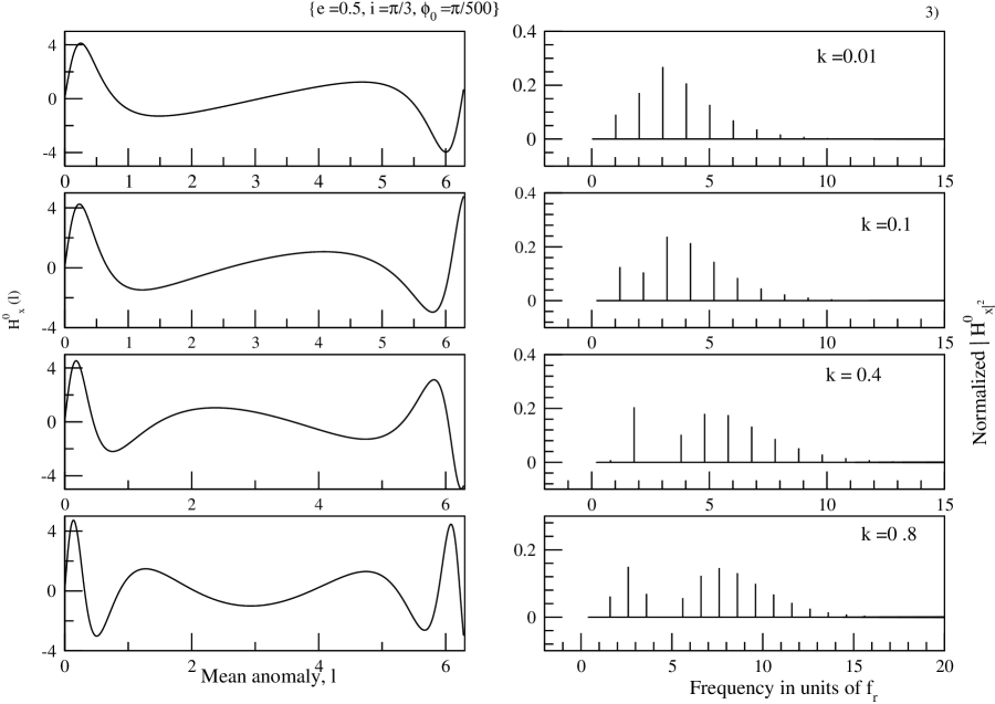
    The ‘arbitrary’ periastron advance parameter, $k$.  The observation made here are based on Fig. (3). A careful inspection of $H^{0}_{\times,+}(l)$ with $k\neq 0$ indicates that in general they are not $2\,\pi$ periodic. This is expected as $k$ is a measure of the angle of return to the periastron. As mentioned earlier, in the power spectrum, the main effect of including an arbitrary $k$ is a ‘splitting’ and subsequent ‘shifting’ of the position of each spectral line from its integer multiple value in units of $f_{r}$, the radial frequency. The shift is appreciable for medium and high eccentricities and leads to a shift of the dominant harmonic in the spectrum.
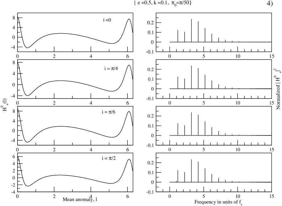
  • $\bullet$

    Orbital inclination, $i$.  A change in the orbital inclination changes only the magnitude of $H^{0}_{\times}$ and its power spectrum, keeping the relative distribution of spectral lines the same. This is easy to see as the dependence of orbital inclination angle $i$ is easily factored out in the expression for $h_{\times}$. However, the shape of $H^{0}_{+}$ and its power spectrum is influenced by $i$ as seen in Fig. (4).

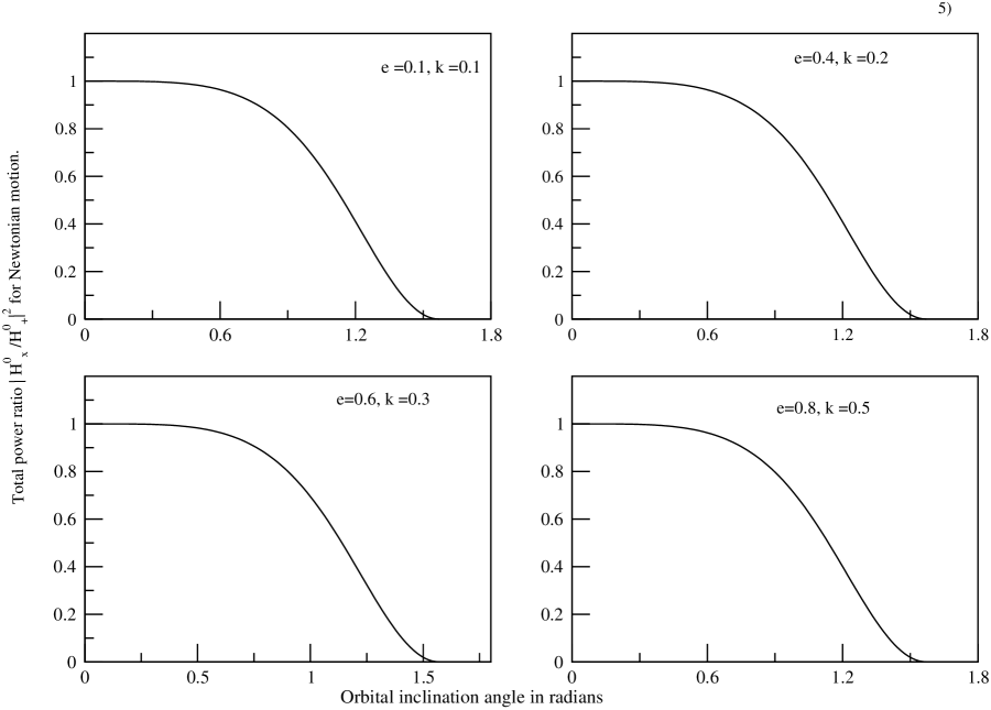
    If the polarizations of the gravitational wave $h_{\times}$ and $h_{+}$ are available, the orbital inclination can be inferred by computing the ratio of the total power measured in each polarization. For circular orbits, the result analytically follows since ${|h^{N}_{\times}|^{2}\over|h^{N}_{+}|^{2}}$ is only a function of $i$ and is given by ${4\,\cos^{2}i\over(1+\cos^{2}i)^{2}}$. In the general eccentric case, to explore this, we plot $\frac{|h^{N}_{\times}|^{2}}{|h^{N}_{+}|^{2}}$ as a function of $i$ for various values of the $e$ and $k$ in Fig. (5). The plots are identical for different values of $e$ and $k$ but vary with the inclination angle providing support for the claim made in the beginning of this paragraph.

Even though in general, an arbitrary periastron advance parameter $k$ at Newtonian order destroys the $2\pi$-periodicity of $H^{0}_{\times,+}(l)$, we may choose $k$ values exactly equal to 00 or $0.5$ so that $H^{0}_{\times}(l)$ is still $2\,\pi$ periodic. These particular values of $k$ allow us to perform useful numerical checks on our analytical procedure. In this case, we can compute the power spectrum directly from $H^{0}_{\times}(l)$ by numerically implementing the Discrete Fourier Transform of Eqs. (III). We can also implement Eq. (445) to obtain the power spectrum, after adding contributions from various $\bar{C}_{j}$ and $\bar{S}_{j}$ to a given harmonic, which is now some integer multiple of the radial frequency, $f_{r}$. The results are displayed in Fig. (6). For better comparison, in these figures, we normalize relative to the power in the dominant harmonic rather than relative to the total power as in other figures. We next, choose $k=0.25$, so that now $H^{0}_{\times}(l)$, is now $4\,\pi$ periodic. Again, comparison with the power spectrum computed directly from Eq. (III) and via Eq. (445) is possible. The results for $k=0,0.25$ and $0.5$ via these two methods are compared and found to be identical up to numerical errors as seen in Fig. (6), providing important checks on our analysis and routines that compute the one sided power spectrum via Eq.(445). We observe a similar behavior for $H^{0}_{+}$.

B The 2PN accurate orbital description

The spectral analysis discussed in the previous section may be extended to 2PN accurate orbital motion with minor technical modifications. The expressions for ${\rm W}(l)$ and $\lambda$ in the $\phi=\lambda+{\rm W}(l)$ split are now given by Eqs. (II B). Moreover, the orbital elements appearing in $H^{(0)}_{\times}$ and $H^{(0)}_{+}$ are now 2PN accurate. These changes will modify expressions for $S_{j}$, $C_{j}$ in Eq. (445) for the ‘${\times}$’ waveform and the corresponding expressions for the ‘$+$’ waveform.

To implement the 2PN accurate spectral analysis, we note the following: First, at the 2PN level the simpler approach to obtain the $u(l)$ relation, connecting the mean and eccentric anomalies, is to numerically solve for $u(l)$ from Eq. (II B) because 2PN accurate analytic expression for $u(l)$ similar to Eq. (446) is not available in the literature. However, we may employ Eq.(447) with $e_{\phi}$ in the place $e$ to get $v-u$ at 2PN order. This is because in the generalized quasi-Keplerian representation, the relation connecting true anomaly $v$ to eccentric anomaly $u$ has the same structural form as for the Keplerian case. Secondly, there are post-Newtonian corrections to the relations connecting $e_{r}$ and $e_{\phi}$ to $e_{t},m_{1},m_{2}$ and $n$. In our analysis, only those values of $e_{t}$ are considered which lead to $e_{\phi},e_{r}$ less than one. Finally, in this 2PN accurate orbital description, the periastron precession constant $k$ is no longer arbitrary but uniquely determined by $m_{1},m_{2},n$ and $e_{t}$ as given by in Eq. (II B).

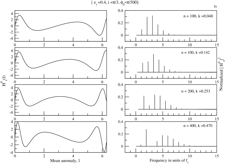
We explore the effects of 2PN accurate orbital motion on the power spectrum for ‘${\times}$’ polarization in Figs. (7), and (8). In Fig. (7), we explore the influence of $e_{t}$ on the relative power spectrum and the behavior is qualitatively similar to the Newtonian case. We explore, in Fig. (8), the effect of changing values for $k$ by varying $m_{1},m_{2}$ and $n$ after fixing the value of $e_{t}$. We see that the behavior is similar to the Newtonian case when we vary values of $k$ for a given $e$. This is required as at 2PN order, for a given $e_{t}$, $k$ is uniquely determined by $m_{1},m_{2}$ and $n$. However, there are quantitative differences in that positions and strengths of various harmonics are different in the Newtonian and the 2PN cases.

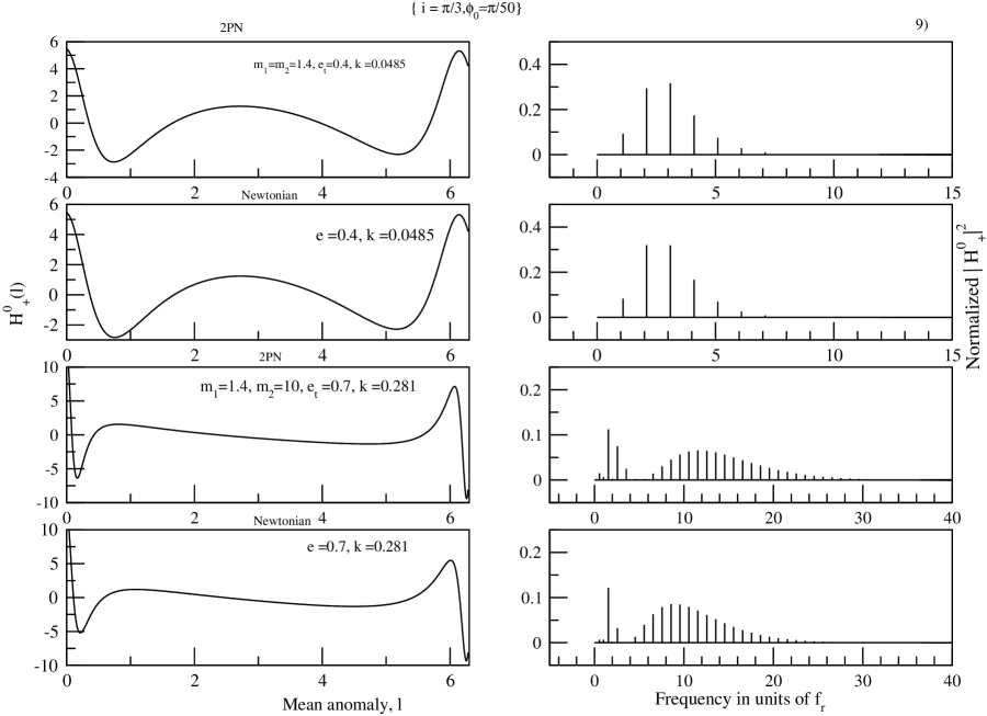
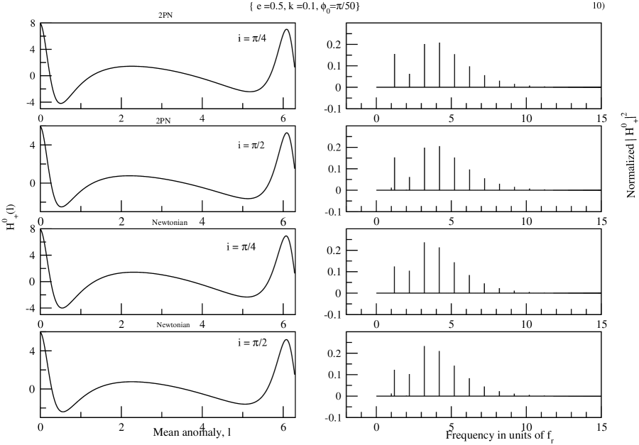
A quantitative comparison between the spectral analysis with Newtonian and 2PN motion is presented in Figs. (9) and (10). Note that we can perform this comparison as we are using scaled polarization waveforms, $H^{0}_{\times}$ and $H^{0}_{+}$. In Fig. (9), we plot both $H^{0}_{+}(l)$ and its power spectrum using Newtonian and 2PN accurate orbital motion. We choose the arbitrary parameter $k$, introduced in the Newtonian case to match the 2PN accurate $k$ associated with the generalized quasi-Keplerian representation. In this manner, we force orbital elements for Newtonian and 2PN dynamics to be the same. Though, qualitatively similar, the plots for the Newtonian and the 2PN orbital motion are quantitatively different in that strengths of spectral lines are different by a few parts in thousand in most cases.

Finally, in Fig. (10), we plot $H^{0}_{+}(l)$ and its power spectrum as a function of orbital inclination angle for Newtonian and 2PN accurate orbital motion. The value of $k$ for the Newtonian runs are again chosen so that it is comparable to the actual 2PN accurate $k$ value. It is clear from these figures that inclusion of PN corrections to orbital motion changes distribution of spectral lines, though the position of the dominant (maximum amplitude) harmonic is roughly the same. This figure also shows how the orbital inclination angle $i$ slowly modulates the spectral lines for Newtonian and 2PN orbital motion.

IV Conclusions

A Summary of results

In this paper we have computed all the ‘instantaneous’ 2PN contributions to $h_{+}$ and $h_{\times}$ for two compact objects of arbitrary mass ratio moving in elliptical orbits, using 2PN corrections to $h^{TT}_{ij}$ and the generalized quasi-Keplerian representation for the 2PN motion. The expressions for $h_{+}$ and $h_{\times}$ obtained here represent gravitational radiation from an elliptical binary during that stage of inspiral when orbital parameters are essentially the same over a few orbital periods, in other words when the gravitational radiation reaction is negligible. We investigate the effect of eccentricity, advance of periastron and orbital inclination on the power spectrum of the Newtonian part of $h_{+}$ and $h_{\times}$. The 2PN accurate generalized quasi-Keplerian representation is used in conjunction with two angular variables $l$ and $\lambda$ chosen to facilitate the subsequent analysis of the waveform evolving under gravitational radiation reaction. These expressions thus form the first step in the direction of obtaining ‘ready-to-use’ theoretical templates for inspiralling compact bodies moving in quasi-elliptical orbits.

B Future directions

There are several issues that remain open for further investigation. We list them below.

  1. 1.

    The next natural step is to obtain evolving $h_{\times}$ and $h_{+}$, when lowest order radiation reaction effects are included in the evolution of orbital elements. This is currently under investigation [14].

  2. 2.

    There are tail contributions to $h_{+}$ and $h_{\times}$ appearing at 1.5PN and 2PN orders. Though the formal expressions for tail terms are available in [32, 10], they need to be written down in a form similar to ‘instantaneous’ contributions to $h_{+}$ and $h_{\times}$ presented in this paper.

  3. 3.

    After computing ‘ready-to-use’ search templates for inspiralling binaries in ‘quasi-elliptical’ orbits, one will be able to address a variety of data analysis issues related to the observations of gravitational radiation from eccentric binaries in great detail. These could include defining a ‘restricted post-Newtonian’ waveform, extending to 2PN accuracy the effect of eccentricity on detection discussed in [29, 53] where currently the orbital dynamics is restricted to leading Newtonian order only.

  4. 4.

    Finally, the analysis of the present paper may be useful for detecting continuous gravitational waves from known sources in binaries. Recent analysis [25] employing a Keplerian representation for the binary’s orbital motion indicates that the computational cost required to search such sources is affordable. The present analysis and [14] may be crucial for including the relevant relativistic effects.

Note added in proof:   We observe that the results of our spectral analysis are in agreement with [30] for low values of $k$. Since the effect of the periastron precession on the amplitude of spectral lines is not fully taken into consideration in [30], the strength of the spectral lines in our analysis differs from theirs, for high values of $k$. It should be noted that for a given $k$, both methods give the same frequency shift for spectral lines, for all values of $k$.

Acknowledgments

We thank T. Damour for discussions and insights that led us towards the final form for the gravitational wave polarizations presented here and D. Bhattacharya for critical comments clarifying the implementation and results of the spectral analysis of waveforms. We are grateful to L. Blanchet, S. Iyer, B. S. Sathyaprakash, G. Schäfer and B. Schutz for their comments at different stages of this project. One of us (AG) is supported in part by NSF grant No. PHY 96-00049 and is grateful to C. M. Will for encouragement.

REFERENCES

  • [1] The easiest way to obtain brief or detailed information about earth and space based interferometers is to visit their respective web sites which are given below :
    LIGO : http://www.ligo.caltech.edu; VIRGO : http://www.virgo.infn.it; GEO600 : http://www.geo600.uni-hannover.de ; TAMA : http://tamago.mtk.nao.ac.jp.
  • [2] LISA : http://lisa.jpl.nasa.gov.
  • [3] C. Cutler, L. S. Finn, E. Poisson, and G. J. Sussmann, Phy.  Rev.  D47, 1151 (1993).
  • [4] C. Cutler and É. E. Flanagan, Phys. Rev. D 49, 2658 (1994).
  • [5] Currently, there are three independent groups, employing three different approaches, tackling various issues at the 3PN order. The first group uses the Arnowitt-Deser-Misner (ADM) canonical approach and their results may be found in:
    P. Jaranowski and G. Schäfer, Phys. Rev. D 57, 5948 (1998); ibid D 57, 7274 (1998); ibid D 60, 1240003 (1999); T. Damour, P. Jaranowski and G. Schäfer, Phys. Rev. D 62, 021501; ibid D 62, 044024; ibid D 62, 084011 (2000). Recently, undetermined parameters appearing in the reduced 3PN Hamiltonian has been fixed by dimensional regularisation in T. Damour, P. Jaranowski and G. Schäfer, gr-qc/0105038.
    The second group employs harmonically relaxed Einstein equations and relevant results are in: L. Blanchet, G. Faye and B. Ponsot, Phys. Rev.  D 58 124002 (1998); L. Blanchet and G. Faye, Phys. Lett., 271, 58 (2000); L. Blanchet and G. Faye, gr-qc/0004009; gr-qc/0006100; gr-qc/7051; V. Andrade, L. Blanchet and G. Faye, Class. Quant Grav.  18, 753, 2001.
    The third group is adapting a method, called DIRE, for Direct Integration of Relaxed Einstein Equations and results are in: M. E. Pati and C. M. Will, gr-qc/0007087, Phys. Rev.  D 62 124015, (2000);
  • [6] L. Blanchet, B. R. Iyer and B. Joguet, gr-qc/0105098, Phys. Rev.  D (To appear); L. Blanchet, G. Faye, B. R. Iyer and B. Joguet, gr-qc/0105099.
  • [7] T. Damour, B. R. Iyer, and B. S. Sathyaprakash, Phys.  Rev.  D 57, 885 (1997). T. Damour, B. R. Iyer, and B. S. Sathyaprakash, Phys. Rev. D 62, 084036 (2000), A. Buonanno and T. Damour, Phys.Rev. D 62, 064015 (2000), T. Damour, B.R. Iyer, and B.S. Sathyaprakash, Phys.Rev. D 63, 044023 (2001).
  • [8] L. Blanchet, B.R. Iyer, C. M. Will and A. G. Wiseman, Class. Quantum Grav. 13, 575 (1996).
  • [9] L. Blanchet, T. Damour, B.R. Iyer, C. M. Will and A. G. Wiseman, Phys. Rev. Lett. 74, 3515 (1995).
  • [10] L. Blanchet, T. Damour, and B. R. Iyer, Phys. Rev. D 51, 5360 (1995).
  • [11] C. M. Will and A. G. Wiseman, Phys. Rev. D 54, 4813 (1996).
  • [12] L. Blanchet, Phys. Rev. D 54, 1417 (1996)
  • [13] LIGO/LSC Algorithm Library, http://www.lsc-group.phys.uwm.edu/lal/index.html.
  • [14] T. Damour, A. Gopakumar and B. R. Iyer (Work in progress).
  • [15] É. E. Flanagan and S. A. Hughes, Phys.  Rev.  D 57, 4535 (1998).
  • [16] V.M. Lipunov, K.A. Postnov, and M.E. Prokhorov, New Astron. 2, 43 (1997);
  • [17] M. C. Miller and D. P. Hamilton, Production of Intermediate-Mass Black Holes in Globular Clusters, astro-ph/0106188.
  • [18] S.P. Zwart and S. McMillan, Astrophys. J. 528, L17 (2000).
  • [19] S. L. Shapiro and S. A. Teukolsky, Astrophys. J. 292, L41 (1985); G. D. Quinlan and S. L. Shapiro, Astrophys. J. 321, 199 (1987).
  • [20] J. Levin, Phys. Rev. Lett. 16, 3515 (2000), gr-qc/0010100; N. J. Cornish, Phys. Rev. Lett. 85, 3980 (2000). S. A. Hughes, Phys. Rev. Lett. 85, 5480 (2001);
  • [21] LISA Mission Concept Study, JPL Pub. 97-16, March 1998, available from http://lisa.jpl.nasa.gov/documents.html. For recent papers dealing with coalescence of compact binaries which is relevant for LISA and where eccentricity is important see: T. Ebisuzaki, et.al, Missing Link Found? — The “runaway” path to supermassive black holes, astro-ph/0106252; V.B. Ignatiev, A.G.Kuranov K.A. Postnov and M.E. Prokhorov, Gravitational wave background from coalescing compact stars in eccentric orbits , astro-ph/0106299.
  • [22] T. Nakamura, M. Sasaki, T. Tanaka and K. S. Thorne, Astrophys. J. 487, L139 (1997).
  • [23] W. A. Hiscock, Astrophys. J. 509, L101 (1998).
  • [24] K. Ioka, T. Tanaka, and T. Nakamura, Phys. Rev.  D 60, 083512,(1999).
  • [25] S. V. Dhurandhar and A. Vecchio, gr-qc/0011085.
  • [26] C. W. Lincoln and C. M. Will, Phys. Rev. D 42, 1123 (1990).
  • [27] T. Damour and N. Deruelle, C. R. Acad. Sci. Paris 293, 537 (1981); 293, 877 (1981);
  • [28] T. Damour and N. Deruelle, Ann. Inst. Henri Poincare Phys. Theor. 43, 107 (1985).
  • [29] C. Moreno-Garrido, J. Buitrago and E. Mediavilla, Mon. Not. R. Astron. Soc. 266, 16 (1994).
  • [30] C. Moreno-Garrido, J. Buitrago and E. Mediavilla, Mon. Not. R. Astron. Soc. 274, 115 (1995).
  • [31] W. Junker and G. Schäfer, Mon. Not. R. Astron. Soc. 254, 146 (1992).
  • [32] L. Blanchet and G. Schäfer, Class. Quantum Grav. 10, 2699 (1993).
  • [33] L. Blanchet, Phys. Rev. D 51, 2559 (1995).
  • [34] Black Hole perturbation results relevant to the generation of gravitational radiation is reviewed by Y. Mino, M. Sasaki, M. Shibata, H. Tagoshi, T. Tanaka, Prog. Theor. Phys Ṡuppl 1̇28, 1, (1997).
  • [35] L. E. Kidder, C. M. Will, and A. G. Wiseman, Phys. Rev. D 47, R4183 (1993).
  • [36] T. A. Apostolatos, C. Cutler, G. J. Sussman, and K. S. Thorne, Phys. Rev. D 49, 6274 (1994).
  • [37] L. E. Kidder, Phys. Rev. D 52, 821 (1995).
  • [38] B. J. Owen, H. Tagoshi, and A. Ohashi, Phys. Rev. D 57, 6168 (1997); H. Tagoshi, A. Ohashi and B. J. Owen, gr-qc/0010014.
  • [39] A. Gopakumar and B. R. Iyer, Phys. Rev. D 56, 7708 (1997).
  • [40] T. Damour and N. Deruelle, Ann. Inst. Henri Poincare Phys. Theor. 44, 263 (1986).
  • [41] T. Damour and G. Schäfer, CR Acad. Sci. II 305, 839, (1987).
  • [42] T. Damour and G. Schäfer, Nuovo Cimento B 101, 127 (1988).
  • [43] G.. Schäfer and N. Wex, Phys. Lett. 174 A, 196, (1993); erratum 177, 461.
  • [44] N. Wex, Class. Quantum Gr. 12, 983, (1995).
  • [45] T. Damour, Phys. Rev. Lett. 51, 1019, (1983).
  • [46] T. Damour and G. Schäfer, Gen. Rel. Grav.  17, 879, (1985).
  • [47] Following conventions used in celestial mechanics, the orbital phase was measured from the line of nodes in [8], which coincide with $+$ve y-axis in Fig. 1. However, we measure the orbital phase from $+$ve x-axis. This is because the 2PN accurate generalized quasi-Keplerian parametrization is given in the usual polar coordinates, $r$ and $\phi$. The angular variable $\phi$, appearing in polar coordinates, is usually measured from $+$ve x-axis as shown in Fig. 1. This is why we use angular transformation relation $\phi\equiv\lambda+{\rm W}(l)=\left(\phi_{\rm BIWW}-{\pi\over 2}\right)$ to compare circular limit of our expressions for $h_{+}$ and $h_{\times}$ with those presented in [8], modulo the tail terms.
  • [48] MAPLE, Waterloo Maple Software, Waterloo, Ontario, Canada.
  • [49] At Newtonian order, units for $f_{r}$ is arbitrary. This is because the only relevant parameters $e$ and $k$ don’t define $n$ uniquely when we vary $l=n\,(t-t_{0})$ from 00 to $2\,\pi$ to get $H^{0}_{\times,+}(l)$. However, at 2PN order, units for $f_{r}$ is Hertz, since to get realistic values of $k$, defined in terms of $m_{1},m_{2},n$ and $e$, we choose $f_{r}$ in Hertz along with $m_{1}$ and $m_{2}$ in solar mass units.
  • [50] We consider $k=0,0.25,0.5$ values as they make $H^{(0)}_{\times}(l)$ periodic within a couple of orbits. Note that $k=0$ may be thought to represent a binary with vanishing periastron advance.
  • [51] W.H. Press, S. Teukolsky, W.T Vetterling and B.P Flannery, Numerical Recipes: The art of scientific computing (Cambridge University Press, Cambridge, England, 1992).
  • [52] D. Brouwer and G. M. Clemence, Methods of Celestial Mechanics, Academic Press, 1961.
  • [53] K. Martel and E. Poisson, Phys.Rev. D60, 124008, (1999); M. Benacquista, Detecting Eccentric Globular Cluster Binaries with LISA, astro-ph/0106086.
Refer to caption
FIG. 1.: The orientation of unit vectors, which defines $\times$ and $+$ polarization waveforms. The unit vectors p and q are the gravitational wave’s principal axes with ${\bf q}=$ N $\times$ p. Note that N is a unit vector lying along the radial direction to the detector and p lies along the line of nodes. The Newtonian angular momentum vector ${\bf L}=\mu\,{\bf r}\,\times\,{\bf v}$ is normal to the orbital plane and helps to define orbital inclination angle $i$. In this paper, the origin for $\phi=\lambda+{\rm W}$ is $+$ve x-axis, hence it is related to $\phi_{\rm BIWW}$ by $\phi=\phi_{\rm BIWW}-{\pi\over 2}$.
Refer to caption
FIG. 2.: Plots for scaled GW polarization waveform, $H^{0}_{\times}$ as a function of the mean anomaly, $l$ and the corresponding normalized relative power spectrum using Newtonian orbital motion, for various values of eccentricity $e$. Note in $H^{0}_{\times}(l)$ a ‘burst’ of GW emission near periastron passage and a shift in the position of the dominant harmonic in the power spectrum as $e$ increases. In the Fourier domain, the former results in a broad frequency rich peak. In all panels, the (arbitrary) periastron precession constant and the orbital inclination angle take values $0.1$ and ${\pi\over 3}$ respectively.
Refer to caption
FIG. 3.: The configuration is similar to Fig.2, but in the panels, $k$, the (arbitrary) periastron precession constant is varied for fixed eccentricity $e=0.5$ and orbital inclination angle $i={\pi\over 3}$. Note the splitting and shifting of spectral lines from integer multiple values of $f_{r}$ as $k$ is increased.
Refer to caption
FIG. 4.: Plots of scaled GW polarization waveform, $H^{0}_{+}$ as a function of mean anomaly, $l$ and its corresponding normalized relative power spectrum for Newtonian orbital motion, when the orbital inclination angle $i$ is varied. In all frames, eccentricity $e=0.5$ and periastron precession constant, $k=0.1$.
Refer to caption
FIG. 5.: The ratio of the total power measured in $\times$ and $+$ polarization for Newtonian motion as a function of orbital inclination angle $i$ for various values of periastron precession constant $k$ and eccentricity $e$. From the plots, it is clear that the ratio is independent of the orbital elements like $e$ and $k$.
Refer to caption
FIG. 6.: Plots of $H^{0}_{\times}{l}$, ${\rm A_{2C}}(l),{\rm A_{2S}}(l)$ as a function of mean anomaly, $l$ and their relative power spectra constructed using Eq. (445) and directly using $H^{0}_{\times}(l)$. The orbital motion is Newtonian accurate and we employ certain specific values of $k=0,0.5$ and $0.25$. The relative power spectra, plotted in third column, are numerically identical, hence indistinguishable. Note that plots in second column are always $2\,\pi$ periodic, while those in the first column are $2\,\pi,2\,\pi$ and $4\,\pi$ periodic for $k=0$, $k=0.5$ and $k=0.25$ respectively
Refer to caption
FIG. 7.: Plots for scaled GW polarization waveform, $H^{0}_{\times}(l)$ and corresponding normalized relative power spectrum using 2PN accurate orbital motion, for various values of $e_{t}$. Unlike in Fig. 2, the value of $k$ cannot be independently chosen since it is uniquely determined by the values of $m_{1},m_{2},n$ and $e_{t}$. The observations from plots are similar to Fig. 2, as variation in $k$ is small compared to that in $e_{t}$. In all frames, $m_{1}$ = $m_{2}$ = 1.4 $M_{\odot}$, orbital inclination angle $i={\pi\over 3}$ and mean motion $n=100\,$ radians per second.
Refer to caption
FIG. 8.: The configuration is similar to Fig. 7, but in the panels we vary masses and mean motion to get the different values of $k$, rather than $e$. For all plots $e_{t}=0.4$ and $i={\pi\over 3}$. Qualitatively, conclusions are similar to Fig. 3. Unit for $n$ will be radians per second.
Refer to caption
FIG. 9.: Plots of scaled GW polarization waveform, $H^{0}_{+}(l)$ and corresponding normalized relative power spectrum for Newtonian and 2PN accurate orbital motion. Given $e_{t}$, we vary values for $m_{1}$, $m_{2}$ and $n$, to make $k$ values the same in the 2PN and the Newtonian accurate orbital motion. In all frames, orbital inclination angle is ${\pi\over 3}$. Panels in the 2nd and 4th rows are for Newtonian orbital motion, whereas panels in the 1st and 3rd rows are for 2PN accurate orbital motion. We see minor quantitative differences in the position and strength of spectral lines at these two orders.
Refer to caption
FIG. 10.: Plots for the scaled GW polarization waveform, $H^{0}_{+}$ as a function of mean anomaly, $l$ and the corresponding normalized relative power spectrum using 2PN and Newtonian accurate orbital motion. We vary the orbital inclination angle, $i$ keeping other orbital elements constant at Newtonian and 2PN level. Conclusions are similar to Fig. 4.