Isometric embeddings of black hole horizons in three-dimensional flat space

Abstract

The geometry of a two-dimensional surface in a curved space can be most easily visualized by using an isometric embedding in flat three-dimensional space. Here we present a new method for embedding surfaces with spherical topology in flat space when such a embedding exists. Our method is based on expanding the surface in spherical harmonics and minimizing for the differences between the metric on the original surface and the metric on the trial surface in the space of the expansion coefficients. We have applied this method to study the geometry of back hole horizons in the presence of strong, non-axisymmetric, gravitational waves (Brill waves). We have noticed that, in many cases, although the metric of the horizon seems to have large deviations from axisymmetry, the intrinsic geometry of the horizon is almost axisymmetric. The origin of the large apparent non-axisymmetry of the metric is the deformation of the coordinate system in which the metric was computed.

]

I Introduction

In the past few years, important progress has been made in the development of fully three-dimensional (3D) numerical relativity codes. These codes are capable of simulating the evolution of strongly gravitating systems, such as colliding black holes and neutron stars, and can provide important physical information about those systems such as the gravitational waves they produce. The codes also allow one to locate and track the evolution of apparent and event horizons of black holes that might exist already in the initial data or might form during the evolution of the spacetime. However, since the location of such horizons is obtained only in coordinate space, one typically has little information about the real geometry of those surfaces. One can, for example, obtain very similar shapes in coordinate space for horizons that are in fact very different (see for example the family of distorted black holes studied in [1]; their coordinate locations are very similar, but their geometries are quite different). The most natural way to visualize the geometry of a black hole horizon, or of any other surface computed in some abstract curved space is to find a surface in ordinary flat space that has the same intrinsic geometry as the original surface. The procedure of finding such a surface is called embedding the surface in flat space.

It is a well known fact [2] that any two dimensional surface is locally embeddable in flat 3D space. Global embeddings of a surface, on the other hand, might easily not exist, and even when they do they are not easy to find. However, several methods have been proposed in the past for computing partial (or global) embeddings of surfaces when such embeddings exist.

Partial embeddings of a slice through the Misner initial data for colliding black holes [3] have been computed for example in [4]. The method used to find such embeddings starts from the metric of the original surface written in terms of some local coordinates $(u,v)$:

$$ds^{2}=Edu^{2}+2Fdudv+Gdv^{2}\,.$$ (1)

One then introduces embedding functions $X(u,v)$, $Y(u,v)$ and $Z(u,v)$ such that

$$dX^{2}+dY^{2}+dZ^{2}=ds^{2}=Edu^{2}+2Fdudv+Gdv^{2}\,,$$ (2)

which implies

$$E = X_{,u}^{2}+Y_{,u}^{2}+Z_{,u}^{2}\,,$$ (3)

$$F = X_{,u}X_{,v}+Y_{,u}Y_{,v}+Z_{,u}Z_{,v}\,,$$ (4)

$$G = X_{,v}^{2}+Y_{,v}^{2}+Z_{,v}^{2}\,.$$ (5)

The above system of non-linear first order partial differential equations is not of any standard type. In order to solve it one can use a method originally proposed by Darboux. This leads to a single non-linear second order partial differential equation for $Z(u,v)$ known as the Darboux equation. The character of the Darboux equation depends on the sign of the Gaussian curvature $K$ of the surface and on the orientation of the embedding at the point of integration as follows: for $K\geq 0$ the equation is elliptic, for $K\leq 0$ it is hyperbolic and it has parabolic character both if $K=0$ or if the surface is vertical. For the Misner geometry, the curvature is always negative and the Darboux equation is hyperbolic. It can then be rewritten by using the characteristics as coordinates, and solved as a Cauchy problem given appropriate initial data. Once the Darboux equation has been solved for $Z(u,v)$, the remaining equations can be integrated to give $X(u,v)$ and $Y(u,v)$.

This method is not appropriate for embedding surfaces that have both regions with $K>0$ and regions with $K<0$. The reason for this is that the Darboux equation one has to integrate is elliptic for $K>0$ and hyperbolic for $K<0$. This means that for such surfaces the Darboux equation will change type and its integration will become very difficult. This will typically be the case for surfaces with spherical topology, such as black hole horizons, which will always have some regions of positive curvature, and may well have regions of negative curvature too.

One of the first studies of the intrinsic geometry of rotating black hole horizon surfaces was carried out by Smarr [5]. There it was show, by direct construction of the embedding from the analytic Kerr metric, that while the horizon of a Schwarzschild black hole is spherical, for rotating black holes the horizon has an equatorial bulge, a satisfying and intuitive result that reinforces the notion that geometric studies of black hole horizons can add physical insight. The equatorial bulge can be characterized by an oblateness factor that is uniquely determined by the ratio $a/m$, where $m$ is the mass of the black hole and $a$ its rotation parameter. It was also shown that for rapidly rotating black holes, with $a/m>\sqrt{3}/2$, the Gaussian curvature becomes negative near the poles, and the surface is not embeddable in Euclidean space, as it is “too flat”!

Extending on this work, using a direct constructive embedding method described below, a number of studies were made of distorted, rotating, and colliding black hole horizons in axisymmetry [6, 1, 7, 8, 9, 10] where it was shown that embeddings are very useful tools to aid in the understanding of the dynamics of black holes. For example, distorted rotating black hole horizons were found to oscillate, about their oblate equilibrium shape, at their quasi-normal frequency. The recent work on isolated horizons [11, 12, 13, 14] shows how geometric measurements of the horizon can be used to determine, for example, the spin of a black hole formed in some process, and other physical features.

However, in the absence of axisymmetry, the problem of constructing an embedding for a black hole horizon becomes much more difficult. One approach to compute such embeddings of horizons in 3D spacetimes has been suggested by H.-P. Nollert and H. Herold [15]. They consider a triangular wire frame on the original surface and compute the distances between each point and its neighbors using the intrinsic metric of the surface. They then consider a network with the same topology in flat space and try to solve the system of equations

$$|{\bf r}_{i}-{\bf r}_{j}|=d_{ij}\,,$$ (6)

where ${\bf r}_{k}$ represents the position vector of the $k^{\text{th}}$ point in flat space and $d_{ij}$ represents the distance between the points $P_{i}$ and $P_{j}$ computed on the original surface. If necessary, they refine the grid until they reach a desired accuracy.

The approach of Nollert and Herold seems very natural, but is has the serious drawback that it does not always converge to the correct solution. The reason for this is that the method imposes constraints only on the distances between points, but it does not guarantee that the final surface will be smooth. There are in fact multiple solutions to the system of equations, and for most such solutions the resulting embedding is not smooth. For example, if one tries to embed a simple sphere, this method might indeed converge to the sphere, but it might also converge to the surface one obtains if one cuts the top of the sphere, turns its up-side down and glues it back. The distances between point are the same in both surfaces, but only one of them is smooth.

The method for computing embeddings that we present in this paper is based on a spectral decomposition of the surface in spherical harmonics written in a non-trivial mapping of the coordinate system. We search for the embedding by minimizing for the difference between the metric of the original surface and that of our trial embedding in the space of the coefficients of the spherical harmonics and of the coordinate mappings. Since we use a decomposition of the surface in spherical harmonics, the surface is guaranteed to be smooth. By increasing the number of spherical harmonics used in the decomposition of the physical surface, one can get as close to the correct embedding as desired.

II Our Method

The intrinsic geometry of any surface is completely determined by its metric. To construct the embedding of a given surface $S$, one needs to find a surface $S^{\prime}$ in flat space that has the same metric as $S$ in an appropriate coordinate system. It is important to stress here the fact that finding the embedding surface $S^{\prime}$ also requires that one finds an appropriate mapping of the original coordinate system in the surface $S$ to a new coordinate system in the surface $S^{\prime}$ in which the two metrics are supposed to agree.

A A Direct Method for Horizon Embeddings in Axisymmetry

Before describing our new method, it is instructive to describe a simple and direct method for axisymmetric embeddings of horizons, used by a number of authors to study the physics of dynamic black holes [16, 1, 7, 8, 9, 10, 17].

For the case of non-rotating, axisymmetric spacetimes (easily generalized to rotation, but restricted here merely for ease of illustration), the 3D metric on a given time slice can be written as

$$ds_{(3)}^{2}=A(\eta,\theta)d\eta^{2}+B(\eta,\theta)d\theta^{2}+D(\eta,\theta)\sin^{2}\theta d\phi^{2}.$$ (7)

The location of the axisymmetric horizon surface is given by the function $\eta=\eta_{s}(\theta)$. The 2D metric induced on the horizon surface is then given by

$$ds_{(2)}^{2}=\left[B+\left(\frac{d\eta_{s}}{d\theta}\right)^{2}A\right]d\theta^{2}+D\sin^{2}\theta d\phi^{2}\,.$$ (8)

Now, the flat metric in cylindrical coordinates $(z,\rho,\psi)$ can be written as

$$ds^{2}=dz^{2}+d\rho^{2}+\rho^{2}d\psi^{2}.$$ (9)

To create an embedding in a 3D Euclidean space, we want to construct functions $z(\theta,\phi),\rho(\theta,\phi)$, and $\psi(\theta,\phi)$ such that we can identify the line elements given by Eqs. (8) and (9), that is, that all lengths be preserved.

Here, we are faced with our first choice about the coordinates used in the embedding, a problem which will be more complex in the general case as we show below. Since the spacetime itself is axisymmetric, it is a natural choice to make the embedding axisymmetric. We choose, then, to construct a surface for a constant value of $\phi=0$, and we then have $z=z(\theta),\rho=\rho(\theta)$, and the resulting embedding will be a surface of revolution about the $z-$axis. Using the obvious mapping between $\psi$ and $\phi$, $\psi=\phi$, it becomes straightforward to derive ordinary differential equations to integrate for $\rho(\theta)$ and $z(\theta)$ along the horizon surface. It is important to emphasize that we have to make a choice about the embedding coordinates, even in this simpler case, as we must in the general case discussed below.

Using this method, embeddings were carried out during the numerical evolution for a variety of dynamic, axisymmetric black hole spacetimes [16, 1, 7, 8, 9, 10, 17]. The evolution of these embeddings were found to be extremely useful in understanding the physics of these systems. We will use some of these results as test cases for the more general method for 3D spacetimes, as detailed in the next section.

B Our General Method for Embeddings in full 3D

Given a coordinate system $\xi^{i}$ ($i,j=1,2)$ on our surface, the first step in looking for an embedding is to find the two dimensional metric $g_{ij}$ of the surface induced by the metric of the three dimensional space $h_{ab}$ ($a,b=1,2,3$) in which it is defined. The general procedure to find such induced metric is to construct a coordinate basis of tangent vectors ${\bf e}_{i}:=\partial_{i}$ on the surface. The induced metric will then be given by

$$g_{ij}(\theta,\phi)={\bf e}_{i}(\theta,\phi)\cdot{\bf e}_{j}(\theta,\phi)=h_{ab}\,e_{i}^{a}\,e_{j}^{b}\,,$$ (10)

where $e_{i}^{a}$ is the component of the vector ${\bf e}_{i}$ with respect to the three dimensional coordinate $x^{a}$.

Since the surfaces we are concerned with in this paper (black hole horizons) have spherical topology, we will assume that the three-dimensional metric $h_{ab}$ is given in terms of spherical coordinates $(r,\theta,\phi)$ defined with respect to some origin enclosed by the surface. Furthermore, we will also assume that the surface is a “ray-body” (Minkowski’s strahlkorper [18], also known as a “star-shaped” region) that is, a surface such that any ray coming from the origin intersects the surface at only one point. Such a property implies that we can choose as a natural coordinate system on the surface simply the angular coordinates $(\theta,\phi)$.

If we take our surface to be defined by the function $r=f(\theta,\phi)$, then it is not difficult to show that the induced metric $g_{ij}$ on the surface will be given in terms of the three-dimensional metric $h_{ab}$ as:

$$g_{\theta\theta} = h_{\theta\theta}+h_{rr}\left(\partial_{\theta}f\right)^{2}+2h_{r\theta}\partial_{\theta}f\,,$$ (11)

$$g_{\phi\phi} = h_{\phi\phi}+h_{rr}\left(\partial_{\phi}f\right)^{2}+2h_{r\phi}\partial_{\phi}f\,,$$ (12)

$$g_{\theta\phi} = h_{\theta\phi}+h_{rr}\,\partial_{\theta}f\partial_{\phi}f+h_{r\phi}\partial_{\theta}f+h_{r\theta}\partial_{\phi}f\,.$$ (13)

Let us now for moment a assume that an embedding of our surface in flat space exists, and let us also introduce a spherical coordinate system $(r_{e},\theta_{e},\phi_{e})$ in flat space. Notice that there is no reason to assume that a point with coordinates $(\theta,\phi)$ in the original surface will be mapped to a point with the same angular coordinates in the embedding. In general, the embedded surface in flat space will be described by the relations

$$r_{e}=r_{e}(\theta,\phi)\,,\quad\theta_{e}=\theta_{e}(\theta,\phi)\,,\quad\phi_{e}=\phi_{e}(\theta,\phi)\,.$$ (14)

A crucial observation at this point is that the angular coordinates $\{\theta,\phi\}$ in the original surface still provide us with a well behaved coordinate system in the embedded surface, only one that does not correspond directly to the flat space angular coordinates $\{\theta_{e},\phi_{e}\}$, but is instead related to them by the coordinate transformations $\theta_{e}=\theta_{e}(\theta,\phi)$ and $\phi_{e}=\phi_{e}(\theta,\phi)$. This means that under the embedding, points with coordinates $(\theta,\phi)$ in the original surface will be mapped to points with the same coordinates $(\theta,\phi)$ in the embedded surface, but different coordinates $(\theta_{e},\phi_{e})$. We then have two natural sets of coordinates in the embedded surface: the ones inherited directly from the original surface through the embedding mapping, and the standard angular coordinates in flat space.

By definition, an embedding preserves distances, so the proper distance between two points in the original surface must be equal to the distance between the two corresponding points in the embedded surface. Since those corresponding points have precisely the same coordinates $\{\theta,\phi\}$, we must conclude that for the embedding to be correct, the components of the metric tensor in both surfaces when expressed in terms of the coordinates $\{\theta,\phi\}$ must be identical. That is, if we call $g^{e}_{ij}$ the metric of the embedded surface, we must have

$$g_{\theta\theta}=g^{e}_{\theta\theta}\,,\quad g_{\theta\phi}=g^{e}_{\theta\phi}\,,\quad g_{\phi\phi}=g^{e}_{\phi\phi}\,.$$ (15)

It is important to stress that the components of the metric in the embedded surface will only be equal to the components of the metric in the original surface if we use the inherited coordinate system, but not if we use the standard angular coordinates in flat space.

Computing the components of the metric in the embedded surface in terms of the inherited coordinate system $\{\theta,\phi\}$, given the embedding relations (14), is not difficult. All one needs to do in practice is consider four points in the original surface with coordinates $P_{1}(\theta,\phi)$, $P_{2}=(\theta+\delta\theta,\phi)$, $P_{3}=(\theta,\phi+\delta\phi)$, $P_{4}=(\theta+\delta\theta,\phi+\delta\phi)$, find their corresponding coordinates $\{r_{e},\theta_{e},\phi_{e}\}$ in flat space using (14), compute their squared distances using the flat space metric, and then solve for the metric components from

$$(\overline{P_{1}P_{2}})^{2} = g^{e}_{\theta\theta}\,d\theta^{2}\,,$$ (16)

$$(\overline{P_{1}P_{3}})^{2} = g^{e}_{\phi\phi}\,d\phi^{2}\,,$$ (17)

$$(\overline{P_{1}P_{4}})^{2} = g^{e}_{\theta\theta}\,d\theta^{2}+g^{e}_{\phi\phi}\,d\phi^{2}+2g^{e}_{\theta\phi}\,d\theta d\phi\,.$$ (18)

Finding the embedding now means finding a mapping (14) such that equations (15) are satisfied everywhere.

Let us consider first the relation between the $(\theta,\phi)$ coordinates on the original surface and the angular coordinates $(\theta_{e},\phi_{e})$ in flat space. Even if these two sets of coordinates are not equal, we can safely assume that there is a one-to-one correspondence between them. Moreover, both are sets of angular coordinates, so they have the same behavior: $\theta$ and $\theta_{e}$ go from 0 to $\pi$, and $\phi$ and $\phi_{e}$ go from 0 to $2\pi$ and are periodic. From these properties, it is not difficult to see that the most general functional relation between both sets has the form

$$\theta_{e}(\theta,\phi) = \theta+\sum_{n=0}^{\infty}b_{n0}\sin(n\theta)$$ (20)

$$+\sum_{n=1}^{\infty}\sum_{m=1}^{\infty}b_{nm}\sin(n\theta)\,\sin(m\phi)\,,$$

$$\phi_{e}(\theta,\phi) = \phi+c_{00}\,\theta+\sum_{n=1}^{\infty}c_{n0}\sin(n\theta)+\sum_{m=1}^{\infty}c_{0m}\sin{m\phi}$$ (22)

$$+\sum_{n=1}^{\infty}\sum_{m=1}^{\infty}c_{nm}\sin(n\theta)\,\sin(m\phi)\,.$$

The second term in the expansion for $\theta_{e}$ represents a general axisymmetric re-mapping of $\theta$, while the third term is required if axisymmetry is not assumed. In the expression for $\phi_{e}$, the second and third terms represent a possible rigid twist of the coordinate system, and the last two terms stand for a general dependence of $\phi_{e}$ on both $\theta$ and $\phi$.

For the radial coordinate $r_{e}$, it is also not difficult to see that one can use a simple expansion in spherical harmonics of the form

$$r_{e}(\theta,\phi)=\sum_{l=0}^{\infty}\sum_{m=-l}^{l}\sqrt{4\pi}\,a_{lm}Y_{lm}(\theta,\phi)\,,$$ (23)

where the overall normalization factor of $\sqrt{4\pi}$ has been inserted so that $a_{00}$ is the average radius of the surface, $a_{10}$ is its average displacement in the $z$-direction, and so on. We will also use a real basis of spherical harmonics, for which $m$ and $-m$ stand for an angular dependence $\cos(m\phi)$ and $\sin(m\phi)$, instead of the complex $\exp(im\phi)$ and $\exp(-im\phi)$.

The metric of the embedded surface will now be completely determined by the set of coefficients $a_{lm}$, $b_{nm}$ and $c_{nm}$. The space of these coefficients can be regarded as a vector space $V$, with any given point in $V$ representing a surface in flat space together with a certain coordinate mapping.

Consider now an embeddable surface $S$ in some arbitrary curved space. It is not difficult to find a real valued function $F$ defined on $V$ that has a global minimum at the point $P\in V$ for which the metric of the embedded surface $S^{e}$ is the same as the metric of the original surface. One such function is

$$F=\int_{\theta=0}^{\pi}\int_{\phi=0}^{2\pi} \left[\,\left(g_{\theta\theta}(\theta,\phi)-g^{e}_{\theta\theta}(\theta,\phi)\right)^{2}\right.$$ (26)

$$+\left(g_{\phi\phi}(\theta,\phi)-g^{e}_{\phi\phi}(\theta,\phi)\right)^{2}$$

$$\left.+\left(g_{\theta\phi}(\theta,\phi)-g^{e}_{\theta\phi}(\theta,\phi)\right)^{2}\right]\;d\theta d\phi\,.$$

We call the function $F$ above the “embedding” function. It is easy to see that $F\geq 0$ on any point in $V$, and that $F=0$ if and only if $g=g^{e}$ for all $(\theta,\phi)$. The embedding then corresponds to the absolute minimum of $F$ in $V$. There are many different numerical algorithms for finding minima of general functions in multidimensional spaces. In our code we have used Powell’s minimization algorithm [19], but we are aware that other methods might perform better. It is important to mention that the definition of the embedding function $F$ above is by no means unique. Many different forms for $F$ can be constructed, in particular, one could take into account the fact that not all metric functions have similar magnitudes and construct an embedding function that normalizes each term in the above expression.

One of the problems with minimization algorithms in general is that they cannot distinguish between a global minimum (what we really want) and a local minimum. In our case, the value of $F$ at the absolute minimum is zero, so we can easily distinguish between a real embedding and a wrong solution that might appear if the minimization algorithm gets stuck in a local minimum. However, steering the algorithm toward the global minimum is non-trivial. From experience we have seen that local minima for which $F\neq 0$ do exist for our problem. In order to avoid them, we have found it necessary to run first the minimization algorithm with a small number of coefficients $a$, $b$, and $c$, and then increase the number of coefficients one by one until we find a good solution. This method is certainly time consuming, but it seems to work well in the examples we have considered so far.

Of course, in order to find a “perfect” embedding, one would have to push the number of coefficients all the way to infinity. This is numerically impossible, so in practice we just set up a given tolerance in the value of the function $F$ and increase the number of coefficients until we achieve that tolerance. We also check that the value of $F$ goes to zero exponentially as we increase the total number of coefficients. We have seen that $n=l\sim 14$ is enough for relatively simple surfaces like most black hole horizons. If one wants to embed something more complicated (like a human face, for example) starting from its metric in some coordinate system, this value would clearly be too small. Another way to see whether an embedding is good or not is to compare directly the metric of the original surface with the metric of the resulting embedding. If the fit is good enough, the code has converged to the correct embedding.

One important test we have used for our algorithm is a direct comparison of the results obtained with our code with embeddings computed with a different code in the special case when the surface is axisymmetric.

III Tests

A Recovering a known surface

A very simple test for our algorithm is to look for the embedding of a surface that is known to be embeddable and has a known embedding. In order to do this we first construct a surface in flat space by choosing some arbitrary values of the spherical harmonic coefficients. We then compute the metric of this surface in the standard $(\theta,\phi)$ angular coordinates, and give this metric as input to our code. The code must then recover the correct values of the spherical harmonic coefficients plus a trivial mapping of the angular coordinates.

We show an example of this in Fig. 1, where we have chosen a surface defined by the spherical harmonic coefficients:

$$a_{00}=9\,,\quad a_{22}=1\,,\quad a_{44}=4\,,$$ (27)

with all other coefficients equal to zero. In the upper panel of the figure we show the original surface, and in the lower panel the resulting embedding. The differences in the shape of the two surfaces are very difficult to see.

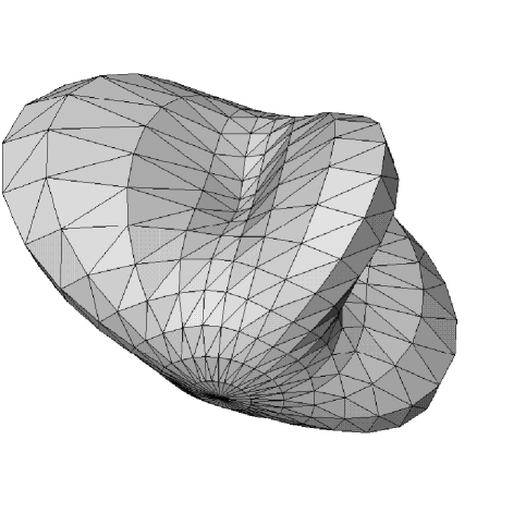
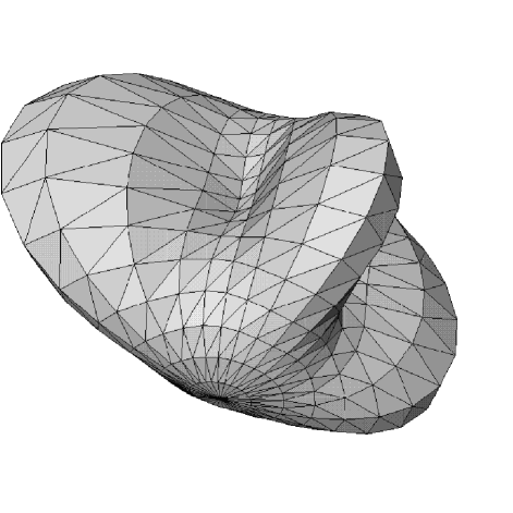
FIG. 1.: Embedding of a test surface defined by the spherical harmonic coefficients ($a_{00}=9$,$a_{22}=1$,$a_{44}=4$). The upper panel shows the original surface and the lower panel the resulting embedding.

Expansion	Original	Recovered
coefficient	value	value
$a_{00}$	9	$9+1.1\times 10^{-5}$
$a_{20}$	0	$-3.6\times 10^{-5}$
$a_{22}$	1	$1+4\times 10^{-6}$
$a_{40}$	0	$1.5\times 10^{-5}$
$a_{42}$	0	$-2.24\times 10^{-5}$
$a_{44}$	2	$2+1.9\times 10^{-5}$

TABLE I.: Comparison of the recovered expansion coefficients for the embedding of the test surface described in the text.

For this test we have used $100\times 100$ grid points to describe the surface. Since the surface is symmetric with respect to reflections on all three $(x,y,z)$ coordinate planes, we have considered only one octant, so the angular resolution was $\Delta\theta=\Delta\phi=\pi/200$. The recovered expansion coefficients are shown in Table I. The coefficients corresponding to the mapping of the angular coordinates, as well as the rest of the $Y_{lm}$ coefficients were either exactly zero because of the octant symmetry or had values smaller than $10^{-3}$.

Figure 2 shows a direct comparison of the metric components $g_{\theta\theta}$, $g_{\theta\phi}$ and $g_{\phi\phi}$ along the lines $\theta=\pi/4$ and $\phi=\pi/4$, i.e in the middle of the computational domain.

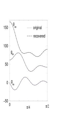
FIG. 2.: The difference in the metric components for the embedding of the test surface described in the text. On the left panel we show the line $\theta=\pi/4$ and on the right panel the line $\phi=\pi/4$.

The final value for the embedding function in this test was $F=1.6\times 10^{-5}$, but we have found that we can easily decrease this value by refining the numerical grid on the surface.

B An axisymmetric example: Rotating black holes

As already mentioned in section I, a well-known set of axisymmetric surfaces whose embeddings have been studied, first by Smarr [5], and also as a test case in [15], is that of the horizons of rotating black holes. In the static Kerr case, the metric of the horizon is given by

$$d\sigma^{2}=\rho^{2}\,d\theta^{2}+\frac{\sin^{2}\theta}{\rho^{2}}\,\left(r^{2}+a^{2}\right)\,d\phi^{2}\,,$$ (28)

with

$$\rho^{2}=r^{2}+a^{2}\cos^{2}\theta\,,\quad r=m+\sqrt{m^{2}-a^{2}}\,,$$ (29)

and where $m$ and $a$ are two parameters representing the mass of the black hole and its angular momentum respectively.

It is well known that the Kerr horizon is globally embeddable in flat space only for $a/m\leq\sqrt{3}/2$ [5]. Using our embedding code, we have been able to successfully recover these embeddings when they exist. As an example we show in Fig. 3 the embedding obtained for the last embeddable case $a/m=\sqrt{3}/2$. The solid line shows the embedding obtained with the axisymmetric algorithm described above, and the dotted line the one obtained with our minimization algorithm.

FIG. 3.: Embedding of a Kerr black hole with $a/m=\sqrt{3}/2$. The dotted line is the embedding we obtained using our minimization algorithm. The solid line is an embedding of the same surface computed with an axisymmetric algorithm.

When $a/m\geq\sqrt{3}/2$, a global embedding does not exist, and our method fails as expected. Figure 4 shows the result of an attempt to embed a Kerr black hole horizon in the case when $a/m=0.99$. The dotted line is the output of our minimization algorithm and the solid line is an embedding of the same surface made with an axisymmetric algorithm in the embeddable region, plus a flat top in the region where the embedding does not exist. The axisymmetric method is a local constructive method, and hence it is able to build the embedding surface from one point to the next where it exists (in this case starting from the equator). Since our method is global we get the embedding wrong everywhere. As currently implemented, our method will insist on trying to find a global embedding, and will settle on a shape that minimizes the function $F$. If the embedding does not exist, the minimum value of $F$ found will be clearly different from zero. This is easily seen by examining the residual function $F$ for the embeddings of the Kerr horizons. In Fig. 5 we show the value of the minimum of $F$ found with our algorithm, plotted against the total number of expansion coefficients, for the cases $a/m=\sqrt{3}/{2}$ (solid line) and $a/m=0.99$ (dotted line). One can see that for the non-embeddable case, $F$ stops decreasing at a value that is more than 2 orders of magnitude larger than the one we obtain when the embedding exists.

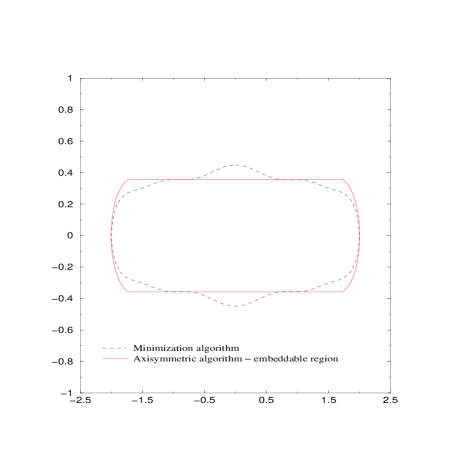
FIG. 4.: An attempt to embed a Kerr black hole horizon with $a/m=0.99$. The dotted line is the output of the minimization algorithm. The solid line is an embedding of the same surface made with an axisymmetric algorithm. The flat line on the top represents the region where an embedding in flat space does not exist.

FIG. 5.: The value of the embedding function $F$ versus the total number of coefficients for the two Kerr black holes discussed above. The triangles correspond to $a/m=0.99$ and the stars to $a/m=\sqrt{3}/{2}$.

Our code might be adjusted in the future for finding partial embeddings by reducing the integration domain in the definition of $F$, Eq. (26), to something smaller than the full sphere. This approach might lead to correct partial embeddings of surfaces that cannot be embedded globally. The disadvantage would be that one would have to guess the domain where the embedding exits before starting the computation.

C Black hole plus Brill wave

We now move to the case of numerically generated, distorted black holes. Schwarzschild black holes distorted by Brill waves [20] have been extensively studied in numerical relativity [21, 22, 23, 24]. The axisymmetric data sets used for numerical evolutions consist of a Schwarzschild black hole distorted by a toroidal, time-symmetric gravitational wave.

It is convenient to describe the metric of the black hole plus Brill wave spacetime in a spherical-polar like coordinate system $(\eta,\theta,\phi)$ were $\eta$ is a logarithmic radial coordinate defined by $\eta=\ln(2r/M)$ and $(\theta,\phi)$ are the standard angular coordinates. In these coordinates, the spatial metric has the form [6, 23]

$$dl^{2}=\Psi^{4}\left[e^{2q}\left(d\eta^{2}+d\theta^{2}\right)+r^{2}\sin^{2}\theta d\phi^{2}\right]\,,$$ (30)

where both $q$ and $\Psi$ are functions of $\eta$ and $\theta$ only. In order to satisfy the appropriate regularity and fall-off conditions, the function $q$ has been chosen in the following way

$$q(\eta,\theta)=a\sin^{n}\theta\,\left[e^{-\left(\frac{\eta+b}{\omega}\right)^{2}}+e^{-\left(\frac{\eta-b}{\omega}\right)^{2}}\right]\,,$$ (31)

with $n$ is an arbitrary even number larger than $0$. The parameter $a$ characterizes the amplitude of the Brill wave, while the parameters $b$ and $\omega$ characterize its radial location and width respectively. Having chosen the form of the function $q$, the hamiltonian constraint is solved numerically for the conformal factor $\Psi$. An isometry condition is imposed at a coordinate sphere to guarantee that the final spacetime will contain a black hole.

Notice that the metric (30) is the three-dimensional metric of space, and not the two-dimensional metric of the apparent horizons. The apparent horizons for these data sets have to be located numerically. Once these horizons are found, their two-dimensional metric can be computed from the three-dimensional metric given above, using the expressions given in (13).

The horizons from these axisymmetric black hole plus Brill wave data sets and their embeddings have been studied previously in [23] and we have been able to reproduce their results using our algorithm. An example of this can be seen in Fig. 6, where we show the embedding of the horizon of a black hole plus Brill wave data set corresponding to the parameters

$$a=1.0\,,\quad b=0.0\,,\quad w=1.0\,,\quad n=2\,.$$ (32)

FIG. 6.: Embedding of the apparent horizon of a black hole plus Brill wave data set corresponding to the parameters $(a=1.0,b=0.0,\omega=1.0,n=2)$. The dotted line is the embedding obtained with our minimization algorithm and the solid line the embedding of the same surface obtained by Anninos et al.

In the figure, the dotted line shows the embedding obtained with our minimization algorithm, and the solid line shows the embedding of the same surface obtained in [23]. Notice how the intrinsic geometry of the horizon is far from spherical.

D Application to Full 3D Spacetimes

Having tested our algorithm on both analytic and numerically generated axisymmetric black hole spacetimes, we now turn to the case of full 3D black hole spacetimes for which our method was developed.

The axisymmetric black hole plus Brill wave data sets from [23] have been generalized in [25] to full 3D by multiplying the Brill wave function $q$ by a factor that has azimuthal dependence to obtain

$$q(\eta,\theta,\phi) = a\sin^{n}\theta\,\left(1+c\,\cos^{2}\phi\right)$$ (34)

$$\left[e^{-\left(\frac{\eta+b}{\omega}\right)^{2})}+e^{-\left(\frac{\eta-b}{\omega}\right)^{2}}\right]\,,$$

were $c$ is an arbitrary parameter characterizing the non-axisymmetry of the Brill wave.

We have computed embeddings of the non axisymmetric apparent horizons obtained in this case. Here we will show examples of two such horizons. First we consider the embedding of the apparent horizon for the data set with parameters

$$a=0.3\,,\quad b=0.0\,,\quad\omega=1.0\,,\quad n=4\,,\quad c=0.4\,,$$ (35)

which corresponds to a relatively small non-axisymmetric distortion of the black hole. Figure 7 shows the embedding of the corresponding apparent horizon. Notice how the surface looks quite axisymmetric even though we have added a non-trivial non-axisymmetric contribution to the metric. It is clear that the non-axisymmetry of the metric components is to a large degree a coordinate effect. Numerical evolutions of such black holes do show radiation in non-axisymmetric modes of gravitational radiation. However the mass energy carried away by the non-axisymmetric modes is much smaller than the energy of the axisymmetric modes [26, 21]. This is consistent with our result showing that the horizon is almost axi-symmetric.

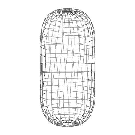
FIG. 7.: Embedding of the apparent horizon for the non axisymmetric black hole plus Brill wave data set corresponding to the parameters $(a=1.0,b=0.0,\omega=1.0,n=4,c=0.4)$. Although the metric has a non-trivial non-axisymmetric contribution, the surface looks quite axisymmetric.

Figure 8 shows a direct comparison of the different angular metric components on the apparent horizon and the resulting embedding, along the $\phi=\pi/4$ and $\theta=\pi/4$ lines. We can see how the fit is very good in both cases. Notice also how there is indeed some dependence of the metric components on $\phi$.

FIG. 8.: We show the angular metric components on the apparent horizon and on the resulting embedding for the black hole plus Brill wave data set corresponding to the parameters $(a=1.0,b=0.0,\omega=1.0,n=4,c=0.4)$. On the left panel we show the line $\theta=\pi/4$ and on the right panel the line $\phi=\pi/4$.

To check if our algorithm is converging to the correct embedding, we show in Fig. 9 the value of the embedding function $F$ at the minimum, in terms of the total number of expansion coefficients. We clearly see that the value of $F$ is converging exponentially to zero.

FIG. 9.: We show the value of the embedding function $F$ at the minimum in terms of the total number of expansion coefficients in a logarithmic scale for the black hole plus Brill wave data set corresponding to the parameters $(a=1.0,b=0.0,\omega=1.0,n=4,c=0.4)$.

As a second example, we now consider the embedding of the apparent horizon corresponding to the black hole plus Brill wave data set with parameters

$$a=0.3\,,\quad b=0.0\,,\quad\omega=1.0\,,\quad n=4\,,\quad c=1.9\,.$$ (36)

In this case, the non-axisymmetry is considerably larger, and one can see from Fig. 10 that the horizon is clearly not axisymmetric.

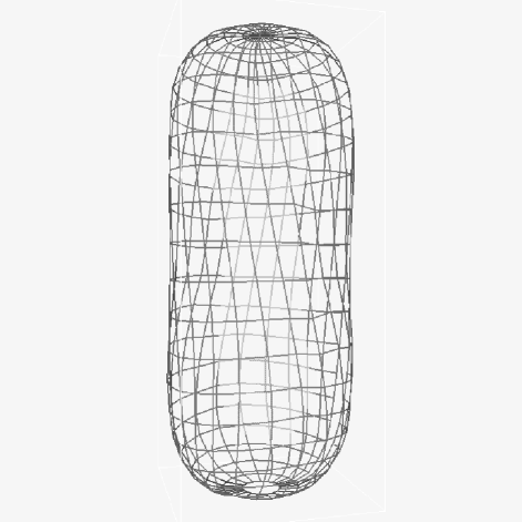
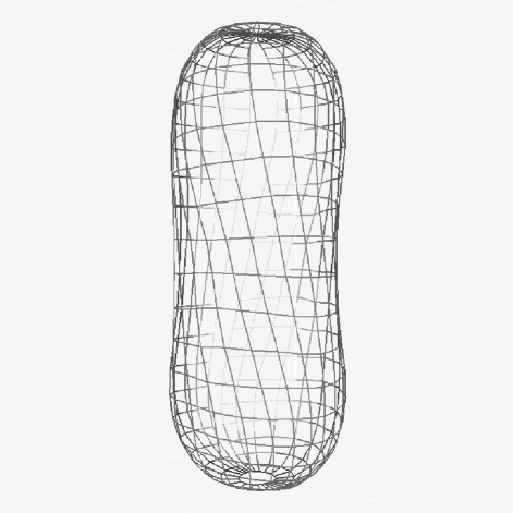
FIG. 10.: Two orientations of the embedding of the apparent horizon of a black hole perturbed by a Brill wave with a higher non-axisymmetry than in the previous example.

In Fig. 11 we show again a direct comparison of the angular metric components on the apparent horizon and the resulting embedding along the $\phi=\pi/4$ and $\theta=\pi/4$ lines. As before, the fit is very good.

FIG. 11.: The three independent components of the metric for the black hole plus Brill wave will a larger non-axisymmetric perturbation. On the left panel we show the line $\theta=\pi/4$ and on the right panel the line $\phi=\pi/4$.

Finally, in Fig. 12 we show again the value of the embedding function $F$ at the minimum in terms of the number of expansion coefficients. As before, the value of $F$ converges exponentially to zero, but the convergence is slower than in the previous example due to the higher degree of complexity of the surface.

FIG. 12.: The value of the embedding function $F$ at the minimum in terms of the total number of expansion coefficients on a logarithmic scale for the black hole plus Brill wave with a larger non-axisymmetric contribution.

IV Conclusions

We have implemented and tested a new algorithm for computing isometric embeddings of curved surfaces with spherical topology in flat space. We define a function on the space of surfaces that has a global minimum for the right embedding and we find this minimum using a standard minimization algorithm. In this paper we have discussed the method and its applications to black hole visualization in numerical relativity. The method has been tested both on simple test surfaces and on Kerr black hole horizons, and shown to correctly reproduce known results within specified tolerances. We have also used our method construct embeddings of non-axisymmetric, distorted black holes for the first time. We observed that the non-axisymmetry of the embedded surface is somehow smaller than one expects from just looking at the metric. This is consistent with the small amount of gravitational radiation emitted in non-axisymmetric modes during the numerical evolution of such systems [21, 26].

Our method is rather robust, and by construction produces smooth surfaces, therefore avoiding some of the problems of previous methods. One disadvantage of our method is that the expansion in spherical harmonics implies that it can only be used to embed ray-body surfaces (i.e. surfaces such that any ray coming from the origin intersects the surface at only one point), still we expect most black hole horizons to have this property. The main disadvantage, however, is that the method is very time consuming due to the fact that minimization algorithms in general are slow. Another problem is the fact that minimization algorithms can easily get trapped in local minima. In order to avoid this we have found it necessary to increase the number of coefficients one by one and to use at each step the result of the previous step as initial guess, adding to the total amount of time the algorithm needs to find the embedding. As presently implemented, it also cannot find partial embeddings when no global embeddings exist, but straightforward modifications to the algorithm should permit this in certain cases.

In the future, we will apply this method to study the dynamics of 3D black hole horizons as a tool to aid in understanding the physics of such systems. Although our method has been applied in this paper only to apparent horizons, it can clearly be applied to obtain embeddings of event horizons as well, once they have been located in numerical evolutions.

Our embedding algorithm has been implemented as a thorn in the Cactus code [27], and is available for the community upon request from the authors.

- [1] P. Anninos et al., Phys. Rev. D 50, 3801 (1994).
- [2] M. Berger and B. Gostiaux, Differential Geometry: Manifolds, Curves and Surfaces (Springer-Verlag, New York, 1998).
- [3] C. Misner, Phys. Rev. D 118, 1110 (1960).
- [4] J. D. Romano and R. H. Price, Class. Quantum GRav. 12, 875 (1995).
- [5] L. L. Smarr, Phys. Rev. D 7, 289 (1973).
- [6] D. Bernstein, Ph.D. thesis, University of Illinois Urbana-Champaign, 1993.
- [7] P. Anninos et al., IEEE Computer Graphics and Applications 13, 12 (1993).
- [8] P. Anninos et al., Phys. Rev. Lett. 74, 630 (1995).
- [9] P. Anninos et al., in The Seventh Marcel Grossmann Meeting: On Recent Developments in Theoretical and Experimental General Relativity, Gravitation, and Relativistic Field Theories, edited by R. T. Jantzen, G. M. Keiser, and R. Ruffini (World Scientific, Singapore, 1996), p. 648.
- [10] P. Anninos et al., Australian Journal of Physics 48, 1027 (1995).
- [11] A. Ashtekar, C. Beetle, and S. Fairhurst, Class. Quantum Grav. 16, L1 (1999).
- [12] A. Ashtekar, C. Beetle, and S. Fairhurst, Class. Quantum Grav. 17, 253 (2000).
- [13] A. Ashtekar et al., Phys. Rev. Lett. 85, 3564 (2000).
- [14] A. Ashtekar, C. Beetle, and J. Lewandowski, Phys. Rev. D 64, 044016 (2001).
- [15] H.-P. Nollert and H. Herold, in Relativity and Scientific Computing, edited by F. W. Hehl, R. A. Puntigam, and H. Ruder (Springer Verlag, Berlin, 1998), p. 330.
- [16] D. Bernstein et al., Phys. Rev. D 50, 5000 (1994).
- [17] J. Massó, E. Seidel, W.-M. Suen, and P. Walker, Phys. Rev. D 59, 064015 (1999).
- [18] M. R. Schroeder, Number Theory in Science and Communication (Springer-Verlag, Berlin, 1986).
- [19] W. H. Press, B. P. Flannery, S. A. Teukolsky, and W. T. Vetterling, Numerical Recipes (Cambridge University Press, Cambridge, England, 1986).
- [20] D. S. Brill, Ann. Phys. 7, 466 (1959).
- [21] G. Allen, K. Camarda, and E. Seidel, (1998), gr-qc/9806036, submitted to Phys. Rev. D.
- [22] K. Camarda and E. Seidel, Phys. Rev. D 57, R3204 (1998), gr-qc/9709075.
- [23] P. Anninos et al., Phys. Rev. D 52, 2059 (1995).
- [24] A. Abrahams et al., Phys. Rev. D 45, 3544 (1992).
- [25] K. Camarda, Ph.D. thesis, University of Illinois at Urbana-Champaign, Urbana, Illinois, 1998.
- [26] G. Allen, K. Camarda, and E. Seidel, (1998), gr-qc/9806014, submitted to Phys. Rev. D.
- [27] http://www.cactuscode.org.