Extended hierarchical search (EHS) algorithm for detection of gravitational waves from inspiraling compact binaries

Abstract

Pattern matching techniques like matched filtering will be used for online extraction of gravitational wave signals buried inside detector noise. This involves cross correlating the detector output with hundreds of thousands of templates spanning a multi-dimensional parameter space, which is very expensive computationally. A faster implementation algorithm was devised by Mohanty and Dhurandhar [1996] using a hierarchy of templates over the mass parameters, which speeded up the procedure by about 25 to 30 times. We show that a further reduction in computational cost is possible if we extend the hierarchy paradigm to an extra parameter, namely, the time of arrival of the signal. In the first stage, the chirp waveform is cut-off at a relatively low frequency allowing the data to be coarsely sampled leading to cost saving in performing the FFTs. This is possible because most of the signal power is at low frequencies, and therefore the advantage due to hierarchy over masses is not compromised. Results are obtained for spin-less templates up to the second post-Newtonian (2PN) order for a single detector with LIGO I noise power spectral density. We estimate that the gain in computational cost over a flat search is about 100.

1 Introduction

Massive compact binary systems consisting of neutron stars (up to a distance of 20 Mpc) or black-holes (up to 200 Mpc) ranging in masses from $\sim$ 0.5 $\mathrm{M}_{\odot}$ to $\sim$ 10.0 $\mathrm{M}_{\odot}$ are one of the most promising sources for large scale laser interferometric detectors for gravitational waves (GW). Few minutes before the final merger, the GW frequency of such sources will lie within the bandwidth of the detectors. The expected GW waveform of these sources is known adequately to allow pattern matching techniques like matched filtering to be used for signal extraction.

However matched filtering is computationally quite expensive, since hundreds of thousands of templates must be used to search the multidimensional parameter space. The hierarchical search algorithm of Mohanty and Dhurandhar [1] which employed a hierarchy of templates over the mass parameters achieved a significant improvement in cutting down the cost by a factor between 25 and 30. In this paper we explore the possibility of extending the hierarchical paradigm to an extra dimension - the time of arrival of the signal. This is achieved by using the idea of decimating the signal in time (proposed before in [2] but not worked out in detail). This reduces the computational cost by about a factor of 100 over the 1-step search described in Section 2 for a single detector with LIGO I noise power spectral density.

2 The 1-step search

In the stationary phase approximation, the Fourier transform $\tilde{h}(f)$ of the spin-less restricted second order post-Newtonian (2PN) waveform up to a constant factor $\mathcal{N}$, is given by

$$\tilde{h}(f)=\mathcal{N}f^{-7/6}\exp i\left[-\frac{\pi}{4}-\Phi_{0}+\Psi(f;M,\eta)\right],$$ (1)

where $M$ is the total mass of the binary system, $\eta$ is the ratio of the reduced mass to the total mass, $\Phi_{0}$ is the initial phase at some fiducial frequency $f_{a}$, and $f$ is the frequency. $\mathcal{N}$ depends on [3] the masses, the distance to the binaries and $f_{a}$.

The function $\Psi(f;M,\eta)$ describes the phase evolution of the inspiral waveform and is given by,

$$\Psi(f;M,\eta)=2\pi ft_{0}+\frac{3}{128\eta}\left[(\pi Mf)^{-5/3}+\left(\frac{3715}{756}+\frac{55}{9}\right)(\pi Mf)^{-1}\right.$$

$$\left.-16\pi(\pi Mf)^{-2/3}+\left(\frac{15293365}{508032}+\frac{27145}{504}\eta+\frac{3085}{72}\eta^{2}\right)(\pi Mf)^{-1/3}\right].$$ (2)

The kinematical parameters $(t_{0},\Phi_{0})$ do not determine the shape of the waveform and can be treated very simply in the matched filtering procedure [4]. In what follows, the parameter space will explicitly refer to the space of dynamical parameters that determine the phase, and thus the shape of the waveform . For the 2PN case, it is the two dimensional space described by $M\,\mathrm{and}\,\eta$. In order to facilitate the analysis one chooses a new set of parameters $\tau_{0}$ and $\tau_{3}$ in which the metric defined over the parameter space [5] is approximately constant. They are related to $M$ and $\eta$ by

$$\tau_{0}=\frac{5}{256\,\eta f_{a}}\left(\pi Mf_{a}\right)^{-5/3},\,\,\,\tau_{3}=\frac{1}{8\eta f_{a}}\left(\pi Mf_{a}\right)^{-2/3}.$$ (3)

In these new co-ordinates the parameter space is wedge shaped as shown in the left panel of Figure 1.

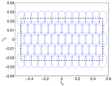
Figure 1: Left panel shows the parameter space for 2PN waveforms in $(\tau_{0},\tau_{3})$ space for binary masses in the range $1.0\,\mathrm{M}_{\odot}\leq m_{1},m_{2}\leq 30.0\,\mathrm{M}_{\odot}$. The fiducial frequency is set to $f_{a}=40.0$ Hz for this figure and the area is $8.5\,\mathrm{sec}^{2}$. Shown on the right panel is a schematic of discrete template placement using hexagonal closed packing (hcp). The spacing between neighboring templates is very small compared to the total area, and thus we can extend the method to the whole parameter space.

A straight forward implementation of matched filtering involves constructing a discrete lattice of normalized templates over the parameter space and computing correlations with the detector output. The bandwidth over which the correlations are computed in the frequency space, is taken from the seismic lower cutoff frequency $f_{s}$ to a upper cutoff frequency $f_{c}$. For the LIGO laboratory accepted noise PSD [6], we set $f_{s}=30\,\mathrm{Hz}$ and $f_{u}=800\,\mathrm{Hz}$. The maximum of the correlation output is compared with the threshold $\eta_{2}$ (we put the subscript ‘2’ because $\eta_{2}$ will be used as the second stage threshold in the hierarchical scheme described later) which depends on a pre-decided false alarm rate usually set at one per year. The false alarm rate we assume here is for one detector only. If the data is sampled at $2048\,\mathrm{Hz}$, the noise assumed to be a Gaussian stationary process and the number of templates $\sim 10^{4}$ then the threshold $\eta_{2}\simeq 8.2$. Detection is announced if the maximum correlation exceeds this threshold.

The degree of discretization of templates is governed by a maximum mismatch between the signal and the filter, which is taken to be $3\%$ (corresponding to a maximum loss of event rate of $10\%$). The mismatch in terms of the parameters $(\tau_{0},\tau_{3})$ is encoded in the ambiguity function $\mathcal{H}(\Delta\tau_{0},\Delta\tau_{3})$. Actually $\mathcal{H}$ also depends weakly on the position $(\tau_{0},\tau_{3})$, but we ignore its effect in the present analysis. We use the most efficient hexagonal closed packing (hcp) tiling for placing the templates as shown in Figure 1 (right panel), with a packing fraction of $83\%$. This leads to 17000 templates for LIGO I noise PSD and for a mass range of $1.0\,-\,30.0\,\mathrm{M}_{\odot}$. Sampling at $2048\,\mathrm{Hz}$ with a data train $512$ sec long to allow for $75\%$ padding, the number of points in the data train is $2^{20}$. The online speed required to cover the cost of FFTs amounts to 2.54 G-Flops using this 1-step implementation of matched filtering. The required speed rises to about 15 G-Flops if the minimum mass of the mass range is reduced to $0.5\mathrm{M}_{\odot}$ and to about 150 G-Flop when the minimum mass is $0.2\,\mathrm{M}_{\odot}$.

3 Extended hierarchical search

The hierarchical scheme as given in [1] involves parsing the data through two template banks instead of one. The basic idea is to use a coarse bank of templates in the first stage along with a lower threshold. This allows the parameter space to be scanned with less number of templates. However the lower threshold leads to a large number of false alarms which must be then followed up with a fine bank (maximum mismatch $3\%$) search.

3.1 Methodology

The above idea can be extended to include the time of arrival of the signal - by cutting off the chirp at a lower frequency $f_{\mathrm{cutoff}}$ and re-sampling it at a lower Nyquist rate in the trigger phase of a two step implementation of matched filtering. This is possible because the inspiral signal contains most of the signal power at lower frequencies ( the power spectrum scales as $\left|\tilde{h}(f)\right|^{2}\propto f^{-7/3}$) and thus we do not lose much of the SNR. The fractional SNR that can be recovered in this case is given by $\mathrm{SNR}(f_{\mathrm{cutoff}})=I(f_{\mathrm{cutoff}})\left/I(f_{u})\right.$, where

$$I(f_{\mathrm{cutoff}})=2\int_{f_{s}}^{f_{\mathrm{cutoff}}}\frac{df}{f^{7/3}\,S_{h}(f)}\,,\,\,\,\,\,f_{s}<f_{\mathrm{cutoff}}\leq f_{u}\,.$$ (4)

In the left panel of Figure 2 we have plotted the relative SNR as a function of the cutoff frequency. As can be clearly seen, a significant fraction of the signal power can be recovered from a relatively small value of $f_{\mathrm{cutoff}}$. Specifically, for $f_{\mathrm{cutoff}}=256\,\mathrm{Hz}$, almost $92\%$ of the SNR can be recovered. Since not too much of the SNR is lost, the hierarchy over the masses [7] is not compromised too severely.

The most obvious advantage of lowering the Nyquist rate in the first stage is that we have fewer points to contend with in computing the FFTs (the cost of FFTs scale as $N\log_{2}N$), leading to reduction in cost. For example, $f_{\mathrm{cutoff}}=256\,\mathrm{Hz}$ reduces the sampling rate to a quarter, reducing the cost of FFTs by almost the same factor. Secondly, the ambiguity function becomes wider thereby reducing the number of templates used in the first stage and reducing the cost.

The first stage threshold $\eta_{1}$ is set by striking a balance between the two opposing effects; (i) $\eta_{1}$ must be low enough to allow coarsest possible placement of trigger stage templates so that the first stage computational cost is minimized, (ii) $\eta_{1}$ must be high enough to reduce the number of false crossings, so that the second stage cost is reduced.

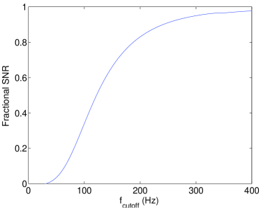
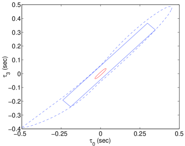
Figure 2: The left panel shows the fraction of signal to noise ratio (SNR) extracted as a function of the cut off frequency $f_{\mathrm{cutoff}}$. The SNR is normalized to 1 for $f_{\mathrm{cutoff}}=f_{u}\,\mathrm{Hz}$. The right panel shows the $\mathcal{H}(\Delta\tau_{0},\Delta\tau_{3})=0.80$ contours along with the largest inscribed rectangle used in the trigger stage of EHS algorithm for $f_{\mathrm{cutoff}}=256\,\mathrm{Hz}$. The ellipse inside the rectangle is that used by 1-step search to tile the space and is given for comparison of the areas.

By choosing $\eta_{1}$ optimally, the total computational cost arising from both the stages is minimized.

3.2 Computational cost of the EHS

We consider data trains of length $512\,\mathrm{sec}$ which accommodate chirps of maximum length $95\,\mathrm{sec}$ with sufficient padding corresponding to minimum mass limit of $1.0\,\mathrm{M}_{\odot}$. We consider first and second stage sampling frequencies of $512\,\mathrm{Hz}$ and $2048\,\mathrm{Hz}$ respectively. The cutoff frequency in the first stage is set at $f_{\mathrm{cutoff}}=256\,\mathrm{Hz}$. Thus the data points to be processed are $2^{18}$ and $2^{20}$ for the coarse and fine banks respectively. The second stage threshold is set at $\eta_{2}\simeq 8.2$ as before (see Section 2) for a false alarm rate of one per year. The signals of minimal strength that can be observed, assuming a minimum detection probability of $95\%$ and $3\%$ mismatch between templates turns out to be $9.17$. The first stage $\mathrm{SNR}$ for the above mentioned cutoff can be calculated to be $92\%$ of 9.17 which is 8.44. It is found that the total cost is minimized for $\eta_{1}\approx 6$. Again, assuming a minimum detection probability of $95\%$ in the first stage itself, the ambiguity function can be allowed to drop to $6.75$ which is about $80\%$ of its maximum value. This large drop allows for very big tiles as shown in the right panel of Figure 2. However, the awkward shape of these tiles makes tiling the parameter space a difficult proposition. We surmount this problem by cutting out the largest inscribed rectangle as shown in the same figure which has an area of $0.05\,\mathrm{sec}^{2}$. This is $\sim 50$ times larger than the area of second stage tiles. Combining the first and second stage costs, the required online speed is then estimated at 19.54 M-Flops, giving a gain factor of about 130 over the one step search.

4 Discussion

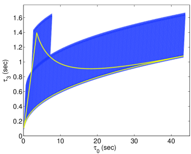
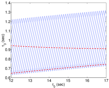
Figure 3: The left panel shows a possible schematic lay-out of first stage templates for implementing the EHS algorithm. Note that far too many templates have to be used in the first stage to cover the parameter space, due to inefficient tiling. The effect is most severe towards the tapering low mass end of the parameter space. The right panel shows the details of first stage template placement at a higher resolution. The dashed line in this figure is the parameter space boundary.

We have shown that a three dimensional hierarchical search for gravitational waves emitted by inspiraling compact binaries is a highly promising proposition. We have obtained a computational cost reduction factor of about 130 for an ideal search, when the parameter space can be optimally tiled by the first stage template rectangles. However due to boundary effects this factor can be drastically reduced. As can be seen in Figure 3, the parameter space tapers towards the low mass end where the tiling becomes inefficient. Most of the tiles go ‘out’ of the deemed parameter space. It is estimated that this can cut down the above mentioned gain factor by about $50\%$. These effects become less pronounced when the lower mass limit of the mass range is reduced. We expect to recover the gain factor to about 100, if the lower mass limit is reduced to less than $0.5\,\mathrm{M}_{\odot}$.

The second important effect, affecting the gain factor, will come from the rotation of the first and second stage tiles and also the differential rotation between them. These effects have still to be taken into account and will be the thrust of our future investigations. However, we do not expect this effect to alter the gain factor very much.

References

- [1] S.D. Mohanty and S.V. Dhurandhar, Phys. Rev. D 54, 7108 (1996).
- [2] T. Tanaka and T. Tagoshi, Phys. Rev. D 62, 082001 (2000).
- [3] S.V. Dhurandhar and B.S. Sathyaprakash, Phys. Rev. D 49, 1707 (1994).
- [4] B.S. Sathyaprakash and S.V. Dhurandhar, Phys. Rev. D 44, 3819 (1991).
- [5] B.J. Owen, Phys. Rev. D 57, 6749 (1996).
-
[6]
Plots and data files of LIGO I noise curve is maintained by J.K. Blackburn
and is available at the URL
www.ligo.caltech.edu/~kent/ASIS_NM/initial.html - [7] S.D. Mohanty, Phys. Rev. D 57, 630 (1998).