Dynamical instability of new-born neutron stars as sources of gravitational radiation

Abstract

The dynamical instability of new-born neutron stars is studied by evolving the linearized hydrodynamical equations. The neutron stars considered in this paper are those produced by the accretion induced collapse of rigidly rotating white dwarfs. A dynamical bar-mode ($m=2$) instability is observed when the ratio of rotational kinetic energy to gravitational potential energy $\beta$ of the neutron star is greater than the critical value $\beta_{d}\approx 0.25$. This bar-mode instability leads to the emission of gravitational radiation that could be detected by gravitational wave detectors. However, these sources are unlikely to be detected by LIGO II interferometers if the event rate is less than $10^{-6}$ per year per galaxy. Nevertheless, if a significant fraction of the pre-supernova cores are rapidly rotating, there would be a substantial number of neutron stars produced by the core collapse undergoing bar-mode instability. This would greatly increase the chance of detecting the gravitational radiation.

PACS: 04.30.Db, 95.30.Sf, 97.60.Jd

I Introduction

Neutron stars are believed to form from the core collapse of massive stars and the accretion induced collapse of massive white dwarfs. If the stellar core or white dwarf is rotating, conservation of angular momentum implies that the resulting neutron star must rotate very rapidly. It has been suggested [1] that such a rapidly rotating star may develop a non-axisymmetric dynamical instability, emitting a substantial amount of gravitational radiation which might be detectable by gravitational wave observatories such as LIGO, VIRGO, GEO and TAMA.

Rotational instabilities arise from non-axisymmetric perturbations having angular dependence $e^{im\varphi}$, where $\varphi$ is the azimuthal angle. The $m=2$ mode is called the bar mode, which is usually the strongest mode for stars undergoing instabilities. There are two types of instabilities. A dynamical instability is driven by hydrodynamics and gravity, and it develops on a dynamical timescale, i.e. the timescale for a sound wave to travel across the star. A secular instability, on the other hand, is driven by viscosity or gravitational radiation reaction, and its growth time is determined by the relevant dissipative timescale. These secular timescales are usually much longer than the dynamical timescale of the system.

In this paper, we focus on the dynamical instabilities resulting from the new-born neutron stars formed from accretion induced collapse (AIC) of white dwarfs. These instabilities occur only for rapidly rotating stars. A useful parameter to characterize the rotation of a star is $\beta=T/|W|$, where $T$ and $W$ are the rotational kinetic energy and gravitational potential energy respectively. It is well-known that there is a critical value $\beta_{d}$ so that a star will be dynamically unstable if its $\beta>\beta_{d}$. For a uniform density and rigidly rotating star, the Maclaurin spheroid, the critical value is determined to be $\beta_{d}\approx 0.27$ [2]. Numerous numerical simulations using Newtonian gravity show that $\beta_{d}$ remains roughly the same for differentially rotating polytropes having the same specific angular momentum distribution as the Maclaurin spheroids [3, 4, 5, 6, 7, 8, 9, 10, 11]. However, $\beta_{d}$ can take values between 0.14 to 0.27 for other angular momentum distributions [12, 9, 13] (the lower limit $\beta_{d}=0.14$ is observed only for a star having a toroidal density distribution, i.e. the maximum density occurs off the center [13]). Numerical simulations using full general relativity and post-Newtonian approximations suggest that relativistic corrections to Newtonian gravity cause $\beta_{d}$ to decrease slightly [14, 15, 16].

Most of the stability analyses to date have been carried out by assuming that the star rotates with an ad hoc rotation law or using simplified equations of state. The results of these analyses might not be applicable to the new-born neutron stars resulting from AIC. Recently, Fryer, Holz and Hughes [17] carried out an AIC simulation using a realistic rotation law and a realistic equation of state. Their pre-collapse white dwarf has an angular momentum $J=10^{49}~{}\rm{g}~{}\rm{cm}^{2}~{}\rm{s}^{-1}$. After the collapse, the neutron star has $\beta$ less than 0.06, which is too small for the star to be dynamically unstable. However, they point out that if the pre-collapse white dwarf spins faster, the resulting neutron star could have high enough $\beta$ to trigger a dynamical instability. They also point out that a pre-collapse white dwarf could easily be spun up to rapid rotation by accretion. The spin of an accreting white dwarf before collapse depends on its initial mass, its magnetic field strength and the accretion rate, etc. [18].

Liu and Lindblom [19] (hereafter Paper I) in a recent paper construct equilibrium models of new-born neutron stars resulting from AIC based on conservation of specific angular momentum. Their results show that if the pre-collapse white dwarfs are rapidly rotating, the resulting neutron stars could have $\beta$ as large as 0.26, which is slightly smaller than the critical value $\beta_{d}$ for Maclaurin spheroids. However, the specific angular momentum distributions of those neutron stars are very different from that of Maclaurin spheroids. So there is no reason to believe that the traditional value $\beta_{d}=0.27$ can be applied to those models.

The purpose of this paper is first to determine the critical value $\beta_{d}$ for the new-born neutron stars resulting from AIC, and then estimate the signal to noise ratio and detectability of the gravitational waves emitted as a result of the instability. We do not intend to provide an accurate number for the signal to noise ratio, which requires a detailed non-linear evolution of the dynamical instability. Instead, we use Newtonian gravitation theory to compute the structure of new-born neutron stars. Then we evolve the linearized Newtonian hydrodynamical equations to study the star’s stability and determine the critical value $\beta_{d}$. Relativistic effects are expected to give a correction of order $(v/c)^{2}$, which is about 8% for the rapidly rotating neutron stars studied in this paper. Here $v$ is a typical sound speed inside the star and $c$ is the speed of light.

This paper is organized as follows. In Sec. II, we apply the method described in Paper I to construct a number of equilibrium neutron star models with different values of $\beta$. In Sec. III, we study the stability of these models by adding small density and velocity perturbations to the equilibrium models. Then we evolve the perturbations by solving linearized hydrodynamical equations proposed by Toman et al [29]. From the simulations, we can find out whether the star is stable, and determine the critical value $\beta_{d}$. In Sec. IV, we estimate the strength and signal to noise ratio of the gravitational waves emitted by this instability. In Sec. V, we estimate the effects of a magnetic field on the stability results. Finally, we summarize and discuss our results in Sec. VI.

II Equilibrium Models

In this section, we describe briefly how we construct new-born neutron star models from the pre-collapse white dwarfs. A more detailed description is given in Paper I.

A Pre-collapse white dwarf models

We consider two types of pre-collapse white dwarfs: those made of carbon-oxygen (C-O) and those made of oxygen-neon-magnesium (O-Ne-Mg). The collapse of a massive C-O white dwarf is triggered by the explosive carbon burning near the center of the star [20, 21]. The central density of the pre-collapse C-O white dwarf must be in the range $6\times 10^{9}~{}\rm{g}~{}\rm{cm}^{-3}\stackrel{{\scriptstyle<}}{{{}_{\sim}}}\rho_{c}\stackrel{{\scriptstyle<}}{{{}_{\sim}}}10^{10}~{}\rm{g}~{}\rm{cm}^{-3}$ in order for the collapse to result in a neutron star, rather than exploding as a Type Ia supernova [22]. The collapse of a massive O-Ne-Mg white dwarf, on the other hand, is triggered by electron captures by ${}^{24}\rm{Mg}$ and ${}^{20}\rm{Ne}$ when the central density reaches $4\times 10^{9}~{}\rm{g}~{}\rm{cm}^{-3}$ [20, 21].

We construct three sequences of pre-collapse white dwarfs, with models in each sequence having different amounts of rotation. Sequences I and II correspond to C-O white dwarfs with central densities $\rho_{c}=10^{10}~{}\rm{g}~{}\rm{cm}^{-3}$ and $\rho_{c}=6\times 10^{9}~{}\rm{g}~{}\rm{cm}^{-3}$ respectively. Sequence III is for O-Ne-Mg white dwarfs with $\rho_{c}=4\times 10^{9}~{}\rm{g}~{}\rm{cm}^{-3}$. All white dwarfs are assumed to rotate rigidly, because the timescale for a magnetic field to suppress differential rotation is much shorter than the accretion timescale (see Sec. VI).

The pre-collapse white dwarfs constructed in this section are described by the equation of state (EOS) of a zero-temperature ideal degenerate electron gas with electrostatic corrections derived by Salpeter [23]. At high density, the pressure is dominated by the ideal degenerate Fermi gas with electron fraction $Z/A=0.5$ that is suitable for both C-O and O-Ne-Mg white dwarfs. Electrostatic corrections, which depend on the white dwarf composition through the atomic number $Z$, contribute only a few percent to the EOS for the high density white dwarfs considered here.

Equilibrium models are computed by Hachisu’s self-consistent field method [24], which is an iteration scheme based on the integrated Euler equation for hydrostatic equilibrium:

$$h+\Phi-\frac{\varpi^{2}}{2}\Omega^{2}=C\ ,$$ (1)

where $\Omega$ is the rotational angular frequency of the star; $C$ is a constant; $\varpi$ is the radius from the rotation axis; $h$ is the specific enthalpy, which is related to the density $\rho$ and pressure $P$ by

$$h=\int_{0}^{P}\frac{dP}{\rho}\ .$$ (2)

The gravitational potential $\Phi$ satisfies the Poisson equation

$$\nabla^{2}\Phi=4\pi G\rho\ ,$$ (3)

where $G$ is the gravitational constant. The self-consistent field method determines the structure of the star for fixed values of two adjustable parameters. In Ref. [24], the maximum density and axis ratio (the ratio of polar to equatorial radii) are the chosen parameters. However, it is more convenient to choose the central density $\rho_{c}$ and equatorial radius $R_{e}$ as the two parameters for the models studied here.

TABLE I.: Properties of pre-collapse white dwarfs. Here $\Omega$ is the rotational angular frequency; $\Omega_{m}$ is the maximum rotational angular frequency of the white dwarf in the sequence without mass-shedding; $R_{e}$, $R_{p}$, $M$, $J$ and $\beta$ are respectively the equatorial radius, polar radius, mass, angular momentum and the ratio of rotational kinetic to gravitational potential energies.

Sequence I: C-O white dwarfs with $\rho_{c}=10^{10}~{}\rm{g}~{}\rm{cm}^{-3}$

$\Omega/\Omega_{m}$	$R_{e}$	$R_{e}/R_{p}$	$M/M_{\odot}$	$J$	$\beta$
	(km)			($\rm{g}~{}\rm{cm}^{2}~{}\rm{s}^{-1}$)
0.20	1310	1.01	1.40	$5.14\times 10^{48}$	$5.36\times 10^{-4}$
0.65	1400	1.09	1.42	$1.81\times 10^{49}$	$6.08\times 10^{-3}$
0.84	1500	1.19	1.44	$2.43\times 10^{49}$	$1.03\times 10^{-2}$
0.93	1600	1.27	1.46	$2.80\times 10^{49}$	$1.30\times 10^{-2}$
1.00	1895	1.52	1.47	$3.12\times 10^{49}$	$1.55\times 10^{-2}$

Sequence II: C-O white dwarfs with $\rho_{c}=6\times 10^{10}~{}\rm{g}~{}\rm{cm}^{-3}$

$\Omega/\Omega_{m}$	$R_{e}$	$R_{e}/R_{p}$	$M/M_{\odot}$	$J$	$\beta$
	(km)			($\rm{g}~{}\rm{cm}^{2}~{}\rm{s}^{-1}$)
0.23	1517	1.01	1.39	$3.31\times 10^{48}$	$7.73\times 10^{-4}$
0.64	1610	1.09	1.42	$1.95\times 10^{49}$	$6.11\times 10^{-3}$
0.84	1740	1.19	1.44	$2.75\times 10^{49}$	$1.12\times 10^{-2}$
0.93	1847	1.28	1.45	$3.13\times 10^{49}$	$1.39\times 10^{-2}$
1.00	2189	1.52	1.46	$3.51\times 10^{49}$	$1.66\times 10^{-2}$

Sequence III: O-Ne-Mg white dwarfs with $\rho_{c}=4\times 10^{10}~{}\rm{g}~{}\rm{cm}^{-3}$

$\Omega/\Omega_{m}$	$R_{e}$	$R_{e}/R_{p}$	$M/M_{\odot}$	$J$	$\beta$
	(km)			($\rm{g}~{}\rm{cm}^{2}~{}\rm{s}^{-1}$)
0.23	1692	1.01	1.38	$7.01\times 10^{48}$	$7.90\times 10^{-4}$
0.62	1791	1.09	1.40	$2.05\times 10^{49}$	$6.23\times 10^{-3}$
0.86	1956	1.20	1.42	$3.03\times 10^{49}$	$1.23\times 10^{-2}$
0.96	2156	1.34	1.44	$3.59\times 10^{49}$	$1.62\times 10^{-2}$
1.00	2441	1.52	1.45	$3.80\times 10^{49}$	$1.77\times 10^{-2}$

The accuracy of the equilibrium models can be measured by the quantity

$$\epsilon=\left|\frac{2T+W+3\Pi}{W}\right|\ ,$$ (4)

which should be equal to zero according to the Virial theorem (see e.g. [25]). Here $T$ is the rotational kinetic energy; $W$ is the gravitational potential energy and $\Pi=\int Pd^{3}x$. The values of $\epsilon$ are of order $10^{-7}$ for all the pre-collapse white dwarf models calculated in this section. Table I shows some properties of several pre-collapse white dwarfs in the three sequences. Each sequence terminates when the rotational angular frequency $\Omega$ of the white dwarf reaches a critical value $\Omega_{m}$ so that the mass-shedding occurs on the equatorial surface of the star. The values of $\Omega_{m}$ are $5.37~{}\rm{rad}~{}\rm{s}^{-1}$ for Sequence I, $4.32~{}\rm{rad}~{}\rm{s}^{-1}$ for Sequence II, and $3.65~{}\rm{rad}~{}\rm{s}^{-1}$ for Sequence III.

FIG. 1.: The normalized specific angular momentum $j$ as a function of the cylindrical mass fraction $m_{\varpi}$ for the white dwarf model in sequence III with $\Omega/\Omega_{m}=0.964$.

Fig. 1 shows the normalized specific angular momentum

$$j=\frac{M}{J}\Omega\varpi^{2}$$ (5)

as a function of the cylindrical mass fraction

$$m_{\varpi}=\frac{2\pi}{M}\int_{0}^{\varpi}d\varpi^{\prime}\,\varpi^{\prime}\int_{-\infty}^{\infty}dz^{\prime}\,\rho(\varpi^{\prime},z^{\prime})$$ (6)

for a typical pre-collapse model. Here $M$ and $J$ are the total mass and angular momentum of the star respectively. The specific angular momentum defined in Eq. (5) is normalized so that $\int_{0}^{1}j(m_{\varpi})\,dm_{\varpi}=1$. The curves for other models are similar. The spike near $m_{\varpi}=1$ is due to the high degree of central condensation of the white dwarf density (Paper I).

B Collapsed objects

The gravitational collapse of a massive white dwarf is halted when the core density reaches nuclear density. The core bounces back and settles down into hydrodynamical equilibrium in a few milliseconds. A hot ($T\stackrel{{\scriptstyle>}}{{{}_{\sim}}}20~{}\rm{Mev}$) and lepton-rich proto-neutron star is formed. After about 20 s, neutrinos carry away most of the energy and the star cools down to a cold neutron star. The hot proto-neutron stars are less compact and have $\beta$ smaller than 0.14 (Paper I). They are thus expected to be dynamically stable. Hence in this paper, we focus on the stability of the cold neutron stars shortly after the cooling.

We assume that (1) the neutron stars are axisymmetric and are in rotational equilibrium with no meridional circulation; (2) viscosity can be neglected; (3) no material is ejected during the collapse. Under these assumptions, it is easy to prove that (see e.g. [19, 25]) the specific angular momentum $j$ of the collapsed star as a function of cylindrical mass fraction $m_{\varpi}$ is the same as the pre-collapse white dwarf. Hence the structure of the new-born neutron stars can be constructed by computing models with the same masses, angular momentum and $j(m_{\varpi})$-distributions as the pre-collapse white dwarfs.

We adopt the Bethe-Johnson EOS [26] for densities above $10^{14}~{}\rm{g}~{}\rm{cm}^{-3}$, and BBP EOS [27] for densities in the range $10^{11}-10^{14}~{}\rm{g}~{}\rm{cm}^{-3}$. The EOS for densities below $10^{11}~{}\rm{g}~{}\rm{cm}^{-3}$ is joined by that of the pre-collapse white dwarfs.

We construct the equilibrium models by the numerical method proposed by Smith and Centrella [28], which is a modified version of Hachisu’s self-consistent field method so that $j(m_{\varpi})$ can be specified. The iteration scheme is based on the integrated Euler equation (1) written in the form

$$h=C-\Phi+\left(\frac{J}{M}\right)^{2}\int_{0}^{\varpi}d\varpi^{\prime}\,\frac{j^{2}(m_{\varpi^{\prime}})}{\varpi^{\prime 3}}\ ,$$ (7)

where $J$ and $M$ are the total angular momentum and mass of the star respectively. As before, two parameters have to be fixed in the iteration procedure. We choose to fix the central density $\rho_{c}$ and equatorial radius $R_{e}$. Since the correct $\rho_{c}$ and $R_{e}$ are not known beforehand, we have to vary these two quantities until the equilibrium model has the same $J$ and $M$ as the pre-collapse white dwarf.

The standard iteration algorithm described in Refs. [24] and [28] fails to converge when the star becomes very flattened. This problem is fixed by a modified scheme proposed by Pickett, Durisen and Davis [9], in which only a fraction of the revised density (or enthalpy) $\rho_{i+1}$, i.e. $\rho^{\prime}_{i+1}=(1-\zeta)\rho_{i+1}+\zeta\rho_{i}$, is used for the next iteration. Here $\zeta<1$ is a parameter controlling the change of density. A value of $\zeta>0.95$ has to be used for very flattened configurations, and it takes 100-200 iterations for the density and enthalpy distributions to converge.

Paper I mentions another numerical difficulty which has to do with the spike of the $j(m_{\varpi})$ curve near $m_{\varpi}=1$. The authors of Paper I have to truncate a small portion of the $j(m_{\varpi})$ curve in order to make the iteration converge. They also demonstrate that this truncation does not affect the inner structure of the star. It turns out that, for reasons still to be understood, the numerical instability associated with the $j(m_{\varpi})$ curve only occurs for the most rapidly rotating models (i.e. those models where the pre-collapse white dwarfs have $\Omega/\Omega_{m}=1$). Hence, the truncation is not necessary for all the other cases.

FIG. 2.: The values of $\beta$ of the resulting neutron stars as a function of $\Omega/\Omega_{m}$ of the pre-collapse white dwarfs.

As in the case of pre-collapse white dwarfs, we measure the accuracy of the equilibrium models by the quantity $\epsilon$ defined in Eq. (4). The models computed in this subsection have $\epsilon$ ranges from about $10^{-6}$ (for slowly rotating stars) to $10^{-4}$ (for rapidly rotating stars). We construct a number of neutron star models resulting from the collapse of the three sequences of pre-collapse white dwarfs in the previous subsection. The ratio of rotational kinetic energy to gravitational potential energy, $\beta$, of the neutron stars is plotted in Fig. 2 as a function of $\Omega/\Omega_{m}$ of the pre-collapse white dwarf. The values of $\beta$ for all the neutron star models are smaller than 0.27, the critical value of $\beta$ for the dynamical instability of rigidly rotating Maclaurin spheroids.

FIG. 3.: Meridional density contours of the neutron star resulting from the AIC of a rigidly rotating O-Ne-Mg white dwarf with $\Omega/\Omega_{m}=0.964$. This neutron star has $\beta=0.255$. The contours in the upper graph denote, from inward to outward, $\rho/\rho_{c}=10^{-4},\ 10^{-5},\ 10^{-6},\ 10^{-7},\ 10^{-8},\ 10^{-9}\ \rm{and}\ 0$. The contours in the lower graph denote, from inward to outward, $\rho/\rho_{c}=0.8,\ 0.6,\ 0.4,\ 0.2,\ 0.1,\ 10^{-2},\ 10^{-3}\ \rm{and}\ 10^{-4}$. The central density of the star is $\rho_{c}=3.3\times 10^{14}~{}\rm{g}~{}\rm{cm}^{-3}$.

The structure of the neutron stars with $\beta\stackrel{{\scriptstyle>}}{{{}_{\sim}}}0.1$ are all similar: they contain a high-density central core of size about 20 km, surrounded by a low-density torus-like envelope. The size of the envelope depends on the amount of rotation of the star, which can be measured by $\beta$. The size ranges from 100 km (for $\beta\sim 0.1$) to over 500 km (for $\beta\stackrel{{\scriptstyle>}}{{{}_{\sim}}}0.2$). Figure 3 shows the density contours of a typical model. This model corresponds to the collapse of an O-Ne-Mg white dwarf with $\Omega/\Omega_{m}=0.964$. The resulting neutron star has $\beta=0.255$. The envelope extends to about 1530 km in this case. As a comparison, the equatorial radius of the pre-collapse white dwarf is 2156 km.

FIG. 4.: The distribution of rotational angular velocity $\Omega$ as a function of $\varpi$ for $\varpi<60~{}\rm{km}$. These are models for sequence III with $\beta$’s of the resulting neutron stars equal to (a) 0.0106, (b) 0.0555, (c) 0.0860, (d) 0.124, (e) 0.169, (f) 0.208, (g) 0.238 and (h) 0.261. The equatorial radii of the neutron stars in cases (a) and (b) are smaller than 60 km, and their frequency curves terminate at their equatorial radii.

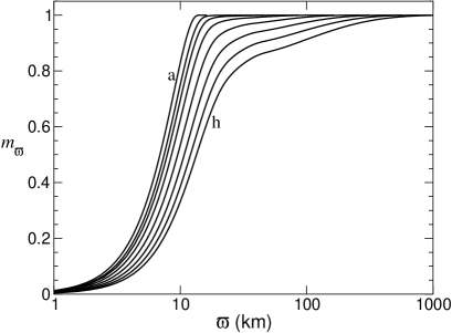
FIG. 5.: The cylindrical mass fraction $m_{\varpi}$ as a function of $\varpi$ for neutron star models in Fig. 4. The curves and their corresponding models are identified by the degree of central condensation: the higher the degree of central condensation, the lower the value of $\beta$.

FIG. 6.: The value of $\beta_{\varpi}$ as a function of $\varpi$ for the neutron star models in Fig. 4. The curves for models (a)-(g) terminate at the equatorial radii of the stars.

Figure 4 shows the rotational angular velocity $\Omega$ as a function of radius $\varpi$ for neutron star models corresponding to the collapse of sequence III white dwarfs. The cases for sequences I and II are similar. We see that stars with small $\beta$ show strong differential rotation. However, the rotation in the core region ($\varpi\stackrel{{\scriptstyle<}}{{{}_{\sim}}}20~{}\rm{km}$) becomes more and more rigidly rotating as $\beta$ increases. The most rapidly rotating case ($\beta=0.261$) has $\Omega\approx 4400~{}\rm{rad}~{}\rm{cm}^{-1}$ in the core. This corresponds to a rotation period of 1.4 ms, slightly less than the period of the fastest observed millisecond pulsar (1.56 ms). Further analysis reveals that the rotation curve in the envelope region roughly follows the Kepler law $\Omega\propto\varpi^{-3/2}$.

Figure 5 shows the cylindrical mass fraction $m_{\varpi}$ as a function of $\varpi$ for the same models as in Fig. 4. As expected, the degree of central concentration decreases with increasing $\beta$. However, more than 80% of the mass is still concentrated inside a radius $\varpi=30~{}\rm{km}$, even for the most rapidly rotating case. The collapsed object can be regarded as a rotating neutron star surrounded by an accretion torus.

Numerous numerical studies demonstrate that the quantity $\beta$ is an important parameter for the dynamical stability of a rotating star. It is then useful to define a function $\beta_{\varpi}$ as

$$\beta_{\varpi}=\frac{\int_{0}^{\varpi}d\varpi^{\prime}\,\varpi^{\prime}\int_{-\infty}^{\infty}dz^{\prime}\,[\varpi^{\prime}\Omega(\omega^{\prime})]^{2}\rho(\varpi^{\prime},z^{\prime})}{|\int_{0}^{\varpi}d\varpi^{\prime}\,\varpi^{\prime}\int_{-\infty}^{\infty}dz^{\prime}\,\rho(\varpi^{\prime},z^{\prime})\Phi(\varpi^{\prime},z^{\prime})|}\ ,$$ (8)

which is a measure of $\beta$ for the material inside a cylinder of radius $\varpi$ from the rotation axis. Figure 6 plots $\beta_{\varpi}$ as a function of $\varpi$ for the same neutron star models as in Fig. 4. We see that the curves level off when $\varpi\stackrel{{\scriptstyle>}}{{{}_{\sim}}}20-100~{}\rm{km}$ for all rapidly rotating models, suggesting that the material outside 100 km is probably unimportant for dynamical stability. It should also be noticed that the major contribution to $\beta$ is from the region $10~{}\rm{km}\stackrel{{\scriptstyle<}}{{{}_{\sim}}}\varpi\stackrel{{\scriptstyle<}}{{{}_{\sim}}}50~{}\rm{km}$. Hence we expect that the material in this region plays an important role on the dynamical stability of the star.

III Stability of the Collapsed Objects

In this Section, we study the dynamical stabilities of the neutron star models computed in Sec. II B using the technique of the linear stability analysis developed by Toman et al [29]. This technique is briefly reviewed in Sec. III A. We then report the stability results in Sec. III B.

A Linear stability analysis

The motion of fluid inside the star is described by the hydrodynamical equations:

$$\partial_{t}\rho+\nabla_{a}(\rho v^{a}) = 0\ ,$$ (9)

$$\partial_{t}v^{a}+v^{b}\nabla_{b}v^{a} = -\frac{\nabla^{a}P}{\rho}-\nabla^{a}\Phi\ ,$$ (10)

$$\nabla_{a}\nabla^{a}\Phi=4\pi G\rho\ ,$$ (11)

where the summation convention is assumed, and $\nabla_{a}$ denotes the covariant derivative compatible with three-dimensional flat-space metric. To study the stability, we perturb the density $\rho$ and velocity $v^{a}$ away from their equilibrium values by small quantities:

$$\rho(x^{b},t) = \rho_{0}(x^{b})+\delta\rho(x^{b},t)\ ,$$ (12)

$$v^{a}(x^{b},t) = \varpi\Omega(\varpi)e^{a}_{\hat{\varphi}}+\delta v^{a}(x^{b},t)\ ,$$ (13)

where $e^{a}_{\hat{\varphi}}$ is the unit vector along the azimuthal direction. The Lagrangian pressure perturbation $\Delta P$ is related to the Lagrangian density perturbation $\Delta\rho$ by

$$\Delta P=\gamma_{p}\frac{P}{\rho}\Delta\rho\ ,$$ (14)

where for simplicity, the subscript “0” is suppressed, and hereafter in this Section, $\rho$ and $P$ denote the equilibrium density and pressure respectively. The quantity

$$\gamma_{p}=\left(\frac{d\log P}{d\log\rho}\right)_{p}$$ (15)

is the adiabatic index for pulsation. The relation between the Eulerian perturbations $\delta P$ and $\delta\rho$ can be easily deduced from the transformation between the Lagrangian and Eulerian perturbations. The result is

$$\delta P=\gamma_{p}\frac{P}{\rho}\delta\rho+\left(\frac{\gamma_{p}}{\gamma_{\rm eq}}-1\right)\xi^{a}\nabla_{a}P\ ,$$ (16)

where

$$\gamma_{\rm eq}=\left(\frac{d\log P}{d\log\rho}\right)_{\rm eq}$$ (17)

is the adiabatic index computed from the equilibrium EOS. The Langrangian displacement $\xi^{a}$ satisfies the equation

$$\partial_{t}\xi^{a}+v^{b}\nabla_{b}\xi^{a}-\xi^{b}\nabla_{b}v^{a}=\delta v^{a}\ .$$ (18)

The Eulerian change of the gravitational potential $\delta\Phi$ satisfies the Poisson equation

$$\nabla_{a}\nabla^{a}\delta\Phi=4\pi G\delta\rho\ .$$ (19)

We find it useful to introduce a quantity $\delta h\equiv\delta P/\rho$, which is related to $\delta\rho$ by

$$\delta h=\gamma_{p}\frac{P}{\rho^{2}}\delta\rho+\left(\frac{\gamma_{p}}{\gamma_{\rm eq}}-1\right)\xi^{a}\nabla_{a}h\ .$$ (20)

In the region where $\gamma_{p}=\gamma_{\rm eq}$, $\delta h$ is the Eulerian change of the enthalpy.

If the system is unstable, the perturbed quantities will grow in time. Instead of solving the fully non-linear equations (9)–(11), however, Toman et al [29] develop a more efficient approach: expand Eqs. (9)–(11) to linear order of the perturbations and evolve the linearized equations.

Consider the angular Fourier decomposition of any perturbed quantity $\delta q$:

$$\delta q(x^{b},t)=\sum_{m=-\infty}^{\infty}\delta\tilde{q}_{m}(\varpi,z,t)e^{im\varphi}\ .$$ (21)

It can be easily proved that each $m$-mode decouples in the linearized hydrodynamical equations because of the axisymmetry of the equilibrium configuration. In addition, the fact that the equilibrium configuration is symmetric under reflection about the equatorial plane ($z\rightarrow-z$) implies the modes with even and odd parity under the transformation $z\rightarrow-z$ also decouple. Hence each $m$-mode with a definite parity can be evolved separately and the 3+1 simulation is reduced to a 2+1 simulation, which saves a lot of computation time. Hereafter, all perturbed quantities will be assumed to have angular dependence $e^{im\varphi}$.

In Ref. [29], Toman et al choose to evolve the variables $\delta\rho$ and $\delta v^{a}$. However, we find it more convenient and numerically stable in our case to evolve the variables $\delta h$ and $\delta p^{a}=\rho\delta v^{a}$. The reason being that the simulations are performed on a discrete grid, and it is preferable to use variables that change smoothly to ensure accuracy. However, the background density $\rho$ decreases abruptly outside the core region, and the perturbation $\delta\rho$ is expected to behave similarly. On the other hand, $h$, and presumably $\delta h$, change much more smoothly even near the boundary of the star. In the case where $\gamma_{p}\neq\gamma_{\rm eq}$, we also need to evolve the scalar function $\eta=\xi^{b}\nabla_{b}h$. In terms of the new variables, the linearized equations become

$$\partial_{t}\delta h = -im\Omega\delta h-\gamma_{p}\frac{P}{\rho^{2}}\nabla_{a}\delta p^{a}$$ (23)

$$+\left(\frac{\gamma_{p}}{\gamma_{\rm eq}}-1\right)\frac{\delta p^{a}}{\rho}\nabla_{a}h\ ,$$

$$\partial_{t}\delta p^{a} = -\delta p^{b}\nabla_{b}v^{a}-v^{b}\nabla_{b}\delta p^{a}-\rho\nabla^{a}\delta h-\rho\nabla^{a}\delta\Phi$$ (25)

$$-\left(\frac{\gamma_{p}}{\gamma_{\rm eq}}-1\right)\frac{\rho^{2}}{\gamma_{p}P}(\delta h+\eta)\nabla^{a}h\ ,$$

$$\partial_{t}\eta = -im\Omega\eta+\frac{\delta p^{a}}{\rho}\nabla_{a}h\ ,$$ (26)

$$\nabla_{a}\nabla^{a}\delta\Phi = \frac{4\pi G\rho^{2}}{\gamma_{p}P}\left[\delta h-\left(\frac{\gamma_{p}}{\gamma_{\rm eq}}-1\right)\eta\right]\ .$$ (27)

It follows from Eqs. (23)–(27) that if $(\delta h,\delta p^{a})$ is a solution for an $m$-mode, the complex conjugate $(\delta h^{*},{\delta p^{a}}^{*})$ is a solution for the -$m$-mode. We can then define the physical “enthalpy” perturbation $\delta\tilde{h}=\delta h+\delta h^{*}$, and similarly for the physical density $\delta\tilde{\rho}$ and velocity $\delta\tilde{v}^{a}$ perturbations of an $m$-mode.

We use a uniform cylindrical grid to perform the simulations. We have checked that the code is able to reproduce the results in Ref. [29]. However, unlike the case in Ref. [29], the collapsed objects studied here have a large envelope extending beyond 1000 km when the stars under consideration are rapidly rotating. This numerical difficulty can be circumvented by a suitable truncation scheme.

As pointed out in Sec. II B, we expect the outer envelope will not influence the dynamical stability in any significant way. Hence it is necessary to evolve the perturbations only in the dynamically interesting region. This is done by introducing a radius $R_{m}$ and a minimum density $\rho_{\rm{min}}\equiv\rho(R_{m},0)$. The perturbations are set to zero wherever the equilibrium density $\rho(\varpi,z)<\rho_{\rm{min}}$. If $R_{m}$ is sufficiently large, increasing its value will not change the evolution result. We find that a value of $R_{m}\approx 200~{}\rm{km}$ is needed to ensure that the results converge, and we use a cylindrical grid with $400\times 400$ grid points to achieve a resolution of 0.5 km.

In general, the two adiabatic indices $\gamma_{p}$ and $\gamma_{\rm{eq}}$ are not equal. They coincide only if the pulsation timescale is much longer than all the reaction timescales for the different species of particles in the fluid to achieve equilibrium. This is the case for densities below neutron drip ($\rho\stackrel{{\scriptstyle<}}{{{}_{\sim}}}4\times 10^{11}~{}\rm{g}~{}\rm{cm}^{-3}$) and above about $10^{13}~{}\rm{g}~{}\rm{cm}^{-3}$. However, in the density range $4\times 10^{11}~{}\rm{g}~{}\rm{cm}^{-3}\stackrel{{\scriptstyle<}}{{{}_{\sim}}}\rho\stackrel{{\scriptstyle<}}{{{}_{\sim}}}10^{13}~{}\rm{g}~{}\rm{cm}^{-3}$, the matter is a mixture of electrons, neutrons and nuclei in equilibrium. Some of the reactions required to achieve equilibrium involve weak interactions, which have timescales much longer than the pulsation timescale. Hence equilibrium is not achieved during pulsation, and $\gamma_{p}\neq\gamma_{\rm{eq}}$ in that density range [30, 31]. Most people studying neutron star pulsations neglect the difference of $\gamma_{p}$ and $\gamma_{\rm{eq}}$ and use $\gamma_{\rm{eq}}$ in their calculations. It has been demonstrated (see e.g. [33]) that this treatment has no significant effect on the final result, because the matter in that density range occupies only a tiny fraction of neutron star. However, it may have an important effect on the stability of the new-born neutron stars studied here. The reason is that the dynamically important region, as pointed out in Sec. II B, is $10~{}\rm{km}\stackrel{{\scriptstyle<}}{{{}_{\sim}}}\varpi\stackrel{{\scriptstyle<}}{{{}_{\sim}}}50~{}\rm{km}$. This region contains a significant amount of matter in that density range (see Fig. 3). Our numerical simulations indicate that this is indeed the case. The critical value $\beta_{d}$ for the dynamical instability drops from about 0.25 to 0.23 if $\gamma_{\rm{eq}}$ is used for the adiabatic index of pulsation.

FIG. 7.: The values of $\gamma_{\rm eq}$ (solid line) and $\gamma_{p}$ (dashed line) as a function of $\log_{10}\rho$. The two curves coincide when $\rho<\rho_{d}$ and $\rho>\rho_{e}$.

The appropriate $\gamma_{p}$ remains roughly constant from the density of neutron drip $\rho_{d}=4\times 10^{11}~{}\rm{g}~{}\rm{cm}^{-3}$ to the density above which $\gamma_{\rm{eq}}=\gamma_{p}$ around $\rho_{e}=10^{13}~{}\rm{g}~{}\rm{cm}^{-3}$ [30, 31]. To provide a reasonable value of $\gamma_{p}$ which mimics the curve in Refs. [30, 31] and which is compatible with the EOS used here, we take $\gamma_{p}$ in the density range $\rho_{d}<\rho<\rho_{e}$ to be (also see Fig. 7)

$$\gamma_{p}(\rho)=\gamma_{\rm{eq}}(\rho_{d})+\left[\gamma_{\rm{eq}}(\rho_{e})-\gamma_{\rm{eq}}(\rho_{d})\right]\frac{\log^{2}(\rho/\rho_{d})}{\log^{2}(\rho_{e}/\rho_{d})}\ .$$ (28)

Under some circumstances it is possible to have a region of the star where the mode is stationary in the fluid’s co-rotating frame. In this case, we should use $\gamma_{\rm{eq}}$ for the adiabatic index of pulsation in the region where $|\omega^{\prime}|=|\omega+m\Omega|\ll 2\pi/t_{r}$. Here $\omega$ is the angular frequency of an $m$-mode that has dependence $\exp[i(\omega t+m\varphi)]$ in the inertial frame; $\omega^{\prime}=\omega+m\Omega$ is the angular frequency of the mode in the fluid’s co-rotating frame; and $t_{r}\approx 1~{}\rm{s}$ is the timescale for different species of particles to achieve $\beta$-equilibrium in the density range $\rho_{d}<\rho<\rho_{e}$. It turns out (see the next subsection) that rapidly rotating neutron stars have an unstable bar mode ($m=2$) with $\omega\approx-3000~{}\rm{rad}~{}\rm{s}^{-1}$. There is indeed a radius at which $\omega^{\prime}=0$. This radius is at $\varpi=\varpi_{c}\approx 40~{}\rm{km}$ for stars with $\beta>0.23$. The density on the equator of the stars is $\rho\approx 10^{12}~{}\rm{g}~{}\rm{cm}^{-3}$, well within the questionable density range. However, the width of this “co-rotating region” which satisfies $|\omega^{\prime}|<2\pi/t_{r}$ is

$\displaystyle\Delta\varpi=\frac{2\pi/t_{r}}{\left|\partial_{\varpi}\Omega(\varpi_{c})\right|}\approx 0.1~{}\rm{km}\ .$

The material in the region contains only $10^{-4}$ of total mass and angular momentum of the star. Hence this thin co-rotating layer is not expected to have a significant influence on the overall stability of the stars.

B Results

We perform a number of simulations on neutron star models computed by the method described in Sec. II B. The simulations are terminated either when an instability is fully developed or when the simulation time reaches 60 ms, corresponding to 40 rotation periods of the material at the center of the star. We regard a star as dynamically unstable if the density perturbation shows an evidence of exponential growth and increases its amplitude by at least a factor of fifteen by the end of the simulation. In our simulations, no instability is observed for neutron star models in sequences I and II. A bar-mode ($m=2$) instability develops for sequence III models when the star’s $\beta$ is greater than a critical value $\beta_{d}\approx 0.25$. The unstable mode has even parity under reflection about the equatorial plane. This $\beta_{d}$ is slightly less than the critical value 0.27 for the Maclaurin spheroids. It should be pointed out that all the stars in sequences I and II have $\beta$’s smaller than this $\beta_{d}$. Hence we believe that they are stable simply because their $\beta$’s are not high enough.

Some other simulations [9, 13] show that in the cases where $\beta_{d}<0.27$, the instability is dominated by the $m=1$ mode for stars with $\beta$ close to $\beta_{d}$. However, we do not observe any sign of an unstable $m=1$ mode in our case. We also performed simulations using $\gamma_{\rm eq}$ (the solid curve in Fig. 7) as the adiabatic index for pulsation instead of $\gamma_{p}$ (the dashed curve in Fig. 7). We find that $\beta_{d}$ drops to about 0.23, showing that matter in the density region $\rho_{d}<\rho<\rho_{e}$ plays an important role on the instability.

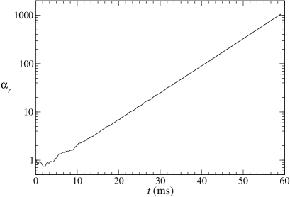
FIG. 8.: The relative amplitude $\alpha_{r}$ as a function of time. The equilibrium star has $\beta=0.261$, the most rapidly rotating model.

To visualize the instability, we define an amplitude

$$\alpha=\left(\frac{\int|\delta\rho|^{2}\,d^{3}x}{\int\rho^{2}\,d^{3}x}\right)^{1/2}$$ (29)

for the density perturbation. Since we evolve the perturbations using linearized equations, it is more convenient to work with the relative amplitude $\alpha_{r}$:

$$\alpha_{r}(t)=\alpha(t)/\alpha(0)\ .$$ (30)

This relative amplitude is defined so that it is equal to one at $t=0$. Figure 8 shows the time evolution of $\alpha_{r}$ for the most rapidly rotating star ($\beta=0.261$). We see that after about 10 ms, an instability develops and $\alpha_{r}$ grows exponentially. The e-folding time of the growth $\tau$ is found, by least square fit, to be 7.8 ms.

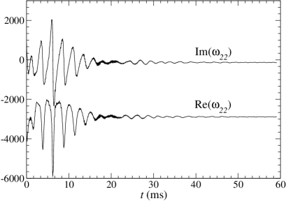
FIG. 9.: The time evolution of the angular frequency $\omega_{22}$ for the most rapidly rotating star ($\beta=0.261$).

The unstable mode can also be characterized by a complex angular frequency defined as

$$\omega_{22}=\frac{\dot{D}_{22}}{iD_{22}}\ ,$$ (31)

where

$$D_{22}=\int r^{2}\delta\rho Y^{*}_{22}\,d^{3}x$$ (32)

is the mass quadrupole moment, and the spherical harmonic function

$\displaystyle Y_{22}=\frac{1}{4}\sqrt{\frac{15}{2\pi}}\,\sin^{2}\theta\,e^{2i\varphi}\ .$

The time derivative of $D_{22}$ is evaluated by the formula [32]

$$\dot{D}_{22}=\int\delta p^{a}\nabla_{a}(r^{2}Y^{*}_{22})\,d^{3}x-2i\int\Omega r^{2}\delta\rho Y^{*}_{22}\,d^{3}x\ ,$$ (33)

where we have used the continuity equation (9) and integrated by parts.

Let $\omega$ be the complex frequency of the most unstable mode. The e-folding time is related to the imaginary part of $\omega$ by $\rm{Im}(\omega)=-1/\tau$. At late time, the density perturbation is dominated by the most unstable mode, which means that both $\delta\rho$ and $D_{22}$ go approximately as $\exp(i\omega t)$. Hence $\omega_{22}\approx\omega$. Fig. 9 plots $\omega_{22}$ as a function of time for the evolution of the most rapidly rotating star. We see that at late time, $\omega_{22}$ is approximately a constant, indicating that the perturbation is indeed dominated by the most unstable mode. The frequency of the unstable mode is then determined to be $\omega\approx(-2890-130i)~{}\rm{rad}~{}\rm{s}^{-1}$. Note that the imaginary part agrees with the e-folding time determined above.

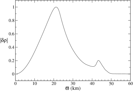
FIG. 10.: The magnitude of the density perturbation $|\delta\rho|$ of the unstable bar mode of the most rapidly rotating star ($\beta=0.261$) on the equatorial plane. The magnitude is normalized so that the maximum value is one.

Figure 10 shows the magnitude of the density perturbation $|\delta\rho|$ of the unstable bar mode of the most rapidly rotating star ($\beta=0.261$) on the equatorial plane. We see that $|\delta\rho|$ has a peak at $\varpi\approx 20~{}{\rm km}$, which is in the transition region between the neutron star core and the tenuous outer layers (see Fig. 3). There is a small, secondary peak at $\varpi=44~{}{\rm km}$, which is the corotation radius at which $\mbox{Re}(\omega)+2\Omega=0$ for this neutron star. This secondary peak is caused by the resonant response of the fluid being driven by the mode corotating with it (see Appendix A).

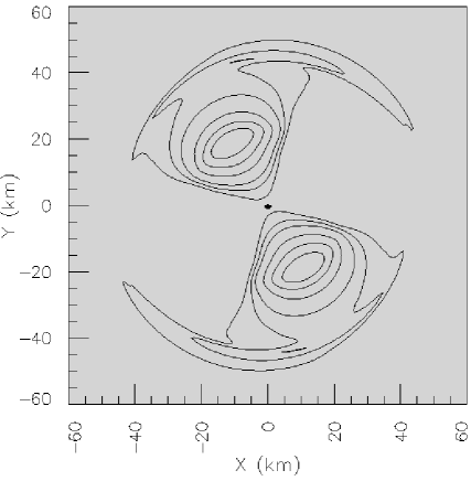
FIG. 11.: The eigenfunction of the physical density perturbation $\delta\tilde{\rho}$ on the equatorial plane for the bar mode of the most rapidly rotating star ($\beta=0.261$). The density perturbations are normalized so that the maximum value is one. Only positive density regions of the eigenfunction are shown. The negative structure of the eigenfunction can be inferred from the sinusoidal structure of the eigenfunction. The contour levels are, from inward to outward, 0.8, 0.6, 0.4, 0.2, 0.1 and 0.01. The small arcs inside the 0.1 contours are additional contours of 0.2, corresponding to the secondary peak in Fig. 10.

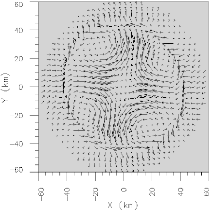
FIG. 12.: The eigenfunction of the physical velocity perturbation $\delta\tilde{v}^{a}$ on the equatorial plane for the bar mode of the most rapidly rotating star ($\beta=0.261$).

Figures 11 and 12 show the eigenfunctions of the physical perturbations $\delta\tilde{\rho}$ and $\delta\tilde{v}^{a}$ on the equatorial plane. Note that our grid extends out to 200 km from the center, but the dynamically interesting region is concentrated within 60 km from the center. Since the time dependence of the perturbations go as $\exp[i(\omega t+m\varphi)]$, $\rm{Re}(\omega)<0$ means the pattern rotates in prograde (counter-clockwise) direction. The density perturbation is bar-like in the inner region and becomes trailing spirals in the outer region. Similar structure is also observed in other numerical simulations on the bar-mode instability [9, 29, 8, 10, 11, 7, 34]. The secondary peak of $\delta\rho$ appears as two small arcs in Fig. 11 just inside the 0.1 contours. Figure 12 shows that $\delta\tilde{v}^{a}$ is almost parallel to the $\varphi$ direction at the corotation radius, which is also a result of resonance (see Appendix A). Since $\delta\tilde{v}^{a}$ changes abruptly near the corotation radius, it is very possible that shocks will develop there when the perturbations become large. This might have significant influence on the non-linear evolution of the bar mode.

TABLE II.: The oscillation frequency $f$ and e-folding time $\tau$ of the most unstable bar mode for several unstable neutron stars. Here $\Omega$ is the rotational frequency of the pre-collapse white dwarf, and $\Omega_{m}$ is the maximum frequency of the white dwarf in Sequence III.

$(\Omega/\Omega_{m})_{WD}$	$\beta$	Re($-\omega$)	$f$	$\tau$
		$\rm{rad}~{}\rm{s}^{-1}$	Hz	ms
0.934	0.251	2800	445	20
0.964	0.255	2850	450	12
0.989	0.258	2850	450	8.9
1.000	0.261	2890	460	7.8

The eigenfunctions of the most unstable bar mode for the other unstable equilibrium neutron stars are similar to those displayed above. Table II summarizes the oscillation frequencies [$f=|\rm{Re}(\omega)|/(2\pi)$] and e-folding time $\tau$ of the unstable models we have studied. The table also shows the ratio of the rotational frequency of the pre-collapse white dwarfs to the maximum frequency $\Omega_{m}$ of the white dwarf in the sequence. We find that the oscillation frequencies are almost the same ($\approx 450~{}\rm{Hz}$) for all the cases. We do not observe any instability in our simulations for stars with $\beta\leq 0.241$. Hence we conclude that $\beta_{d}$ is somewhere between 0.241 and 0.251, and the pre-collapse white dwarf has to have $\Omega\stackrel{{\scriptstyle>}}{{{}_{\sim}}}0.93\Omega_{m}$ in order for the collapsed star to develop a dynamical instability.

IV Gravitational Radiation

In this section, we estimate the strength of the gravitational radiation emitted by neutron stars undergoing a dynamical instability. We also estimate the signal to noise ratio and discuss the detectability of these sources.

The rms amplitude of a gravitational wave strain, $h(t)$, depends on the orientation of the source and its location on the detector’s sky. When averaged over these angles, its value is given by [36]

$$h^{2}(t)=\frac{1}{5}\langle h^{2}_{+}(t)+h^{2}_{\times}(t)\rangle\ ,$$ (34)

where $h_{+}(t)$ and $h_{\times}(t)$ are the rms amplitudes of the plus and cross polarizations of the wave respectively, and $\langle...\rangle$ denotes an average over the orientation of the source and its location on the detector’s sky.

In the presence of perturbations, the density and velocity of fluid inside the star become

$$\rho(\mbox{\boldmath$x$},t) = \rho_{0}(\varpi,z)+\sum_{m=-\infty}^{\infty}\delta\rho_{m}(\mbox{\boldmath$x$},t)$$ (35)

$$\mbox{\boldmath$v$}(\mbox{\boldmath$x$},t) = \varpi\Omega(\varpi)\mbox{\boldmath$e_{\hat{\varphi}}$}+\sum_{m=-\infty}^{\infty}\delta\mbox{\boldmath$v$}_{m}(\mbox{\boldmath$x$},t)\ ,$$ (36)

where the perturbation functions $\delta\rho_{m}$ and $\delta\mbox{\boldmath$v$}_{m}$ have angular dependence $e^{im\varphi}$. The amplitude of the gravitational waves produced by time varying mass and current multipole moments can be derived from Ref. [37]. The result is

$$h^{2}=\frac{1}{D^{2}}\sum_{l=2}^{\infty}\sum_{m=-l}^{l}\frac{4G^{2}}{5c^{2l+4}}N_{l}\left[|D^{(l)}_{lm}|^{2}+|S_{lm}^{(l)}|^{2}\right]$$ (37)

where $D$ is the distance between the source and detector; $c$ is the speed of light, and

$$N_{l} = \frac{4\pi(l+1)(l+2)}{l(l-1)[(2l+1)!!]^{2}}\ ;$$ (38)

$$D_{lm}^{(l)} = \frac{d^{l}}{dt^{l}}D_{lm}\ ;$$ (39)

$$S_{lm}^{(l)} = \frac{d^{l}}{dt^{l}}S_{lm}\ .$$ (40)

For a Newtonian source, the mass moments $D_{lm}$ and current moments $S_{lm}$ are given by

$$D_{lm} = \int\rho r^{l}Y_{lm}^{*}\,d^{3}x$$ (41)

$$S_{lm} = \frac{2}{c}\sqrt{\frac{l}{l+1}}\int r^{l}\rho\mbox{\boldmath$v$}\cdot\mbox{\boldmath$Y^{B}_{lm}$}^{*}\,d^{3}x\ ,$$ (42)

where $\mbox{\boldmath$Y^{B}_{lm}$}=\mbox{\boldmath$x$}\times\mbox{\boldmath$\nabla$}Y_{lm}/\sqrt{l(l+1)}$ are the magnetic type vector spherical harmonics. The functions $D_{lm}$ and $S_{lm}$ have the property that $D_{lm}^{*}=(-1)^{m}D_{l\,-m}$ and $S_{lm}^{*}=(-1)^{m}S_{l\,-m}$. Hence it is sufficient to consider only positive values of $m$ and Eq. (37) becomes

$$h^{2}=\frac{1}{D^{2}}\sum_{l=2}^{\infty}\sum_{m=0}^{l}\frac{8G^{2}}{5c^{2l+4}}N_{l}\left[|D^{(l)}_{lm}|^{2}+|S_{lm}^{(l)}|^{2}\right]\ .$$ (43)

The energy and angular momentum carried by the gravitational waves can also be derived from [37]. The result is

$$\dot{E} = \sum_{l=2}^{\infty}\sum_{m=0}^{l}\frac{G}{c^{2l+1}}\,2N_{l}\overline{\left[|D_{lm}^{(l+1)}|^{2}+|S_{lm}^{(l+1)}|^{2}\right]}\ ;$$ (44)

$$\dot{J} = \sum_{l=2}^{\infty}\sum_{m=0}^{l}\frac{G}{c^{2l+1}}\,2imN_{l}\overline{\left[D_{lm}^{(l)*}D_{lm}^{(l+1)}+S_{lm}^{(l)*}S_{lm}^{(l+1)}\right]}\ ,$$ (45)

where the overline denotes time average over several periods.

When a neutron star develops a dynamical instability and the bar mode ($m=2$) is the only unstable mode, the values of $h$, $\dot{E}$ and $\dot{J}$ will be dominated by the term involving $D_{22}$. Since the unstable bar mode has even parity under reflection about the equatorial plane, $D_{32}=S_{22}=0$ and the next leading term will involve $S_{32}$ and $D_{42}$. These terms are expected to be smaller than the $D_{22}$ term by a factor of $(v/c)^{4}$ for $\dot{E}$ and $\dot{J}$, and a factor of $(v/c)^{2}$ for $h$. In our models, $v/c<0.28$, so the contribution of higher order mass and current multipole moments are small and will be neglected.

Strictly speaking, the above analysis only applies when the amplitudes of the perturbations are small. When the amplitudes are large, however, the fluid motion does not separate neatly into decoupled Fourier components, so all $D_{lm}$ and $S_{lm}$ will contribute. However, it is expected that the $D_{22}$ term will still be the most important term. Since the detailed non-linear evolution of the dynamical instability is not known, the aim of this section is to provide an order of magnitude estimate of the gravitational radiation from these sources. Hence we shall only consider the effect of the mass quadrupole moment and assume $D_{22}$ can be approximated by the bar-mode eigenfunctions computed in Sec. III B. In this approximation, Eqs. (43)–(45) become

$$h = \frac{32\pi^{2}G}{5c^{4}D}f^{2}|D_{22}|\sqrt{\frac{\pi}{15}}\ ;$$ (46)

$$\dot{E} = \frac{1024\pi^{7}G}{75c^{5}}f^{6}|D_{22}|^{2}\ ;$$ (47)

$$\dot{J} = \frac{1024\pi^{6}G}{75c^{5}}f^{5}|D_{22}|^{2}\ ,$$ (48)

where $f=|\mbox{Re}(\omega)|/(2\pi)$ is the oscillation frequency of the bar mode.

Substituting the bar-mode eigenfunctions (from Sec. III B) into Eq. (41), we find that

$$|D_{22}|\approx\alpha\,8\times 10^{45}~{}\rm{g}~{}\rm{cm}^{2}$$ (49)

for all the unstable models we have studied. Here $\alpha$ is the amplitude of the bar mode defined in Eq. (29). The mass quadrupole moment $D_{22}$ has a time dependence $\exp(i\omega t)$, where $\omega$ is the angular frequency of the mode. Hence the time derivative $D_{22}^{(l)}=(i\omega)^{l}D_{22}$ and we obtain

$$h \approx \alpha\,7\times 10^{-23}\left(\frac{20~{}\rm{Mpc}}{D}\right)\ ;$$ (50)

$$\dot{E} \approx \alpha^{2}\,9\times 10^{52}~{}\rm{erg}~{}\rm{s}^{-1}\ ;$$ (51)

$$\dot{J} \approx \alpha^{2}\,6\times 10^{49}~{}\rm{g}~{}\rm{cm}^{2}~{}\rm{s}^{-2}\ .$$ (52)

The signal to noise ratio of these sources depends on the detailed evolution of the bar mode when the density perturbation reaches a large amplitude and non-linear effects take over. Recently, New, Centrella and Tohline [11] and Brown [35] perform long-duration simulations of the bar-mode instability. They find that the mode saturates when the density perturbation is comparable to the equilibrium density, and the mode pattern persists, giving a long-lived gravitational wave signal. Here we assume that this is the case, and that the mode dies out only after a substantial amount of angular momentum is removed from the system by gravitational radiation. We then follow the method described in Refs. [38, 39] to estimate the signal to noise ratio.

In the stationary phrase approximation, the gravitational wave in the frequency domain $\tilde{h}(f)$ is related to $h(t)$ by

$$h^{2}(t)=|\tilde{h}(f)|^{2}\left|\frac{df}{dt}\right|\ .$$ (53)

Combining Eqs. (46), (48) and (53), we obtain

$$|\tilde{h}(f)|^{2}=\frac{G}{c^{3}}\frac{\dot{J}}{5\pi f|\dot{f}|D^{2}}\ .$$ (54)

The signal to noise ratio is given by

$$\left(\frac{S}{N}\right)^{2}=2\int_{0}^{\infty}\frac{|\tilde{h}(f)|^{2}}{S_{h}(f)}\,df\ ,$$ (55)

where $S_{h}(f)$ is the spectral density of the detector’s noise. If we assume that the oscillation frequency remains constant in the entire evolution, we obtain [40]

$$\frac{S}{N}=\frac{1}{D}\sqrt{\frac{2G}{5\pi c^{3}}\frac{\Delta J}{fS_{h}(f)}}\ ,$$ (56)

where $\Delta J$ is the total amount of angular momentum emitted by gravitational waves. To estimate $\Delta J$, we assume that the mode dies out when the angular momentum of the star decreases to $J_{d}\approx 3.3\times 10^{49}~{}\rm{g}~{}\rm{cm}^{2}~{}\rm{s}^{-1}$, which is the angular momentum of the marginally bar-unstable star. Then we have $\Delta J\stackrel{{\scriptstyle<}}{{{}_{\sim}}}5\times 10^{48}~{}\rm{g}~{}\rm{cm}^{2}~{}\rm{s}^{-1}$ for all the unstable stars, and the signal to noise ratio for LIGO-II broad-band interferometers [41] is

$$\frac{S}{N} = 15\left(\frac{20~{}\rm{Mpc}}{D}\right)\left(\frac{\Delta J}{5\times 10^{48}~{}\rm{cgs}}\right)^{1/2}\times$$ (58)

$$\left(\frac{f}{450~{}\rm{Hz}}\right)^{-1/2}\left(\frac{\sqrt{S_{h}(f)}}{2\times 10^{-24}~{}\rm{Hz}^{-1/2}}\right)^{-1}\ .$$

The timescale of the gravitational wave emission can be estimated by the equation

$$\tau_{GW} \sim \frac{\Delta J}{\dot{J}}$$ (59)

$$\sim 7~{}\rm{s}\,\left(\frac{\alpha_{s}}{0.1}\right)^{-2}\left(\frac{\Delta J}{5\times 10^{48}~{}\rm{cgs}}\right)\ ,$$ (60)

where $\alpha_{s}$ is the amplitude $\alpha$ of the density perturbation at which the mode saturates. We have used Eqs. (48) and (49) to calculate the numerical value in the last equation.

The detectability of this type of sources also depends on the event rate. The event rate for the AIC in a galaxy is estimated to be between $10^{-5}$ and $10^{-8}$ per year [42, 43]. Of all the AIC events, only those corresponding to the collapse of rapidly rotating O-Ne-Mg white dwarfs can end up in the bar-mode instability, and the fraction of which is unknown. If a signal to noise ratio of 5 is required to detect the source, an event rate of at least $10^{-6}$/galaxy/year is required for such a source to occur at a detectable distance per year. Hence these sources will not be promising for LIGO II if the event rate is much less than $10^{-6}$ per year per galaxy.

The event rate of the core collapse of massive stars is much higher than that of the AIC. The structure of a pre-supernova core is very similar to that of a pre-collapse white dwarf, so our results might be applicable to the neutron stars produced by the core collapse. If the core is rapidly rotating, the resulting neutron star might be able to develop a bar-mode instability. If a significant fraction of the pre-supernova cores are rapidly rotating, the chance of detecting the gravitational radiation from the bar-mode instability might be much higher than expected.

V Magnetic Field Effects

As mentioned in Sec. II B, a new-born hot proto-neutron star is dynamically stable because its $\beta$ is too small. It takes about 20 s for the proto-neutron star to cool down and evolve into a cold neutron star, which may have high enough $\beta$ to trigger a dynamical instability. The proto-neutron stars, as well as the cold neutron stars computed in Sec. II B, show strong differential rotation (Paper I). This differential rotation will cause a frozen-in magnetic field to wind up, creating strong toroidal fields. This process will result in a re-distribution of angular momentum and destroy the differential rotation. If the timescale of this magnetic braking is shorter than the cooling timescale, the star may not be able to develop the dynamical instability discussed in Secs. III and IV. In this Section, we estimate the timescale of this magnetic braking.

In the ideal magnetohydrodynamics limit, the magnetic field lines are frozen into the moving fluid. The evolution of magnetic field $B$ is governed by the induction equation

$$\frac{\partial B^{a}}{\partial t}+v^{b}\nabla_{b}B^{a}-B^{b}\nabla_{b}v^{a}=-B^{a}\nabla_{b}v^{b}\ .$$ (61)

In our equilibrium models, $v^{b}=\varpi\Omega(\varpi)e^{b}_{\hat{\varphi}}$. Hence $\nabla_{b}v^{b}=0$ and Eq. (61) becomes

$$\frac{dB^{a}}{dt}=B^{b}\nabla_{b}v^{a}\ ,$$ (62)

where $d/dt=\partial/\partial t+v^{b}\nabla_{b}$ is the time derivative in the fluid’s co-moving frame. Eq. (62) can be integrated analytically (see e.g. Appendix B of [44]). The magnetic field $B^{j}(\mbox{\boldmath$x$},t)$ at the position $x$ of a fluid element at time $t$ is related to the magnetic field $B^{k}(\mbox{\boldmath$x_{0}$},t_{0})$ at the position $x_{0}$ of the same fluid at time $t_{0}$ by

$$B^{j}(\mbox{\boldmath$x$},t)=B^{k}(\mbox{\boldmath$x_{0}$},t_{0})\frac{\partial x^{j}}{\partial x_{0}^{k}}\ ,$$ (63)

where $\partial x^{j}/\partial x_{0}^{k}$ is the coordinate strain between $t_{0}$ and $t$. With $v^{a}=\varpi\Omega(\varpi)e^{a}_{\hat{\varphi}}$, it is easy to show that the induced magnetic field has components only in the $e^{a}_{\hat{\varphi}}$ direction. Its magnitude $B_{i}$, after a time $t$, is easy to compute from Eq. (63). The result is

$$B_{i}(t)=B_{0}t\varpi|\partial_{\varpi}\Omega|\ ,$$ (64)

where $B_{0}$ is the component of magnetic field in the $\mbox{\boldmath$e$}_{\varpi}$ direction. The induced magnetic field will significantly change the equilibrium velocity field when the energy density of magnetic field $\epsilon_{B}=B_{i}^{2}/(8\pi)$ is comparable to the rotational kinetic energy density $\epsilon_{R}=\rho\varpi^{2}\Omega^{2}/2$. This will occur in a timescale $\tau_{B}$ set by $\epsilon_{B}=\epsilon_{R}$. Using Eq. (64), we obtain

$$\tau_{B}=\frac{\Omega}{|\partial_{\varpi}\Omega|}\,\frac{\sqrt{4\pi\rho}}{B_{0}}=\frac{L}{v_{A}}\ ,$$ (65)

where $L=\Omega/|\partial_{\varpi}\Omega|$ is the length scale of differential rotation, and $v_{A}=B_{0}/\sqrt{4\pi\rho}$ is the speed of Alfvèn waves.

Observational data suggest that the magnetic fields of most white dwarfs are smaller than $10^{5}~{}\rm{G}$, although a small fraction of “magnetic white dwarfs” can have fields in the range $10^{6}-10^{9}~{}\rm{G}$. Assuming flux conservation, the magnetic fields of the hot proto-neutron stars just after collapse would be $B_{0}\sim 10^{9}~{}\rm{G}$ for those $10^{5}~{}\rm{G}$ white dwarfs. Using the angular velocity distribution in Paper I for the hot proto-neutron star, we find that the magnetic timescale in the dynamically important region ($\varpi\stackrel{{\scriptstyle<}}{{{}_{\sim}}}100~{}\rm{km}$) is

$$\tau_{B}\approx 10^{4}~{}\mbox{s}\,\left(\frac{10^{9}~{}\mbox{G}}{B_{0}}\right)\ ,$$ (66)

which is much longer than the neutrino cooling timescale ($\sim 20~{}\rm{s}$). Hence the angular momentum transport caused by the magnetic field is negligible during the cooling period. The magnetic timescale for the cold neutron stars can be calculated from the angular frequency distribution computed in Sec. II B. We find that $\tau_{B}$ for the cold models is about half of that given by Eq. (66), which is still much longer than the timescale of gravitational waves $\tau_{GW}$ calculated in the previous Section. The instability results presented in the previous two Sections remain unchanged unless the neutron star’s initial magnetic field $B_{0}$ is greater than $10^{12}~{}\rm{G}$. In that case, a detailed magnetohydrodynamical simulation has to be carried out to compute the angular momentum transport.

The magnetic timescale for these nascent neutron stars is significantly different from that estimated by Baumgarte, Shapiro and Shibata [45] and Shapiro [46]. They consider differentially rotating “hypermassive” neutron stars, which could be the remnants of the coalescence of binary neutron stars. Those neutron stars are very massive ($M\sim 3M_{\odot}$) and have much higher densities than the new-born neutron stars studied in this paper. They also use a seed magnetic field of strength $B_{0}\sim 10^{12}~{}\rm{G}$, which is much larger than our estimate. These two differences combined make our magnetic braking timescale two orders of magnitude larger than theirs. It should be noted that it is the magnetic field just after the collapse that is relevant to our analysis here. The strong differential rotation of the neutron star will eventually generate a very strong toroidal field ($B_{i}\sim 10^{16}~{}\rm{G}$) and destroy the differential rotation. The final state of the neutron star will be in rigid rotation, and its magnetic field will be completely different from the initial field. For this reason, the field strength $B\sim 10^{12}~{}\rm{G}$ observed in a typical pulsar is probably not relevant here.

VI Summary and Discussion

We have applied linear stability analysis to study the dynamical stability of new-born neutron stars formed by AIC. We find that a neutron star has a dynamically unstable bar mode if its $\beta$ is greater than the critical value $\beta_{d}\approx 0.25$. In order for the neutron star to have $\beta>\beta_{d}$, the pre-collapse white dwarf must be composed of oxygen, neon, magnesium and have a rotational angular frequency $\Omega\stackrel{{\scriptstyle>}}{{{}_{\sim}}}3.4~{}\rm{rad}~{}\rm{s}^{-1}$, corresponding to 93% of the maximum rotational frequency the white dwarf can have without mass shedding.

The eigenfunction of the most unstable bar mode is concentrated within a radius $\varpi\stackrel{{\scriptstyle<}}{{{}_{\sim}}}60~{}\rm{km}$. The oscillation frequency of the mode is $f\approx 450~{}\rm{Hz}$. When the amplitude of the mode is small, it grows exponentially with an e-folding time $\tau\approx 8~{}\rm{ms}$ for the most rapidly rotating star ($\beta=0.261$), which is about 5.5 rotation periods at the center of the star.

The signal to noise ratio of the gravitational waves emitted by this instability is estimated to be 15 for LIGO-II broad-band interferometers if the source is located in the Virgo cluster of galaxies ($D=20~{}\rm{Mpc}$). The detectability of these sources also depends on the event rate. The event rate of AIC is between $10^{-5}$ and $10^{-8}/\rm{galaxy}/\rm{year}$. Only those AIC events corresponding to the collapse of rapidly rotating O-Ne-Mg white dwarfs can end up in the bar-mode instability. While it is likely that the white dwarfs would be spun up to rapidly rotation by the accretion gas prior to collapse [17], it is not clear how many of the AIC events are related to the O-Ne-Mg white dwarfs. If the event rate is less than $10^{-6}/\rm{galaxy}/\rm{year}$, it is not likely that LIGO II will detect these sources. However, the event rate of the core collapse of massive stars is much higher than that of the AIC. A bar-mode instability could develop for neutron stars formed from the collapse of rapidly rotating pre-supernova cores. If a significant fraction of the cores are rapidly rotating, the chance of detecting the gravitational radiation from bar-mode instability would be much higher.

If the pre-collapse white dwarf is differentially rotating, the resulting neutron star can have a higher value of $\beta$. The bar-mode instability is then expected to last for a longer time. However, any differential rotation will be destroyed by magnetic fields in a timescale $\tau_{B}\sim R/v_{A}$, where $R$ is the size of the white dwarf and $v_{A}=B/\sqrt{4\pi\bar{\rho}}\sim B\sqrt{R^{3}/(3M)}$. For a massive white dwarf with $M=1.4M_{\odot}$,

$$\tau_{B}\sim 2~{}\rm{yrs}\ \left(\frac{10^{5}~{}\rm{G}}{B}\right)\left(\frac{R}{1500~{}\rm{km}}\right)^{-1/2}\ ,$$ (67)

which is much shorter than the accretion timescale. Hence rigid rotation is a good approximation for pre-collapse white dwarfs.

The magnetic field of a neutron star is much stronger than that of a white dwarf. The timescale for a magnetic field to suppress differential rotation depends on the initial magnetic field $B_{0}$ of the proto-neutron star. If the magnetic field of the pre-collapse white dwarf is of order $10^{5}~{}\rm{G}$, the initial field will be $B_{0}\sim 10^{9}~{}\rm{G}$ according to conservation of magnetic flux. In this case, the magnetic timescale is $\tau_{B}\sim 10^{4}~{}\rm{s}$. This timescale is much longer than the time required for a hot proto-neutron star to cool down and turn into a cold neutron star, and go through the whole dynamical instability phase. If $B_{0}\stackrel{{\scriptstyle>}}{{{}_{\sim}}}10^{12}~{}\rm{G}$, a significant amount of angular momentum transport will take place during the cooling phase. A detailed magnetohydrodynamical simulation has to be carried out to study the transport process in this case. However, such a strong initial magnetic field is possible only if the pre-collapse white dwarf has a magnetic field $B\stackrel{{\scriptstyle>}}{{{}_{\sim}}}10^{8}~{}\rm{G}$.

Finally, we want to point out that the collapse of white dwarfs will certainly produce asymmetric shocks and may eject a small portion of the mass. We expect that our neutron star models describe fairly well the inner cores of the stars but not the tenuous outer layers. Our stability results are sensitive to the region with $\varpi\stackrel{{\scriptstyle<}}{{{}_{\sim}}}100~{}\rm{km}$. The results could change considerably if the structure in this region is very different from that of our models. This issue will hopefully be resolved by the future full 3D AIC simulations.

A Resonance at the corotation radius

We see from Figs. 10-12 that the bar-mode eigenfunction has peciliar structures at the corotation radius ($\varpi\approx 40~{}{\rm km}$) at which $\omega+2\Omega\approx 0$. The density perturbation has a small peak and the velocity perturbation is almost parallel to the $\varphi$ direction. In this Appendix, we shall show that these are caused by the resonance of the fluid driven by the mode.

For simplicity, we only consider the fluid’s motion on the equatorial plane. Assume that the perturbations are dominated by a mode that goes as $\exp(i\omega t+im\varphi)$. We also assume that this mode is even under the reflection $z\rightarrow-z$. Hence we have $\xi^{z}=0$ and $\delta v^{z}=0$. In cylindrical coordinates, the linearized Euler equation takes the form

$$i(\omega+m\Omega)\delta v^{\varpi} = 2\Omega\delta v^{\hat{\varphi}}-\frac{\partial_{\varpi}\delta P}{\rho}+\frac{\partial_{\varpi}P}{\rho^{2}}\delta\rho-\partial_{\varpi}\delta\Phi\ ,$$ (A1)

$$i(\omega+m\Omega)\delta v^{\hat{\varphi}} = -(\varpi\partial_{\varpi}\Omega+2\Omega)\delta v^{\varpi}-\frac{im}{\varpi}\left(\frac{\delta P}{\rho}+\delta\Phi\right)\ .$$ (A2)

The density perturbation $\delta\rho$ is related to the pressure perturbation $\delta P$ by

$$\delta\rho=\frac{\rho}{\gamma_{p}P}\delta P-\left(1-\frac{\gamma_{\rm eq}}{\gamma_{p}}\right)\xi^{\varpi}\partial_{\varpi}\rho\ .$$ (A3)

The $\varpi$-component of the Lagrangian displacement is given by

$$\xi^{\varpi}=\frac{\delta v^{\varpi}}{i(\omega+m\Omega)}\ .$$ (A4)

Our numerical simulations show that $\delta P$ is well-behaved and smooth near the corotation radius at which $\omega+m\Omega\approx 0$. The perturbed gravitational potential $\delta\Phi$ is expected (and is confirmed by our numerical simulations) to be smooth since it depends on the overall distribution of the density perturbation. We can then use Eqs. (A1)-(A4) to express all the other perturbed quantities in terms of $\delta P$ and $\delta\Phi$. Near the corotation radius, the expressions are:

$$\delta\rho = \frac{\rho}{\gamma_{p}P}\delta P-\left(1-\frac{\gamma_{\rm eq}}{\gamma_{p}}\right)\frac{\delta v^{\varpi}\partial_{\varpi}\rho}{i(\omega+m\Omega)}\ ,$$ (A5)

$$\delta v^{\varpi} \approx \frac{-2im\Omega}{\varpi(\kappa^{2}+B)}\left(\frac{\delta P}{\rho}+\delta\Phi\right)\ ,$$ (A6)

$$\delta v^{\hat{\varphi}} = \frac{i}{\omega+m\Omega}\left[\frac{\kappa^{2}}{2\Omega}\delta v^{\varpi}+\frac{im}{\varpi}\left(\frac{\delta P}{\rho}+\delta\Phi\right)\right]\ ,$$ (A7)

$$\kappa^{2} = \varpi\partial_{\varpi}\Omega^{2}+4\Omega^{2}\ ,$$ (A8)

$$B = \frac{\partial_{\varpi}P\partial_{\varpi}\rho}{\rho^{2}}\left(1-\frac{\gamma_{\rm eq}}{\gamma_{p}}\right)\ .$$ (A9)

It follows from Eqs. (A4) and (A3) that if $|\delta v^{\varpi}|$ is not of order $(\omega+m\Omega)$ near the corotation radius, both $|\xi^{\varpi}|$ and $|\delta\rho|$ will be large. The large magnitude of the Lagrangian displacement is caused by the fluid being driven in resonance by the mode. The large displacement of the fluid causes $|\delta\rho|$ to be large due to the second term of Eq. (A3). This term arises becuase of the different compressibilities of stationary and oscillating fluid (i.e. $\gamma_{\rm eq}\neq\gamma_{p}$). In the case of the bar mode ($m=2$), the corotation radius is located at $\varpi_{c}\approx 40~{}{\rm km}$. The equilibrium density on the equator $\rho(\varpi_{c},0)\approx 10^{12}~{}\rm{g}~{}\rm{cm}^{-3}$ and the stationary fluid is very compressible ($\gamma_{\rm eq}\approx 0.7$). The high compressibility of the stationary fluid make the background equilibrium density $\rho$ drop rapidly as $\varpi$ increases, i.e. $|\partial_{\varpi}\rho|$ is large. The oscillating fluid is far less compressible ($\gamma_{p}=1.35$). As a result, when the oscillating fluid moves to a new location, it does not expand or compress to an extent that can compensate for the difference between the background densities at the old and new locations. Since both $|\xi^{\varpi}|$ and $|\partial_{\varpi}\rho|$ are large, $\delta\rho$ is dominated by the second term of Eq. (A3) near the corotation radius. This explains the narrow secondary peak of $\delta\rho$ seen in Fig. 10. We see from Eq. (A7) that $|\delta v^{\hat{\varphi}}|\gg|\delta v^{\varpi}|$ and $\delta v^{\hat{\varphi}}$ changes rapidly near the corotation radius, which explains the flow pattern seen in Fig. 12.

REFERENCES

- [1] K. S. Thorne, in Black Holes and Relativistic Stars, ed. R. M. Wald (The University of Chicago Press, 1998).
- [2] S. Chandrasekhar, Elliposidal Figures of Equilibrium (New Haven: Yale University Press, 1969).
- [3] J. E. Tohline, R. H. Durisen and M. McCollough, Astrophys. J., 298, 220, 1985.
- [4] R. H. Durisen, R. A. Gingold, J. E. Tohline and A. P. Boss, Astrophys. J., 305, 281, 1986.
- [5] H. A. Williams and J. E. Tohline, Astrophys. J., 334, 449, 1988.
- [6] J. L. Houser, J. M. Centrella and S. C. Smith, Phys. Rev. Lett., 72, 1314, 1994.
- [7] S. Smith, J. L. Houser and J. M. Centrella, Astrophys. J., 458, 236 (1996).
- [8] J. L. Houser and J. M. Centrella, Phys. Rev. D., 54, 7278 (1996).
- [9] B. K. Pickett, R. H. Durisen and R. H. Davis, Astrophys. J., 458, 714 (1996).
- [10] J. L. Houser, Mon. Not. Roy. Astro. Soc., 209, 1069 (1998).
- [11] K. C. B. New, J. M. Centrella and J. E. Tohline, Phys. Rev. D, 62, 064019 (2000).
- [12] J. N. Imamura and J. Toman, Astrophys. J, 444, 363 (1995).
- [13] J. M. Centrella, K. C. B. New, L. L. Lowe and J. D. Brown, Astrophys. J. Lett., 550, 193 (2001).
- [14] N. Stergioulas and J. L. Friedman, Astrophys. J., 492, 301 (1998).
- [15] M. Shibata, T. W. Baumgarte and S. L. Shapiro, Astrophys. J., 542, 453 (2000).
- [16] M. Saijo, M. Shibata, T. W. Baumgarte and S. L. Shapiro, Astrophys. J., 548, 919 (2000).
- [17] C. L. Fryer, D. E. Holz and S. A. Hughes, to appear in Astrophys. J., astro-ph/0106113 (2001).
- [18] See e.g. R. Narayan and R. Popham, Astrophys. J. Lett., 346, 25 (1989).
- [19] Y. T. Liu and L. Lindblom, Mon. Not. Roy. Astro. Soc., 324, 1063 (2001) (Paper I).
- [20] K. Nomoto, in Proc. 13th Texas Symp. on Relativistic Astrophysics, edited by M. Ulmer, (World Scientific, Singapore, 1987).
- [21] K. Nomoto and Y. Kondo, Astrophys. J. 367, L19 (1991).
- [22] E. Bravo and D. García-Senz, Mon. Not. Roy. Astro. Soc., 307, 984 (1999).
- [23] E. E. Salpeter, Astrophys. J., 134, 669 (1961).
- [24] I. Hachisu, Astrophys. J. Lett. 61, 479 (1986).
- [25] J.-L. Tassoul, Theory of Rotating Stars, Princeton Univ. Press (1978).
- [26] H. A. Bethe and M. B. Johnson, Nucl. Phys. A, 230, 1 (1974).
- [27] G. Baym, H. A. Bethe and C. J. Pethick, Nucl. Phys. A, 175, 225 (1971).
- [28] S. Smith and J. M. Centrella, in Approaches to Numerical Relativity, edited by R. d’Inverno, Cambridge University Press, New York (1992).
- [29] J. T. Toman, J. N. Imamura, B. K. Pickett and R. H. Durisen, Astrophys. J., 497, 370 (1998).
- [30] D. W. Meltzer and K. S. Thorne, Astrophys. J., 145, 514 (1966).
- [31] M. Colpi, S. L. Shapiro and S. A. Teukolsky, Astrophys. J., 339, 318 (1989).
- [32] L. S. Finn and C. R. Evans, Astrophys. J., 588 (1990).
- [33] L. Lindblom and S. L. Detweiler, Astrophys. J., 53, 73 (1983).
- [34] J. N. Imamura, R. H. Durisen and B. K. Pickett, Astrophys. J., 528, 946 (2000).
- [35] J. D. Brown, Phys. Rev. D., 62, 0004002 (2000).
- [36] See e.g. K. S. Thorne in Three Hundred Years of Gravitation, edited by S. W. Hawking and W. Israel (Cambridge University Press 1987).
- [37] K. S. Thorne, Rev. Mod. Phys., 52, 299 (1980).
- [38] B. J. Owen, L. Lindblom, C. Cutler, B. F. Schutz, A. Vecchio and N. Andersson, Phys. Rev. D 58, 084020 (1998).
- [39] B. J. Owen and L. Lindblom, gr-qc/0111024 (2001).
- [40] This formula was first derived by R. D. Blandford (unpublished).
- [41] E. Gustafson, D. Shoemarker, K. Strain and R. Weiss, LIGO Document T990080-00-D.
- [42] V. Kalogera, to appear in the proceedings of the 3rd Amaldi Conference on Gravitational Waves, astro-ph/9911532 (1999).
- [43] C. L. Fryer, W. Benz, S. A. Colgate and M. Herant, Astrophys. J., 516, 892 (1999).
- [44] L. Rezzolla, F. K. Lamb, D. Marković and S. L. Shapiro, Phys. Rev. D, 64, 104013 (2001).
- [45] T. W. Baumgarte, S. L. Shapiro and M. Shibata, Astrophys. J. Lett., 528, 29 (2000).
- [46] S. L. Shapiro, Astrophys. J., 544, 397 (2000).