Thermal noise in interferometric gravitational wave detectors due to dielectric optical coatings

Abstract

We report on thermal noise from the internal friction of dielectric coatings made from alternating layers of Ta₂O₅ and SiO₂ deposited on fused silica substrates. We present calculations of the thermal noise in gravitational wave interferometers due to optical coatings, when the material properties of the coating are different from those of the substrate and the mechanical loss angle in the coating is anisotropic. The loss angle in the coatings for strains parallel to the substrate surface was determined from ringdown experiments. We measured the mechanical quality factor of three fused silica samples with coatings deposited on them. The loss angle, $\phi_{\|}\left(f\right)$, of the coating material for strains parallel to the coated surface was found to be $4.2\pm 0.3\times 10^{-4}$ for coatings deposited on commercially polished slides and $1.0\pm 0.3\times 10^{-4}$ for a coating deposited on a superpolished disk. Using these numbers, we estimate the effect of coatings on thermal noise in the initial LIGO and advanced LIGO interferometers. We also find that the corresponding prediction for thermal noise in the 40 m LIGO prototype at Caltech is consistent with the noise data. These results are complemented by results for a different type of coating, presented in a companion paper.

I Introduction

The experimental effort to detect gravitational waves is entering an important phase. A number of interferometric gravitational wave observatories are being built around the world Abramovici ; Virgo ; GEO ; TAMA and most should be operational in the next few years. Plans are already being developed to operate the next generation of interferometers; crucial research and development is going on now to ensure that these interferometers will have the sensitivity necessary to reach distances at which multiple events may be detected per year  whitepaper ; EURO ; LCGT .

The sensitivity of interferometric gravitational wave observatories is limited by the fundamental noise sources inherent in the instrument. In advanced LIGO, thermal noise from the internal degrees of freedom of the interferometer test masses is expected to be the limiting noise source in the middle frequency range ($\sim 30$ – 500 Hz). This is also the interferometer’s most sensitive frequency band. Thus, any additional thermal noise, such as thermal noise associated with optical coatings, will directly reduce the number of events that advanced LIGO can detect.

The initial LIGO interferometer uses fused silica for the interferometer test masses, the beam splitter, and other optics. Fused silica has been shown to have very low internal friction Fraser ; Lunin ; highq and will therefore exhibit very low (off-resonance) thermal noise. This property, coupled with the fact that high quality, large, fused silica optics are commercially available, makes fused silica a natural choice for the initial interferometer. Sapphire, which has even lower internal friction Sheila ; Braginskysbook (although higher thermoelastic loss) is currently proposed as the material from which to fabricate the optics for use in advanced LIGO whitepaper . In addition to lower thermal noise, sapphire offers benefits due to its superior thermal conductivity, which, in transporting heat from the reflective surface of the test masses, allows a higher power laser to be used. Fused silica is under continuing study as a fallback material for advanced LIGO should problems arise in the development of sapphire optics.

In order to use the test masses as mirrors, optical coatings must be applied to the surface. To obtain high reflectivities, multi-layer, dielectric coatings are used. Such coatings consist of alternating layers of two dielectric materials with differing refractive indices. The number of layers deposited determines the reflectivity. It is possible to use a number of different dielectric material pairs for reflective coatings, but it has been found that coatings made with alternating layers of Ta₂O₅ and SiO₂ give the necessary reflectivity while at the same time satisfying the stringent limits on optical loss and birefringence required for LIGO Camp . The effect of these coatings on thermal noise is only now being studied.

The simplest way to predict the thermal noise is to use the Fluctuation-Dissipation Theorem callen . It states that the thermal noise power spectrum is proportional to the real part of the mechanical admittance of the test mass. Explicitly

$$S_{x}\left(f\right)=\frac{k_{B}T}{\pi^{2}f^{2}}\,\mathrm{Re}\!\left\{{\mathbb{Y}}(f)\right\},$$ (1)

where $S_{x}$ is the spectral density of the thermally induced fluctuations of the test mass surface read by the interferometer, $T$ is the temperature, and $f$ is the frequency of the fluctuations. The quantity ${\mathbb{Y}}(f)$ is the mechanical admittance of the test mass to a cyclic pressure distribution having the same form as the interferometer beam intensity profile Levin . For LIGO, the proposed beam profile is Gaussian. The real part of the admittance, used in the theorem, can be written in terms of the mechanical loss angle, $\phi_{\mathrm{readout}}$, of the test mass response to the applied cyclic Gaussian pressure distribution. To calculate the thermal noise we must therefore obtain $\phi_{\mathrm{readout}}$.

The loss angle $\phi_{\mathrm{readout}}$ depends both on the distribution of losses in the test mass and on the shape of the deformation of the test mass in response to the applied pressure. If the distribution of losses in the test mass were homogeneous, the loss angle $\phi_{\mathrm{readout}}$ would be independent of the deformation of the test mass. In that case, one could obtain $\phi_{\mathrm{readout}}$ by measuring the loss angle associated with a resonant mode of the test mass, $\phi=1/Q$, where $Q$ is the quality factor of a resonant mode. However, when the distribution of mechanical losses in the test mass is not homogeneous, this approach does not work.

One way of obtaining $\phi_{\mathrm{readout}}$ would be to measure it directly. This would involve applying a cyclic Gaussian pressure distribution to the test mass face and measuring the phase lag of the response. But such an experiment presents several insuperable technical difficulties and is useful mainly as a thought experiment, in which interpretation of the result would be simple.

In this paper, we give the results of another kind of experiment whose results allow us to calculate $\phi_{\mathrm{readout}}$ using elasticity theory. The measurement process is relatively straightforward: we compare the quality factor, $Q$, of vibrations of an uncoated sample of fused silica to the quality factor when a coating has been applied. In order to make the effect easier to measure, and to improve the accuracy of the measurements, we used thin pieces of fused silica rather than the relatively thick mirrors used in LIGO. Our measurements show a significant reduction of the $Q$ due to mechanical loss associated with the coating.

In choosing to make the measurements easy to carry out, we necessarily complicated the interpretation of the results. Scaling from the results of our measurements to the prediction of $\phi_{\mathrm{readout}}$ takes some work. In Section II we describe the relationship between the measured loss angle $\phi_{\|}$ and the readout loss angle $\phi_{\mathrm{readout}}$ . We are then able, in Section III, to more succinctly explain the methodology and details of our measurement process. The results of the measurements are described in Section IV. The implications for LIGO are discussed Section V, and a program of future work is described in Section VI. These results are complemented by similar results on $\mathrm{Al_{2}O_{3}/Ta_{2}O_{5}}$ coatings deposited on thick fused silica substrates. Those results are published in a companion paper glasgowcoating .

II Theory

To use the Fluctuation-Dissipation Theorem, Eq. (1), to predict thermal noise, we need to calculate the real part of the mechanical admittance of the test mass. The mechanical admittance of the test mass is defined as

$${\mathbb{Y}}(f)\equiv i\,2\pi f\,\frac{x(f)}{F}$$ (2)

where $F$ is the (real) amplitude of a cyclic pressure distribution applied to the test mass at frequency $f$, and $x(f)$ is the (complex) amplitude of the steady state response. Choosing the appropriate pressure distribution with which to excite the test mass constitutes the first step in the calculation. Levin Levin has argued that in calculating the thermal noise read by an interferometer, the appropriate pressure distribution has the same profile as the laser beam intensity and should be applied to the test mass face (in the same position and orientation as the beam). In the case of initial LIGO the laser beam has a Gaussian intensity distribution, and a Gaussian beam profile is also proposed for advanced LIGO. The corresponding cyclic pressure distribution is

$$p(\vec{r},t)=p(r,t)=\frac{2F}{\pi w^{2}}\,\exp\!\left(\frac{-2r^{2}}{w^{2}}\right)\,\sin{\!(2\pi ft)},$$ (3)

where $\vec{r}$ is a point on the test mass surface, $r=|\vec{r}|$, $f$ is the frequency of interest, and $w$ is the field amplitude radius of the laser beam. (At the radius $w$, the light intensity is $1/e^{2}$ of maximum). To simplify the calculation of the response $x(f)$, we make use of the fact that the beam radius is considerably smaller than the test mass radius, and approximate the test mass by an infinite half-space. This allows us to ignore boundary conditions everywhere except on the face of the test mass. For the case of homogeneous loss, Liu and Thorne ThorneLiu have shown that this approximation leads to an overestimate of the thermal noise, but that for a test mass of radius 14 cm, the error is about 30% or less for beam field amplitude radii $w$ up to 6 cm.

To calculate the real part of the admittance we follow Levin and rewrite it in the form

$$\,\mathrm{Re}\!\left\{{\mathbb{Y}}(f)\right\}=\frac{4\pi f\,U(f)}{F^{\,2}}\,\phi,$$ (4)

where $U\left(f\right)$ is the maximum elastic energy stored in the test mass as a result of the excitation, and $\phi$ is the loss angle of the response. Equation (4) holds at frequencies far below the first resonance of the test mass, provided $\phi\ll 1$, and is obtained as follows. Under the conditions stated

$$U(f)=\frac{1}{2}\,|F|\,|x(f)|,$$ (5)

and the response $x(f)$ to the excitation is

$$x(f)=|x(f)|\exp(-i\phi)\approx|x(f)|\,(1-i\phi).$$ (6)

Substituting Eqs. (5) and (6) into Eq. (2) and taking the real part yields Eq. (4).

The strategy is then to calculate $U(f)$ and $\phi$ under the pressure distribution in Eq. (3). Calculation of the loss angle $\phi$ requires some care since the loss angle is specific to the applied force distribution and to the associated deformation. If the material properties or intrinsic sources of loss are not isotropic and homogeneous throughout the sample, different deformations will exhibit different loss angles. Since interferometer test masses do have inhomegeneous loss due to the dielectric coating on the front surface, the calculation of thermal noise depends on obtaining the value of the loss angle associated with precisely the response to the pressure distribution given in Eq. (3). Throughout this paper we will assume that losses in the substrate are always homogeneous and isotropic and that the source of inhomogeneous and anisotropic loss is the coating.

The loss angle $\phi\equiv\phi_{\mathrm{readout}}$ associated with the Gaussian pressure distribution can be written as a weighted sum of coating and substrate losses. If the loss in the coating is homogeneous and isotropic within the coating (but still different from that of the substrate) we can write

$$\phi_{\mathrm{readout}}=\frac{1}{U}(U_{\mathrm{substrate}}\,\phi_{\mathrm{substrate}}+U_{\mathrm{coating}}\,\phi_{\mathrm{coating}})$$ (7)

where $U$ is the maximum elastic energy stored in the sample as a consequence of the applied pressure, $U_{\mathrm{substrate}}$ is the portion of the energy stored in the substrate, $U_{\mathrm{coating}}$ is the portion of the energy stored in the coating, $\phi_{\mathrm{substrate}}$ is the loss angle of the substrate, and $\phi_{\mathrm{coating}}$ is the loss angle of the coating. To simplify the calculation of the energies, we make use of the fact that the frequencies where thermal noise dominates interferometer noise budgets are far below the first resonances of the test masses. Thus, the shape of the response of the test mass to a cyclic Gaussian pressure distribution of frequency $f$ is well approximated by the response to an identical Gaussian pressure distribution that is constant in time. Thus, to a good approximation, $U$, $U_{\mathrm{substrate}}$, and $U_{\mathrm{coating}}$ can be calculated from the deformation associated with the static Gaussian pressure distribution

$$p(r)=\frac{2F}{\pi w^{2}}\,\exp\!\left(\frac{-2r^{2}}{w^{2}}\right).$$ (8)

Since we are in the limit where the coating is very thin compared to the width of the pressure distribution

$$U_{\mathrm{coating}}\approx\delta U\,d,$$ (9)

where $\delta U$ is the energy density stored at the surface, integrated over the surface, and $d$ is the thickness of the coating. Similarly, $U_{\mathrm{substrate}}\approx U$, giving

$$\phi_{\mathrm{readout}}=\phi_{\mathrm{substrate}}+\frac{\delta U\,d}{U}\,\phi_{\mathrm{coating}}\mbox{\raisebox{-1.0pt}{.}}$$ (10)

If the loss angle of the coating is not isotropic, the second term in Eq. (10) must be expanded. Since the coatings have a layer structure, it may not be accurate to assume that their structural loss is isotropic. To address the possible anisotropy of the structural loss we shall use the following model. The energy density $\rho_{\scriptscriptstyle U}$ of a material that is cyclically deformed will generally have a number of terms. We shall associate a different (structural) loss angle with each of these terms. For example, in cylindrical coordinates

$$\begin{array}[]{lcl}\rho_{\scriptscriptstyle U}&=&\rho_{rr}+\rho_{r\theta}+\ldots\end{array}$$ (11)

where

$$\begin{array}[]{lcl}\rho_{rr}&\equiv&\frac{1}{2}\,\sigma_{rr}\epsilon_{rr}\\ \rho_{r\theta}&\equiv&\frac{1}{2}\,\sigma_{r\theta}\epsilon_{r\theta}\\ &\vdots&\end{array}$$ (12)

where $\sigma_{ij}$ are stresses and $\epsilon_{ij}$ are strains. The associated loss angles are $\phi_{rr}$, $\phi_{r\theta}$, etc. In this paper we will assume that the loss angles associated with energy stored in strains parallel to the plane of the coating are all equal. This assumption is motivated by the observation that many isotropic, amorphous materials, like fused silica, do not show significantly different quality factors for many modes even though the relative magnitude of the various terms in the elastic energy varies significantly between the modes Numata . The measurements made at Glasgow and Stanford Universities further strengthen this assumption glasgowcoating  — those measurements show no significant variation of the coating loss as the relative size of the different coating energy terms changes from mode to mode. Note that since we will always have traction free boundary conditions for the problems considered here, we shall always have $\epsilon_{rz}=\epsilon_{zr}=0$. Thus we will have loss angles associated only with the following coating energy density components

$$\left.\begin{array}[]{lll}\rho_{{\scriptscriptstyle U\,}\|}^{\prime}&=&\frac{1}{2}(\epsilon_{rr}^{\prime}\sigma_{rr}^{\prime}+\epsilon_{\theta\theta}^{\prime}\sigma_{\theta\theta}^{\prime}+\epsilon_{r\theta}^{\prime}\sigma_{r\theta}^{\prime})\\ \rho_{{\scriptscriptstyle U}\bot}^{\prime}&=&\frac{1}{2}\,\epsilon_{zz}^{\prime}\sigma_{zz}^{\prime}\\ \end{array}\right.$$ (13)

where $\epsilon_{ij}^{\prime}$ are the strains and $\sigma_{ij}^{\prime}$ are the stresses in the coating. We define the loss angle associated with the energy density in parallel coating strains $\rho_{{\scriptscriptstyle U}\|}$ , as $\phi_{\|}$, and the loss angle associated with the density of energy in perpendicular coating strains, $\rho_{{\scriptscriptstyle U}\bot}^{\prime}$, as $\phi_{\perp}$. The components of the energy density in Eq. (13) integrated over the surface of the (half-infinite) test mass are

$$\left.\begin{array}[]{lll}\delta U_{\|}&=&\int_{S}\rho_{{\scriptscriptstyle U\,}\|}^{\prime}\,d^{\,2}r\\ \delta U_{\bot}&=&\int_{S}\rho_{{\scriptscriptstyle U}\bot}^{\prime}\,d^{\,2}r.\end{array}\right.\vspace{0.2ex}$$ (14)

So that finally, to account for the anisotropic layer structure of the coating, Eq. (10) is replaced by

$$\phi_{\mathrm{readout}}=\phi_{\mathrm{substrate}}+\frac{\delta U_{\|}\,d}{U}\,\phi_{\mathrm{\|}}+\frac{\delta U_{\bot}\,d}{U}\,\phi_{\mathrm{\bot}}.$$ (15)

To obtain an expression for $\phi_{\mathrm{readout}}$ we need to calculate $\delta U_{\|}$, $\delta U_{\bot}$, and $U$ for a coated half-infinite test mass subject to the Gaussian pressure distribution $p(r)$ of Eq. (8). The quantities, $\delta U_{\|}$ and $\delta U_{\bot}$ involve only the stress and strain in the coating. The total energy involves the stress and strain throughout the substrate

$$U=\pi\int_{0}^{\infty}dz\int_{0}^{\infty}r\,dr\,(\epsilon_{rr}\sigma_{rr}+\epsilon_{\theta\theta}\sigma_{\theta\theta}+\epsilon_{zz}\sigma_{zz}+2\epsilon_{rz}\sigma_{rz}),$$ (16)

where $\epsilon_{ij}$ are the strains and $\sigma_{ij}$ the stresses in the substrate. To obtain the stresses and strains in the coating and in the substrate we must solve the axially symmetric equations of elasticity for the coated half-infinite test mass subject to the pressure distribution $p(r)$. The general solution to these equations for an uncoated half-infinite test mass is given by Bondu et al. Bondu (with corrections by Liu and Thorne ThorneLiu ).

Because the coating is thin, we can, to a good approximation, ignore its presence in the solution of the elastic equations for the substrate. The strains in the coating should also not vary greatly as a function of depth within the coating, and we shall approximate them as being constant. Due to axial symmetry, $\epsilon_{r\theta}=\epsilon_{\theta r}=\epsilon_{r\theta}^{\prime}=\epsilon_{\theta r}^{\prime}=0$. Due to traction-free boundary conditions, $\epsilon_{rz}^{\prime}=\epsilon_{zr}^{\prime}=0$ at the coating surface, and the same must therefore hold (to leading order) for the entire coating. This approximation is valid, provided the Poisson’s ratio of the coating is not very different from that of the substrate. To obtain the non-zero stresses and strains in the coating ($\epsilon_{rr}^{\prime}$, $\epsilon_{\theta\theta}^{\prime}$, and $\epsilon_{zz}^{\prime}$) we note that since the coating is constrained tangentially by the surface of the substrate, the coating must have the same tangential strains ($\epsilon_{rr}^{\prime}$ and $\epsilon_{\theta\theta}^{\prime}$) as the surface of the substrate. Also, the coating sees the same perpendicular pressure distribution ($\sigma_{zz}^{\prime}$) as the surface of the substrate. These conditions, which represent reasonably good approximations for the case of a thin coating, allow us to calculate all the coating stresses and strains in terms of the stresses and strains in the surface of the substrate. See Appendix A for the details of this calculation.

Using the solutions for $\epsilon_{ij}^{\prime}$, $\sigma_{ij}^{\prime}$, $\epsilon_{ij}$, and $\sigma_{ij}$ derived in Appendix A, and substituting into Eqs. (13-16), we obtain the required quantities

$$U = \frac{F^{2}(1-\sigma^{2})}{2\sqrt{\pi}\,wY}.$$ (17)

$$\delta U_{\|}/U = \frac{1}{\sqrt{\pi}\,w}\,\frac{Y^{\prime}(1+\sigma)(1-2\sigma)^{2}+Y\sigma^{\prime}(1+\sigma^{\prime})(1-2\sigma)}{Y(1+\sigma^{\prime})(1-\sigma^{\prime})(1-\sigma)}$$ (18)

$$\delta U_{\bot}/U = \frac{1}{\sqrt{\pi}\,w}\,\frac{Y(1+\sigma^{\prime})(1-2\sigma^{\prime})-Y^{\prime}\sigma^{\prime}(1+\sigma)(1-2\sigma)}{Y^{\prime}(1-\sigma^{\prime})(1+\sigma)(1-\sigma)},$$ (19)

where $Y$ and $\sigma$ are the Young’s modulus and Poisson’s ratio of the substrate, and $Y^{\prime}$ and $\sigma^{\prime}$ are the Young’s modulus and Poisson’s ratio of the coating. Thus, from Eq. (15)

$$\phi_{\mathrm{readout}}=\phi_{\mathrm{substrate}}+\frac{1}{\sqrt{\pi}}\,\frac{d}{w}\,\left(\frac{Y^{\prime}(1+\sigma)(1-2\sigma)^{2}+Y\sigma^{\prime}(1+\sigma^{\prime})(1-2\sigma)}{Y(1+\sigma^{\prime})(1-\sigma^{\prime})(1-\sigma)}\>\phi_{\|}\;+\right.\\ \left.\frac{Y(1+\sigma^{\prime})(1-2\sigma^{\prime})-Y^{\prime}\sigma^{\prime}(1+\sigma)(1-2\sigma)}{Y^{\prime}(1-\sigma^{\prime})(1+\sigma)(1-\sigma)}\>\phi_{\bot}\right).$$ (21)

Substituting Eqs. (17) and (21) into Eq. (4) and substituting the result into the Fluctuation-Dissipation Theorem, Eq. (1), gives the power spectral density of interferometer test mass displacement thermal noise as

$$S_{x}(f)=\frac{2k_{B}T}{\pi^{3/2}f}\,\frac{1-\sigma^{2}}{wY}\bigg{\{}\phi_{\mathrm{substrate}}+\frac{1}{\sqrt{\pi}}\,\frac{d}{w}\,\frac{1}{YY^{\prime}(1-{\sigma^{\prime}}^{2})(1-\sigma^{2})}\\ \Big{[}{Y^{\prime}}^{2}(1+\sigma)^{2}(1-2\sigma)^{2}\,\phi_{\|}+YY^{\prime}\sigma^{\prime}(1+\sigma)(1+\sigma^{\prime})(1-2\sigma)\,(\phi_{\|}-\phi_{\bot})+Y^{2}(1+\sigma^{\prime})^{2}(1-2\sigma^{\prime})\,\phi_{\bot}\Big{]}\bigg{\}}.$$ (22)

Equation (22) is valid provided that most of the loss at the coated surface occurs in the coating materials themselves and is not due to interfacial rubbing between the coating and the substrate, or to rubbing between the coating layers. If a large proportion of the loss is due to rubbing, the coating-induced thermal noise will not be proportional to the coating thickness as indicated in Eq. (22). Rather, it may be proportional to the number of layers and may be very dependent on the substrate preparation.

The limits of Eq. (22) agree with previous results. In the limit that $\phi_{\|}=\phi_{\bot}$, the $YY^{\prime}$ term disappears and the result agrees with the result of Nakagawa who has solved the problem for that case by a different method NorioNew . The limit of Eq. (22) in the case $Y^{\prime}=Y$, $\sigma^{\prime}=\sigma$, and $\phi_{\bot}=\phi_{\|}$ agrees with the result obtained previously NakagawaAndGretarsson

$$S_{x}(f)=\frac{2k_{B}T}{\pi^{3/2}f}\,\frac{1-\sigma^{2}}{wY}\left\{\phi_{\mathrm{substrate}}+\frac{2}{\sqrt{\pi}}\,\frac{(1-2\sigma)}{(1-\sigma)}\,\frac{d}{w}\,\phi_{\|}\right\}.$$ (23)

For the case of fused silica or sapphire substrates coated with alternating layers of $\mathrm{Ta_{2}O_{5}}$ and $\mathrm{SiO_{2}}$, the Poisson’s ratio of the coating may be small enough ( $\stackrel{{\scriptstyle<}}{{\scriptstyle{\sim}}}$$\;0.25$) that for likely values of the other parameters, Eq. (22) is reasonably approximated (within about 30%) by the result obtained by setting $\sigma=\sigma^{\prime}=0$

$$S_{x}(f)=\frac{2k_{B}T}{\pi^{3/2}f}\,\frac{1}{wY}\left\{\phi_{\mathrm{substrate}}+\frac{1}{\sqrt{\pi}}\,\frac{d}{w}\,\left(\frac{Y^{\prime}}{Y}\,\phi_{\|}+\frac{Y}{Y^{\prime}}\,\phi_{\bot}\right)\right\}.$$ (24)

Equation (24) highlights the significant elements of Eq. (22). It shows that in order to estimate the thermal noise performance of a particular coating, we must know all of $Y$, $Y^{\prime}$, $\phi_{\|}$, and $\phi_{\perp}$. It also shows that if $\phi_{\|}\approx\phi_{\bot}$, then the lowest coating-induced thermal noise occurs when the Young’s modulus of the coating is matched to that of the substrate. If $Y^{\prime}\not\approx Y$, one of $\phi_{\|}$ or $\phi_{\bot}$ will be emphasized and the other de-emphasized. This is particularly worrisome for coatings on sapphire substrates, whose high Young’s modulus means that for most coatings $\phi_{\bot}$ is likely to be the main contributor to the coating thermal noise. Section III describes ringdown experiments on coated samples in order to determine $\phi_{\|}$. Unfortunately we don’t obtain $\phi_{\bot}$ from ringdown experiments of samples with coatings on the surface. Since the coatings experience free boundary conditions they are not greatly compressed perpendicular to the surface (there will be some small amount of compression due to Poisson ratio effects). Therefore $\phi_{\bot}$ cannot be easily measured in such experiments, and no measurement of $\phi_{\bot}$ exists at the present time. Because of this, we can only obtain very rough estimates of the coating-induced thermal noise. We will set $\phi_{\bot}=\phi_{\|}$, but the accuracy of our thermal noise estimates will remain unknown until $\phi_{\bot}$ is measured.

III Method

In order to estimate the coating loss component $\phi_{\|}$, we made measurements of the loss angles of fused silica samples with and without the $\mathrm{Ta_{2}O_{5}/SiO_{2}}$ high reflective coating used in LIGO. A standard way of determining the loss angle at the frequency of a particular resonant mode is to measure its ringdown time, $\tau_{n}$. This allows the calculation of the mode’s quality factor $Q$, through

$$Q\equiv\pi f_{n}\tau_{n},$$ (25)

where $f_{n}$ is the frequency of the resonant mode. The loss angle at the resonance frequency is the inverse of the mode’s quality factor

$$\phi\left(f_{n}\right)=1/Q.$$ (26)

Because of the free boundary conditions no energy is stored in strains having perpendicular components. The loss angle $\phi_{\mathrm{coated}}$ of a resonating sample after coating is therefore related to the loss angle $\phi_{\mathrm{uncoated}}$ of the same sample before coating by

$$\phi_{\mathrm{coated}}=\phi_{\mathrm{uncoated}}+\frac{\delta\tilde{U}_{\|}\,d}{\tilde{U}}\,\phi_{\|}$$ (27)

where $\tilde{U}$ is the energy stored in the resonance. Similarly, as in Section II, the quantity $\delta\tilde{U}_{\|}$ is the resonance energy stored in strains having no component perpendicular to the surface

$$\delta\tilde{U}_{\|}=\int_{S}d^{\,2}r\,\sum_{i,j\,\neq z}\rho^{\prime}_{ij},$$ (28)

where ${S}$ is the coated surface of the sample, $z$ is the direction perpendicular to the surface, and

$$\rho^{\prime}_{ij}=\frac{1}{2}\,\epsilon_{ij}^{\prime}\,\sigma_{ij}^{\prime}.$$ (29)

Just as in Section II, $\phi_{\|}$ in Eq. (27) is the loss angle associated with energy stored in strains in the plane of the coating. Because we assume that all in-plane loss angles are identical, the loss angle $\phi_{\|}$ is the same $\phi_{\|}$ as in Section II, and once measured, can be substituted directly into Eq. (22).

For each sample resonance that was found, $\phi_{\mathrm{coated}}$ and $\phi_{\mathrm{uncoated}}$ were measured by recording the $Q$ with and without an optical coating, respectively. The quantity $(\delta\tilde{U}_{\|}\,d/\tilde{U})$ was then calculated either numerically or analytically, allowing Eq. (27) to be solved for $\phi_{\|}$ based on the measured values of $\phi_{\mathrm{coated}}$ and $\phi_{\mathrm{uncoated}}$. The resulting value for $\phi_{\|}$ was then substituted into Eq. (22) to obtain an interferometer thermal noise estimate.

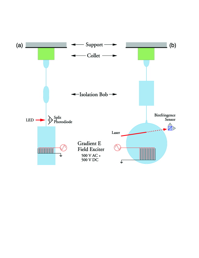
Figure 1: (a) The suspended microscope slide and exciter.  (b) The suspended disk and exciter. In both (a) and (b), the entire structure below the steel collet is fused silica.

In order to reduce systematic errors in the $Q$ measurements, we took a number of steps to reduce excess loss (technical sources of loss, extrinsic to the sample) YingleiPaper ; Gretarsson . All the $Q$’s were measured in a vacuum space pumped down to at least $1\times 10^{-5}$ torr, and more typically $2\times 10^{-6}$ torr. This reduced mechanical loss from gas damping. During the $Q$ measurements, the samples were hung below a monolithic silica suspension made by alternating a massive bob of silica with thin, compliant, silica fibers. The suspensions and samples are shown in Fig. 1. (The suspension is of the same style used previously in highq , Gretarsson , and amaldi .) The piece of fused silica rod at the top of the suspension is held in a collet which is rigidly connected to the underside of a thick aluminum plate supported by three aluminum columns. Between the piece of rod held in the collet and the sample was a single fused silica isolation bob. Its function was to stop vibrations from traveling between the sample and the aluminum optical table from which it was suspended. The size chosen for the isolation bob depended on the sample, with the heavier sample requiring a larger bob. The two fibers in the suspension were monolithically pulled out of the neighboring parts using a H₂-O₂ torch. These fibers had a typical diameter of roughly 100-200 $\mu$m. The normal modes of the sample were excited using a comb capacitor Cadez . This exciter was made from two copper wires sheathed with Teflon, each having a total diameter of about 1/2 mm. The two wires were then wrapped around a ground plane and placed about 1 mm from the face of the sample. Special care was taken to ensure that the exciter and the sample did not touch at any point. The position of the exciter is shown in Fig 1. Alternating wires of the comb capacitor were given a 500 V DC voltage while the other wires were held at ground to induce a polarization in the glass sample. To reduce any eddy current damping YingleiPaper and to reduce the probability that polarized dust could span the gap between the sample and the exciter, the exciter was always kept more than 1/2 mm away from the sample. An AC voltage at a resonance frequency of the sample was then added to the DC voltage to excite the corresponding mode. Once the mode had been excited (“rung up”) to an amplitude where it could be seen clearly above the noise, both the AC and DC voltages were removed and both exciter wires were held at ground. The sample was then allowed to ring down freely.

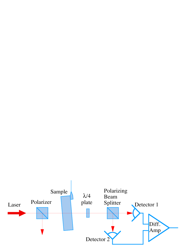
Figure 3: Layout of the birefringence sensor.

The amplitude of excitation in the sample was read out using a birefringence sensor Startin ; AA or (in the earliest measurements) by a shadow sensor. For the birefringence sensor, a linearly polarized beam is passed through the sample at or near a node of the resonant mode under study. Modally generated stress at the node induces birefringence in the glass, which couples a small amount of the light into the orthogonal polarization, phase shifted by $\pi/2$. Thus, the light exiting the sample is slightly elliptically polarized. The beam is then passed through a $\lambda/4$ wave-plate aligned with the initial polarization. This brings the phases of the two orthogonal polarization components together, converting the elliptically polarized light to a linear polarization that is rotated slightly compared with the initial polarization. The rotation angle is (to first order) proportional to the modal strain, and is measured by splitting the beam with a polarizing beamsplitter and monitoring the relative intensity of light in the two channels. This was done with two identical photodiodes and a differencing current-to-voltage amplifier. The output voltage oscillates sinusoidally at the resonant frequency in proportion to the modally induced strain. This signal is sent to a lock-in amplifier to demodulate it to a lower frequency, and the data is collected on a PC. The ringdown time $\tau_{n}$ was obtained by fitting the acquired signal to a damped sinusoid, or by extracting the envelope of the decay. Both approaches yielded the same results, although the accuracy of the former was less sensitive to corruption from noise. A schematic drawing of the optical readout system is shown in Fig. 3.

For the shadow sensor, an LED is used to cast the shadow of the fused silica suspension fiber onto a split photodiode. The LED/diode pair is positioned close to where the suspension fiber is welded to the edge of the sample. The fiber near the weld point will faithfully follow the motion of the edge of the sample. As the sample resonates, the fiber’s shadow moves back and forth on the photodiode at the same frequency. The amount of light falling on each half of the split photodiode changes proportionally. The currents from each half of the photodiode are then compared with a differential current-to-voltage amplifier as in the case of the birefringence sensor. The data acquisition and analysis were identical for both sensors.

For relatively rigid but transparent samples like the ones used here, the birefringence sensor is significantly more sensitive and much easier to use than the shadow sensor. The shadow sensor is better suited to more compliant samples. In both cases however, the dominant sources of broadband noise were laser noise and noise from the differential amplifier.

The samples were coated by Research Electro-Optics Corporation (REO) of Boulder, Colorado, USA. The coating was a dielectric optical coating consisting of alternating layers of SiO₂ and Ta₂O₅. The coating was laid down using Argon ion beam sputtering, followed by annealing at 450^∘C. We chose to examine this particular type of coating because it is the one used on the initial LIGO mirrors that are currently installed at the LIGO sites. This coating is also the type currently proposed for advanced LIGO optics.

The first samples we studied were three rectangular prisms in the shape of microscope slides (7.6 cm $\times$ 2.5 cm $\times$ 0.1 cm) made of Suprasil 2 brand fused silica from Heraeus Quartzglas GmbH of Hannau, Germany. The surface of these samples was treated with a commercial polish to a scratch/dig specification of 80/50. There was no specification on the overall flatness or the surface figure. Two of the three slides (Slide A and Slide B) were coated on both sides with a reflective $\mathrm{Ta_{2}O_{5}}$/$\mathrm{SiO_{2}}$ coating of 3% transmittance for normally incident, $1~{}\mu\mathrm{m}$ wavelength light. The third slide (Slide C) was left uncoated as a control. Slide A was suspended from a corner, which had remained uncoated due to being supported at those points during coating. Therefore, welding the suspension fiber to the corner did not induce visible damage to the coating. Slide B on the other hand was suspended from the center of one of its short edges. During the weld, the coating near the suspension point was visibly damaged in a small crescent shaped of radius  2 mm surrounding the suspension point. This damaged region was etched off using hydrofluoric (HF) acid. Table 1 shows the modes and quality factors for which $Q$’s were repeatably measured. A preliminary version of these results was reported at the Third Edoardo Amaldi Conference On Gravitational Waves amaldi .

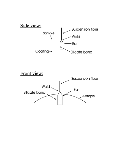
Figure 2: Details of the attachment point. The suspension fiber is welded to the top of the ear. The ear is in turn silicate bonded along one of its flat faces to the uncoated side of the sample.

After measuring the $Q$’s of the slides, we obtained from Zygo Corporation of Middlefield Connecticut a disk of Dynasil brand fused silica, 164.85 mm in diameter and 19.00 mm thick. In an effort to determine the effect of surface preparation on the loss due to optical coatings, this sample was made with strict specification on surface flatness, scratch/dig, and surface roughness. The coated surface had a surface flatness less than $\lambda/20$ ($\lambda=633~{}\mathrm{nm}$), a scratch/dig of 60/40, and a surface roughness less than $4$ Å rms. The back surface had a surface flatness less than $\lambda/6$, a scratch/dig of 60/40, and a surface roughness less than $4$ Å rms. These specifications are nearly as stringent as the actual requirements for LIGO mirrors. To avoid destroying the surface with welding, an “ear” of fused silica was bonded onto the back surface using hydroxy catalysis bonding (silicate bonding) silicatebond . This ear is shaped like a rectangular block with a pyramid on one face. One face of the block is bonded to the sample, so that the tip of the pyramid faces radially. This allows the monolithic suspension to be welded with a torch to the tip of the pyramid without heating the sample very much. See Fig. 2. Once hung, the $Q$ of the sample was measured using the birefringence readout.

Due to the thickness of this sample (required to meet the flatness specification), only one normal mode had a frequency below 5 kHz. The useful bandwidth of the high voltage amplifier that was used to drive the exciter is about 5 kHz, so measurements were possible only on this mode. This was the “butterfly” mode, with two radial nodal lines ($\ell=2$) and no circumferential nodal lines (n=0) Blevins .

After measuring the $Q$ of this uncoated sample, it was sent to REO to be coated. It received a high reflective (HR) coating on one side having 1 ppm transmittance and optimized for a $45^{\circ}$ angle of incidence. The sample was then rehung and the $Q$ remeasured. As can be seen from Table 2, the coating caused a significant reduction in the quality factor. To rule out possible excess loss due to the suspension, the sample was then removed and again rehung. During this hanging attempt (between successful hangings numbers 3 and 4 in Table 2), the isolation bob fell and sheared off the bonded ear. The bond did not give; rather, material from the sample pulled out along with the ear. A second ear was re-bonded at 180^∘ to the original ear. Unfortunately, this ear was also sheared off in the same way during the attempt to suspend the sample. This time the source of the break occurred along the bonded surface, although some of the substrate pulled away as well. Finally, a third attempt succeeded with an ear bonded at $90^{\circ}$ to the original ear (hanging number 4 in Table 2). Despite the broken ears, the quality factor of the coated disk did not change significantly. The results of all $Q$ measurements on the disk are shown in Table 2.

Since it is difficult in any measurement of high $Q$’s to completely eliminate the extrinsic, technical sources of loss (excess loss), the quality factors measured for a given sample varied slightly from mode to mode or within a single mode between different hangings. Since excess loss always acts to reduce the measured $Q$, the best indicator of the true internal friction of a sample is the quality factor of the highest $Q$ mode over all modes and hangings. The spread of measured $Q$’s within single hangings was relatively small. For example, the three $Q$’s measured in hanging number two (sample uncoated) were all between $3.1\times 10^{6}$ and $2.8\times 10^{6}$. The twelve $Q$’s measured in hanging three (sample coated) were all within $1.28\times 10^{6}$ to $1.09\times 10^{6}$. As can be seen from Tables 1 and 2, the measured $Q$’s also did not vary much between modes or hangings, nor between samples in the case of the two coated slides. The reproducibility of the $Q$’s of the disk argues strongly that neither the silicate-bonded ear nor the broken ears affected the loss of the sample. The range of measured $Q$’s for nominally similar situations is indicative of the level of the variable excess loss. Thus, for all our samples, the large difference in $Q$ between the coated and the uncoated measurements must be due to the coating, and not to statistical variation, excess loss, nor, in the case of the disk, to the broken ears.

IV Results

Using the procedure described in Sec. III, we obtained $Q$ values from both the slides and the thick disk. To calculate $\phi_{\|}$ from the measured $Q$’s we need to know the value of $\delta\tilde{U}_{\|}\,d/U$ for each measured mode of the samples. For transverse bending of the slides, the strain is approximately

$$\epsilon_{ij}(\vec{r})=\left\{\begin{array}[]{cl}\frac{\partial^{2}u_{y}(z)}{\partial z^{2}}\,y&\quad i=j=z\\ 0&\quad\mbox{otherwise}\\ \end{array}\right.$$ (30)

where $z$ is the coordinate in the slides’ longest dimension, $y$ is the coordinate in the slides’ shortest dimension with the origin in the center plane of the slide, and $u_{y}(z)$ is the transverse displacement of the center plane of the slides due to the bending. Displacements in directions other than $y$ are zero for the transverse bending modes. This gives

$$\left[\frac{\delta\tilde{U}_{\|}\,d}{\tilde{U}}\right]_{\mathrm{slide}}=7.2\times 10^{-3}$$ (31)

for all transverse bending modes of the slides. The butterfly mode of the disk is more complex, and an analytical expression for strain amplitude $\epsilon(\vec{r})$ was not found. We made an FEA model of this sample and calculated $U_{\mathrm{coating}}/U$ numerically. This resulted in a value of

$$\left[\frac{\delta\tilde{U}_{\|}\,d}{\tilde{U}}\right]_{\mathrm{disk}}\approx\;\left[\frac{U_{\mathrm{coating}}}{U}\right]_{\mathrm{disk}}=5.3\times 10^{-3}$$ (32)

for the butterfly mode of the disk.

The quantities needed to calculate $\phi_{\mathrm{coated}}$ from Eq. (27) are shown in Table 3. Substituting the $Q$ measurements from Table 1 into Eq. (26) to get the loss angles, then using Eq. (31) and the values in Table 3 in Eq. (27) and solving for $\phi_{\|}$, we get

$$\phi_{\|,\mathrm{slide}}=4.2\pm 0.3\times 10^{-4}.$$ (33)

Similarly, from Eq. (32) and the disk $Q$’s in Table 2 we get

$$\phi_{\|,\mathrm{disk}}=1.0\pm 0.3\times 10^{-4}.$$ (34)

The agreement in order of magnitude between these two measured values for $\phi_{\|}$ sets a scale for coating thermal noise. This allows us to make rough estimates of the effect of coating thermal noise on advanced LIGO. The value of $\phi_{\|}$ for the polished disk agrees within its uncertainty with the value measured for coating loss by the Glasgow/Stanford experiment glasgowcoating , despite the use of a different coating material in that experiment ($\mathrm{Ta_{2}O_{5}}$/Al₂O₃ as opposed to Ta₂O₅/$\mathrm{SiO_{2}}$). This suggests that the substrate surface-polish, which is of similar quality on the disk and on the Glasgow/Stanford samples but less good on the slides, may be an important factor contributing to the loss. Further tests and comparisons are necessary before definitive conclusions can be drawn on this issue.

V Implications

Using Eq. (24) for the thermal noise due to the coated mirrors, we can now estimate the thermal noise spectrum of the advanced LIGO interferometer. We calculated the range of coating thermal noise in the pessimistic case using the $\phi_{\|}=4\times 10^{-4}$ (from the slide results) and in the more optimistic case using $\phi_{\|}=1\times 10^{-4}$ (from the disk result). In both cases, we assumed a beam spot size of 5.5 cm, which is the maximum obtainable on fused silica when limited by thermal lensing effects SystemsDesignDocument . We have extrapolated our results to sapphire substrates using the known material properties of sapphire, even though we didn’t measure coating loss directly on sapphire. (There have been recent measurements of $\phi_{\|}$ for REO coatings deposited on sapphire sheilatalk . Those results are in rough agreement with the measurements described here.) As mentioned before, the thermal noise estimates will be least accurate for sapphire substrates because sapphire coating thermal noise is likely to be dominated by $\phi_{\perp}$ which has not been measured. The Young’s modulus of sapphire is considerably higher than both Ta₂O₅ and SiO₂ in bulk, so it seems likely that the coating Young’s modulus is considerably less than sapphire’s. We are aware of a single, preliminary, measurement of $Y^{\prime}$ for a Ta₂O₅/SiO₂ coating Nazario which suggests that the Young’s modulus of the coating is roughly equal to that of fused silica. We know of no measurements of the coating’s Poisson ratio. For the purposes of estimating coating thermal noise, we will set the Young’s modulus and Poisson ratio of the coating equal to that of fused silica.

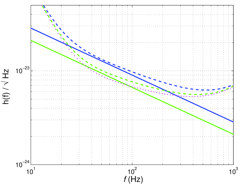
Figure 4: Strain spectrum for advanced LIGO with fused silica mirrors. The solid, straight lines represent the test mass thermal noise; the dashed curves show the total interferometer noise. The lighter curves were generated using optimistic assumptions including $\phi_{\|}=1\times 10^{-4}$. The darker curves were generated using pessimistic assumptions including $\phi_{\|}=4\times 10^{-4}$. The curve shown with dotted lines is the advanced LIGO noise curve without coating noise as modeled in the Advanced LIGO System Design document. In each case, the parameters have been optimized for binary neutron star inspiral.

Table 4 compares the thermal noise estimates for the four cases considered (optimistic estimates and pessimistic estimates on both fused silica and sapphire substrates) to the thermal noise estimates when coatings are not taken into account. The corresponding noise spectra for advanced LIGO are shown in Figs. 4 and 5. These were generated using the program BENCH 1.13 bench and show both the total noise and the contribution from the test mass thermal noise. The curves for the total noise were generated using the noise models and parameters from the advanced LIGO systems design document SystemsDesignDocument . The figures show that coating thermal noise is a significant source of noise in the frequency band $\sim$ 30–400 Hz for fused silica test masses and $\sim$ 40–500 Hz for sapphire test masses.

These estimates are only preliminary indications of the level of coating induced thermal noise. The largest source of uncertainty in these thermal noise estimates is that no measurement has been made of $\phi_{\perp}$. Also, the Young’s modulus of the coating material has not been definitively measured. The half-infinite test mass approximation adds extra uncertainty and this estimate needs to be refined by taking the finite size of the coated test mass into account. In addition, there remains the possibility that the loss associated with the different terms in the energy density $\rho_{\|}$ are not equal as supposed here. However, if this were the case, the apparent consistency of the loss between different modes of the samples measured at Glasgow and Stanford glasgowcoating would be spurious.

We have also examined the effect of coating thermal noise on the expected sensitivity of the initial LIGO interferometers that are currently being commissioned. In initial LIGO, shot noise will be greater than in advanced LIGO and seismic noise will be significant up to about 40 Hz. Due to the higher level of these other noise sources, test mass thermal noise was not expected to be a large contributor to the total noise Abramovici . The addition of coating thermal noise raises the overall noise in the most sensitive frequency band, around 200 Hz, by only 4% . Thus, coating thermal noise should not significantly impact the sensitivity of initial LIGO.

In addition to the interferometers used for gravitational wave detection, there are a number of prototype interferometer within the gravitational wave community. We have examined data from one of these — the 40 m prototype located at Caltech 40m . In this interferometer, the beam spot size was 0.22 cm and the highest $Q$ seen for a mirror mode was $Q_{\mathrm{max}}=8.1\times 10^{6}$ GillespieRaab . Using Eq. (24) with $\phi_{\|}=\phi_{\perp}=1\times 10^{-4}$ and $\phi_{\mathrm{substrate}}=1/Q_{\mathrm{max}}$ in Eq. (24) yields a predicted thermal noise of $\sim 2\times 10^{-19}$ m/$\sqrt{\mathrm{Hz}}$ at 300 Hz. This is consistent with Fig. 3 of 40m . Coating thermal noise is therefore a possible explanation for the broadband excess noise seen between 300 Hz and 700 Hz. The effect of coating thermal noise is also being explored in the Glasgow 10 meter prototype, the Thermal Noise Interferometer (TNI) at Caltech Libbrecht and in the LASTI prototype at MIT.

VI Future work

The measurements and predictions described here indicate that mechanical loss associated with dielectric optical coatings may be a significant source of thermal noise in advanced LIGO. Plans are underway for experiments that will allow us to better understand and, perhaps, reduce the coating thermal noise. A program of loss measurements on various optical coatings deposited on both fused silica and sapphire substrates has begun so that the most appropriate coating may be found. There are also plans to try and correlate the loss angle of the coating with other methods of interrogating its structure. To improve the coating thermal noise without major changes to the optics, the coating loss must be reduced. Study of different dielectric materials is clearly warranted, and changes in the deposition process or post-deposition annealing might also lead to improvements. An agreement has been reached between the LIGO laboratory and two optical coating companies to engage in such research.

Two main models exist for understanding the source of the excess loss in the coating. One is that the internal friction of the coating materials, thin layers of Ta₂O₅ and SiO₂, is high. The other model is that the excess damping comes from rubbing between the layers, and between the coating and the substrate. Experiments are underway to test these models.

Measurement of the unknown parameters in Eq. (22) are crucial. As discussed in Sec. II, ringdown $Q$ measurements can not determine $\phi_{\perp}$ due to the boundary conditions on the free vibration of a sample. A variation of the anelastic aftereffect experiment AA , which will measure the relaxation rate of the coating after being stressed perpendicularly to the substrate, is being pursued at Caltech Willems . This experiment should give a direct measurement of $\phi_{\perp}$.

As seen in Eq. (22), the coating thermal noise in an interferometer is a strong function of the laser spot size. Increasing the size of the laser spot reduces the effect of the coating loss on the total thermal noise, so large spot sizes are desirable. Large spots also help decrease the effect of thermoelastic damping in sapphire mirrors Braginsky , so configurations to increase the spot size are already being considered. A spot size of about 6 cm is the largest that can be achieved on the 25 cm diameter test masses while still keeping the power lost due to diffraction below $\sim 15$ ppm. In the case of 25 cm diameter fused silica test masses, the largest spot size that can be achieved is about 5.5 cm, limited by thermal lensing SystemsDesignDocument . Larger diameter test masses and correspondingly larger spot sizes would be one way to reduce the effects of the coating loss on advanced LIGO’s noise. However, this would require a re-evaluation of a number of advanced LIGO subsystems.

Appendix A Stresses and strains in the coating

We obtain the stresses and strains in the coating in terms of the stresses and strains in the surface of the substrate by utilizing the thin coating approximation, and assuming that the coating Poisson’s ratio is not very different from that of the substrate. Denoting strains by $\epsilon_{ij}$ and stresses by $\sigma_{ij}$, this can be summarized in terms of the following constraints. In cylindrical coordinates,

$$\left.\begin{array}[]{lll}&\epsilon_{rr}^{\prime}&=\epsilon_{rr}\\ &\epsilon_{\theta\theta}^{\prime}&=\epsilon_{\theta\theta}\\ &\epsilon_{rz}^{\prime}&=\epsilon_{rz}\\ &\sigma_{zz}^{\prime}&=\sigma_{zz}\\ &\sigma_{rz}^{\prime}&=\sigma_{rz}\end{array}\right.$$ (35)

where primed quantities refer to the coating and the unprimed quantities refer to the surface of the substrate. Due to axial symmetry $\epsilon_{r\theta}^{\prime}=\epsilon_{z\theta}^{\prime}=\sigma_{r\theta}^{\prime}=\sigma_{z\theta}^{\prime}=0$. We use the following relations, valid for axially symmetric deformations Bondu

$$\left.\begin{array}[]{lll}\sigma_{rr}&=&(\lambda+2\mu)\epsilon_{rr}+\lambda\epsilon_{\theta\theta}+\lambda\epsilon_{zz}\\ \sigma_{\theta\theta}&=&\lambda\epsilon_{rr}+(\lambda+2\mu)\epsilon_{\theta\theta}+\lambda\epsilon_{zz}\\ \sigma_{zz}&=&\lambda\epsilon_{rr}+\lambda\epsilon_{\theta\theta}+(\lambda+2\mu)\epsilon_{zz}\\ \sigma_{rz}&=&2\mu\epsilon_{rz}\end{array}\right.$$ (36)

where $\lambda$ and $\mu$ are the Lamé coefficients. In terms of Young’s modulus and Poisson’s ratio, the Lamé coefficients are

$$\begin{array}[]{lll}\lambda&=&Y\sigma/((1+\sigma)(1-2\sigma)),\\ \mu&=&Y/(2(1+\sigma)).\end{array}$$ (37)

Combining Eqs. (35) and Eqs. (36), we obtain the stresses and strains in the coating in terms of the stresses and strains in the surface of the substrate

$$\left.\begin{array}[]{lll}\epsilon_{rr}^{\prime}&=&\epsilon_{rr}\\ \epsilon_{\theta\theta}^{\prime}&=&\epsilon_{\theta\theta}\\ \epsilon_{zz}^{\prime}&=&\frac{\lambda-\lambda^{\prime}}{\lambda^{\prime}+2\mu^{\prime}}\,(\epsilon_{rr}+\epsilon_{\theta\theta})+\frac{\lambda+2\mu}{\lambda^{\prime}+2\mu^{\prime}}\,\epsilon_{zz}\\ \epsilon_{rz}^{\prime}&=&\epsilon_{rz}\\ \sigma_{rr}^{\prime}&=&(\lambda^{\prime}+2\mu^{\prime})\epsilon_{rr}+\lambda^{\prime}\epsilon_{\theta\theta}+\lambda^{\prime}\epsilon_{zz}^{\prime}\\ \sigma_{\theta\theta}^{\prime}&=&\lambda^{\prime}\epsilon_{rr}+(\lambda^{\prime}+2\mu^{\prime})\epsilon_{\theta\theta}+\lambda^{\prime}\epsilon_{zz}^{\prime}\\ \sigma_{zz}^{\prime}&=&\sigma_{zz}\\ \sigma_{rz}^{\prime}&=&\sigma_{rz}\end{array}\right.$$ (38)

where $\lambda^{\prime}$ and $\mu^{\prime}$ are the Lamé coefficients of the coating, and $\lambda$ and $\mu$ are the Lamé coefficients of the substrate.

We obtain the stresses and strains in the substrate $\epsilon_{ij}$, $\sigma_{ij}$ from the general solutions to the axially symmetric equations of elasticity for an infinite half-space Bondu ; ThorneLiu

$$\begin{array}[]{lll}u_{r}(r,z)&=&\int_{0}^{\infty}\,[\alpha(k)-\frac{\lambda+2\mu}{\lambda+\mu}\,\beta(k)+\beta(k)kz]\,e^{-kz}\!J_{1}(kr)\,kdk\\ u_{z}(r,z)&=&\int_{0}^{\infty}\,[\alpha(k)+\frac{\mu}{\lambda+\mu}\,\beta(k)+\beta(k)kz]\,e^{-kz}\!J_{0}(kr)\,kdk\\ u_{\theta}(r,z)&=&0\qquad\mbox{(Axial symmetry)},\end{array}$$ (39)

where $u_{r}(r,z)$ is the radial deformation of the test mass, $u_{z}(r,z)$ is the deformation of the test mass perpendicularly to the face ($z$ being positive inward), and $u_{\theta}(r,z)$ is the transverse displacement. $J_{1}(kz)$ and $J_{0}(kz)$ are Bessel functions of the first kind. The functions $\alpha(k)$ and $\beta(k)$ are determined by the boundary conditions at the front face: $\sigma_{rz}(r,z=0)=0$ and $\sigma_{zz}(r,z=0)=p(r)$ Bondu . Using the pressure distribution $p(r)$ from Eq. (8) gives

$$\alpha(k)=\beta(k)=\frac{F}{4\pi\mu\,k}\,\exp\left(-\frac{1}{8}\,k^{2}w^{2}\right).$$ (40)

Substituting Eq. (40) into Eqs. (39) and performing the integrals leads to

$$u_{r}(r,z=0) = -\frac{F(\omega)}{4\pi(\lambda+\mu)r}\left[1-\exp\!\left(-\frac{2r^{2}}{w^{2}}\right)\right],$$ (41)

$$u_{z}(r,z=0) = \frac{F(\omega)\,(\lambda+2\mu)}{2\sqrt{2\pi}\,(\lambda+\mu)\mu w}\;\exp\!\left(-\frac{r^{2}}{w^{2}}\right)I_{0}\!\left(\frac{r^{2}}{w^{2}}\right)$$ (42)

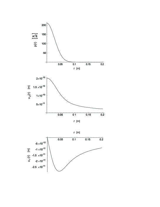
Figure 6: Top: Pressure distribution $p(r)$ from Eq. (8) (with $F$ set to unity). The pressure distribution has the same shape as the laser intensity.  Center: The resulting response of the surface in the axial direction, $u_{z}(r)$. The impression is wider than the applied pressure.  Bottom: The resulting response in the radial direction, $u_{r}(r)$. As expected, the surface is pulled toward the center.

where $I_{0}$ is a modified Bessel function of the first kind. These deformations are shown, along with the pressure distribution $p(r)$, in Fig. 6. The strains in the substrate are obtained from the relations

$$\begin{array}[]{lll}\epsilon_{rr}&=&\delta u_{r}/\delta r\\ \epsilon_{\theta\theta}&=&u_{r}/r\\ \epsilon_{zz}&=&\delta u_{z}/\delta z\\ \epsilon_{rz}&=&(\delta u_{z}/\delta r+\delta u_{r}/\delta z)/2.\end{array}$$ (43)

These strains can now be used to find the stresses in the surface of the substrate through Eqs. (36), and then to find the stresses and strains in the coating through Eqs. (38). The results for the surface of the substrate are

$$\begin{array}[]{lll}\epsilon_{rr}&=&\frac{F}{4\pi(\lambda+\mu)}\left(\frac{1}{r^{2}}\left(1-e^{-2r^{2}/w^{2}}\right)-\frac{4}{w^{2}}\,e^{-2r^{2}/w^{2}}\right)\\ \epsilon_{\theta\theta}&=&-\frac{F}{4\pi(\lambda+\mu)}\left(\frac{1}{r^{2}}\left(1-e^{-2r^{2}/w^{2}}\right)\right)\\ \epsilon_{zz}&=&-\frac{F}{4\pi(\lambda+\mu)}\left(\frac{4}{w^{2}}\,e^{-2r^{2}/w^{2}}\right)\\ \epsilon_{rz}&=&0\\ \sigma_{rr}&=&\frac{F}{2\pi(\lambda+\mu)}\left(\frac{\mu}{r^{2}}\left(1-e^{-2r^{2}/w^{2}}\right)-\frac{4(\lambda+\mu)}{w^{2}}\,e^{-2r^{2}/w^{2}}\right)\\ \sigma_{\theta\theta}&=&-\frac{F}{2\pi(\lambda+\mu)}\left(\frac{\mu}{r^{2}}\left(1-e^{-2r^{2}/w^{2}}\right)+\frac{4\lambda}{w^{2}}\,e^{-2r^{2}/w^{2}}\right)\\ \sigma_{zz}&=&-\frac{F}{2\pi}\,\left(\frac{4}{w^{2}}\,e^{-2r^{2}/w^{2}}\right)\\ \sigma_{rz}&=&0\\ \end{array}$$ (44)

and for the coating

$$\begin{array}[]{lll}\epsilon_{rr}^{\prime}&=&\epsilon_{rr}\\ \epsilon_{\theta\theta}^{\prime}&=&\epsilon_{\theta\theta}\\ \epsilon_{zz}^{\prime}&=&-\frac{F(2(\lambda+\mu)-\lambda^{\prime})}{4\pi(\lambda+\mu)(\lambda^{\prime}+2\mu^{\prime})}\left(\frac{4}{w^{2}}\,e^{-2r^{2}/w^{2}}\right)\\ \epsilon_{rz}^{\prime}&=&0\\ \sigma_{rr}^{\prime}&=&\frac{F}{2\pi(\lambda+\mu)(\lambda^{\prime}+2\mu^{\prime})}\left(\frac{\mu^{\prime}(\lambda^{\prime}+2\mu^{\prime})}{r^{2}}\left(1-e^{-2r^{2}/w^{2}}\right)-\frac{4(\lambda^{\prime}(\lambda+\mu)+2\mu^{\prime}(\lambda^{\prime}+\mu^{\prime}))}{w^{2}}\,e^{-2r^{2}/w^{2}}\right)\\ \sigma_{\theta\theta}^{\prime}&=&-\frac{F}{2\pi(\lambda+\mu)(\lambda^{\prime}+2\mu^{\prime})}\left(\frac{\mu^{\prime}(\lambda^{\prime}+2\mu^{\prime})}{r^{2}}\left(1-e^{-2r^{2}/w^{2}}\right)+\frac{4(\lambda^{\prime}(\lambda+\mu+\mu^{\prime}))}{w^{2}}\,e^{-2r^{2}/w^{2}}\right)\\ \sigma_{zz}^{\prime}&=&\sigma_{zz}\\ \sigma_{rz}^{\prime}&=&0\,.\end{array}$$ (45)

Equations (44) can now be used to find the energy density in the substrate and integrated over the half-infinite volume, Eq. (16), to give the total energy in the substrate, Eq. (17). Equations (45) can be substituted into the expression for the energy density at the surface, Eq. (13), and integrated over the surface to give the expressions for $\delta U_{\|}$ and $\delta U_{\bot}$ in Eqs. (18) and (19).

Slide	Coating	Mode	Frequency	Q
A	HR	2	1022 Hz	$1.1\pm 0.5\times 10^{5}$
	HR	3	1944 Hz	$1.6\pm 0.1\times 10^{5}$
	HR	4	2815 Hz	$1.6\pm 0.1\times 10^{5}$
B	HR	2	962 Hz	$1.3\pm 0.1\times 10^{5}$
C	none	2	1188 Hz	$4.0\pm 0.2\times 10^{6}$
	none	3	2271 Hz	$4.9\pm 0.3\times 10^{6}$

Table 1: Measured $Q$’s for transverse bending modes of the three commercially polished fused silica slides. Slides A and B were coated while slide C was left uncoated as a control.

Hanging Number	Coating	Frequency	Q
1	none	4107 Hz	$3.46\pm 0.02\times 10^{6}$
2	none	4107 Hz	$3.10\pm 0.007\times 10^{6}$
3	HR ($45^{\circ}$)	4108 Hz	$1.28\pm 0.02\times 10^{6}$
4†	HR ($45^{\circ}$)	4121 Hz	$1.24\pm 0.001\times 10^{6}$
†Ear was sheared off twice before this hanging.

Table 2: Measured $Q$’s for butterfly mode of the superpolished fused silica disk. In hangings 1 and 2, the disk remained uncoated whereas in hangings 3 and 4 the disk had been coated.

Sample	Parameter	Value	Units
Slide	Coating Layers	14
	Coating Thickness $d$	2.4	$\!\mu$m
Disk	Coating Layers	38
	Coating Thickness $d$	24.36	$\!\mu$m
Both	Substrate Young’s modulus ($Y$)	$7.0\times 10^{10}$	N/m2
	Coating Young’s modulus ($Y^{\prime}$)	$7\times 10^{10}$	N/m2

Table 3: Physical parameters of the coating and samples. These values are used to calculate the coating loss $\phi_{\|}$ from Eq. (27). The value of the coating Young’s modulus is a preliminary result from SMA/Virgo in Lyon, France.

Test mass		$Q_{\mathrm{eff}}~{}~{}~{}~{}~{}~{}$	Structural thermal noise
material	Coating loss	(=$1/\phi_{\mathrm{readout}}$)	at 100 Hz,  $\sqrt{S_{h}}$
Sapphire	none	$200\times 10^{6}$	$1\times 10^{-24}$
	$\phi_{\|}=1\times 10^{-4}$	$15\times 10^{6}$	$3\times 10^{-24}$
	$\phi_{\|}=4\times 10^{-4}$	$4\times 10^{6}$	$5\times 10^{-24}$
Fused silica	none	$30\times 10^{6}$	$6\times 10^{-24}$
	$\phi_{\|}=1\times 10^{-4}$	$19\times 10^{6}$	$7\times 10^{-24}$
	$\phi_{\|}=4\times 10^{-4}$	$9\times 10^{6}$	$9\times 10^{-24}$

Table 4: Comparison of structural thermal noise with and without taking coatings into account. The effective quality factor $Q_{\mathrm{eff}}$ (equal to the reciprocal of $\phi_{\mathrm{readout}}$) represents the quality factor a homogeneous mirror would need to have to give the same structural contribution to thermal noise as the actual coated mirror. (The effect of thermoelastic damping, important for sapphire, is not included in $Q_{\mathrm{eff}}$). The final column shows the strain amplitude thermal noise at 100 Hz in the advanced LIGO interferometer resulting from structural loss in the test mass coatings and substrates.

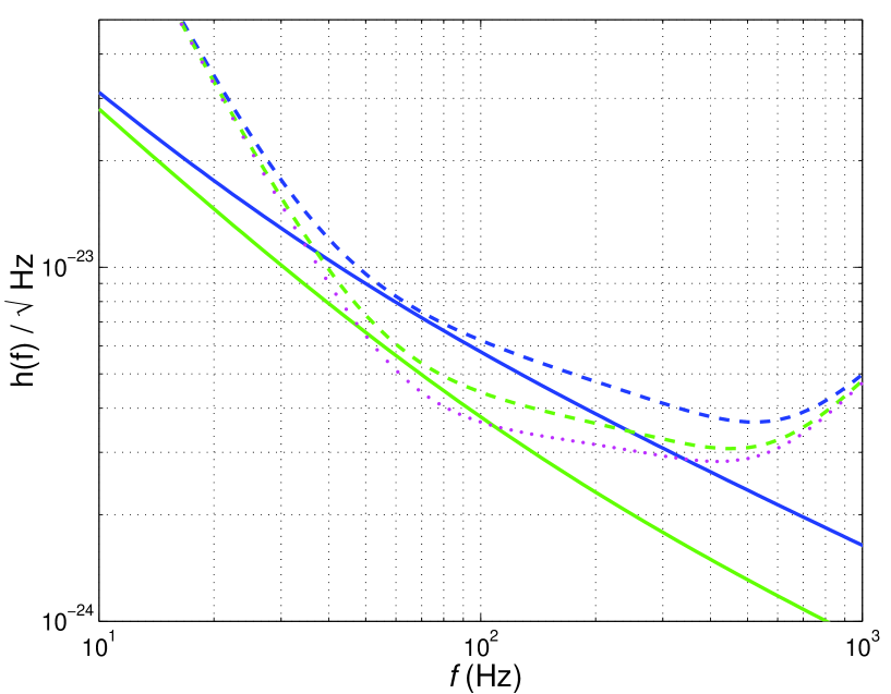
Figure 5: Strain spectrum for advanced LIGO with sapphire mirrors. The solid, straight lines represent the test mass thermal noise; the dashed curves show the total interferometer noise. The lighter curves were generated using optimistic assumptions including $\phi_{\|}=1\times 10^{-4}$. The darker curves were generated using pessimistic assumptions including $\phi_{\|}=4\times 10^{-4}$. The curve shown with dotted lines is the advanced LIGO noise curve without coating noise as modeled in the Advanced LIGO System Design document. In each case, the parameters have been optimized for binary neutron star inspiral.

References

- (1) A. Abramovici et al, Science 256, 325 (1992).
- (2) A. Giazotto, Nucl. Instrum. Meth. A 289, 518 (1988).
- (3) K. Danzmann et al., Max-Planck-Institut für Quantenoptik Report 190, Garching Germany, (1994).
- (4) K. Tsubono, Gravitational Wave Experiments, Proceedings of the First Edoardo Amaldi Conference, 112 (Singapore, World Scientific, 1995).
-
(5)
LSC White Paper on Detector Research and Development
Available at
http://www.ligo.caltech.edu/docs/T/T990080-00.pdf. - (6) Internal report, Max-Planck Institut für Quantenoptik, D-85748 Garching, (2000).
- (7) K. Kuroda et al., Int. J. Mod. Phys. D 8, 557 (1999), http://www.icrr.u-tokyo.ac.jp/gr/LCGT.pdf.
- (8) D. B. Fraser, J. Appl. Phys. 39, 5868 (1968); 41, 6 (1970).
- (9) B. S. Lunin, S. N. Torbin, M. N. Danachevskaya, and I. V. Batov, Moscow State Chemistry Bulletin 35, 24 (1994).
- (10) S. D. Penn, G. M. Harry, A. M. Gretarsson, S. E. Kittelberger, P. R. Saulson, J. J. Schiller, J. R. Smith, and S. O. Swords, Rev. Sci. Instrum. bf 72 3670 (2001). Also available at gr-qc/0009035.
- (11) S. Rowan, G. Cagnoli, P. Sneddon, J. Hough, R. Route, E. K. Gustafson, M. M. Fejer, V. Mitrofanov, Phys. Lett. A. 265, 5 (2000).
- (12) V. B. Braginsky, V. P. Mitrofanov, and V. I. Panov, Systems with small dissipation (The University of Chicago Press, Chicago, 1985).
- (13) S. Whitcomb, in Proceedings of the TAMA International Workshop on Gravitational Wave Detection, K. Tsubono (ed.), (Universal Academy Press, Tokyo, 1996).
- (14) H. B. Callen, R. F. Greene, Phys. Rev. 86, 703 (1952).
- (15) D. Crooks, P. Sneddon, G. Cagnoli, J. Hough, S. Rowan, M. M. Fejer, E. Gustafson, R. Route, N. Nakagawa, D. Coyne, G. M. Harry, and A. M. Gretarsson, Phys. Lett. A, this volume.
- (16) Yu. Levin, Phys. Rev. D 57, 659 (1998).
- (17) Y. T. Liu and K. S. Thorne, Phys. Rev. D 62, 122002 (2000).
- (18) K. Numata, G. B. Bianc, N. Ohishi, A. Sekiya, S. Otsuka, K. Kawabe, M. Ando, K. Tsubono, Phys. Lett. A 276, 37 (2000).
- (19) F. Bondu, P. Hello, J. Vinet, Phys. Lett. A 246, 227 (1998).
- (20) N. Nakagawa, oral presentation at the LIGO Scientific Collaboration meeting (Hanford, Washington, USA, Aug. 13-16, 2001).
- (21) N. Nakagawa, A. M. Gretarsson, E. K. Gustafson, and M. M. Fejer, submitted to Phys. Rev. D, gr-qc/0105046.
- (22) Y. L. Huang and P. R. Saulson, Rev. Sci. Instrum. 69 544 (1998).
- (23) A. M. Gretarsson and G. M. Harry, Rev. Sci. Instr. 70 4081 (1999), physics/9904015. In the referenced article, the more general surface loss parameter is used. For coatings, as we have modeled them here, .
- (24) A. M. Gretarsson, G. M. Harry, S. D. Penn, P. R. Saulson, J. J. Schiller, and W. J. Startin, in proceedings of the Third Edoardo Amaldi Conference on Gravitational Waves, edited by S. Meshkov (American Institute of Physics, Melville, New York, (2000), physics/9911040.
- (25) A. Cadez and A. Abramovici, J. Phys. E:Sci. Instr. 21, 453 (1988).
- (26) W. J. Startin, M. A. Beilby, and P. R. Saulson, Rev. Sci. Instr. 69, 3681 (1998).
- (27) M. A. Beilby, P. R. Saulson, and A. Abramovici, Rev. Sci. Instr. 69, 2539 (1998).
- (28) D. H. Gwo, Proceedings of SPIE–The International Society for Optical Engineering, 3435 136 (1998).
- (29) R. D. Blevins, Formulas for Natural Frequency and Mode Shape, Van Nostrand Reihold, New York, 1979.
- (30) P. Fritschel, Advanced LIGO Systems Design, www.ligo.caltech.edu/docs/T/T010075-0.pdf.
- (31) S. Rowan, oral presentation at Aspen Winter Conference on Gravitational Waves (Aspen, Colorado, USA, Feb. 4-10, 2001).
- (32) N. Morgado, SMA Virgo, (private communication).
- (33) The program BENCH is available at http://gravity.phys.psu.edu/Bench/. Note: The contibution from structural internal thermal noise in BENCH 1.12 was found to be erroneously low by a factor of two. This error has been corrected in versions of BENCH 1.13 (Aug. 2001) and higher.
- (34) A. Abramovici, W. Althouse, J. Camp, D. Durance, J. A. Giaime, A. Gillespie, S. Kawamura, A. Kuhnert, T. Lyons, F. J. Raab, R. L. Savage Jr., D. Shoemaker, L Sievers, R. Spero, R. Vogt, R. Weiss, S. Whitcomb, M. Zucker, Phys. Lett. A 218, 157 (1996).
- (35) A. Gillespie and F. Raab, Phys. Rev. D 52, 577 (1995).
- (36) K. Libbrecht, California Institute of Technology (private communication).
- (37) P. Willems, California Institute of Technology, (private communication).
- (38) V. B. Braginksy, M. L. Gorodetsky, S. P. Vyatchanin, Phys. Lett. A 264 (1999),