R=0 spacetimes and self-dual Lorentzian wormholes

Abstract

A two–parameter family of spherically symmetric, static Lorentzian wormholes is obtained as the general solution of the equation $\rho=\rho_{t}=0$, where $\rho=T_{ij}\;u^{i}u^{j}$, $\rho_{t}=(T_{ij}-{1\over 2}T\,g_{ij})\;u^{i}u^{j}$, and $u^{i}\;u_{i}=-1$. This equation characterizes a class of spacetimes which are “self dual” (in the sense of electrogravity duality). The class includes the Schwarzschild black hole, a family of naked singularities, and a disjoint family of Lorentzian wormholes, all of which have vanishing scalar curvature ($R=0$). Properties of these spacetimes are discussed. Using isotropic coordinates we delineate clearly the domains of parameter space for which wormholes, nakedly singular spacetimes and the Schwarzschild black hole can be obtained. A model for the required “exotic” stress–energy is discussed, and the notion of traversability for the wormholes is also examined.

I Introduction

Traversable Lorentzian wormholes have been in vogue ever since Morris, Thorne and Yurtsever mty:prl88 came up with the exciting possibility of constructing time machine models with these exotic objects. The seminal paper by Morris and Thorne mt:ajp88 demonstrated that the matter required to support such spacetimes necessarily violates the null energy condition. This at first made people rather pessimistic about their existence in the classical world. Semiclassical calculations based on techniques of quantum fields in curved spacetime, as well as an old theorem due to Epstein, Glaser and Yaffe egy:inc , raised hopes about the generation of such spacetimes through quantum stresses. The Casimir effect was put to use by MTY themselves to justify their introduction of such spacetimes as a means of constructing model time machines.

In the last twelve years or so there have been innumerable attempts at solving the so-called “exotic matter problem” in wormhole physics. (For a detailed account of wormhole physics up to 1995 see the book by Visser visser:book . For a slightly later survey see geometric .) Alternative theories of gravity alt:prd , evolving (dynamic, time–dependent) wormhole spacetimes sk:prd ; mv:prd ; hochberg with varying definitions of the throat have been tried out as possible avenues of resolution.

Despite multiple efforts, all these spacetimes still remain in the domain of fiction. At times, their simplicity makes us believe that they just might exist in nature though we are very far from actually seeing them in the real world of astrophysics. (For attempts towards astrophysical consequences see ms:01 .)

This paper does not set out to solve the exotic matter problem. On the contrary, it does have exotic matter as the source once again. The obvious query would therefore be — what is actually new? The first novelty is related to the method of construction. Generally, a wormhole is constructed by imposing the geometrical requirement on spacetime that there exists a throat but no horizon. This is however not couched in terms of an equation restricting the stress-energy.

Perhaps for the first time, we are proposing a specific restriction on the form of the stress-energy that, when solving the Einstein equations, automatically leads to a class of wormhole solutions. The characterization we have in mind for our class of static self-dual wormholes is

$$\rho=\rho_{t}=0,$$ (1)

where $\rho$ and $\rho_{t}$ are respectively the energy density measured by a static observer and the convergence density felt by a timelike congruence. (Applying both of these conditions, plus the Einstein equations, implies $R=0$). It is remarkable that the general solution nkd:cs of this equation automatically incorporates the basic characteristics of a Lorentzian wormhole. A generic wormhole spacetime is an ad hoc construction and hence no equation would be able to encompass all wormhole spacetimes. Equation (1) indicates that space is empty relative to timelike particles as they encounter neither energy density nor geodesic convergence. This, in turn, leads to the fact that the general spacetime will be a modification of the Schwarzschild solution, which would be contained in the general solution of equation (1) as a special case. Portions of the general solution space are interpreted as wormhole spacetimes with the throat given by the well known Schwarzschild radius, which no longer defines the horizon. Indeed equation (1) uniquely characterizes a class of “self dual” static wormhole spacetimes which contains the Schwarzschild solution. The notion of duality we have in mind involves the interchange of the active and passive electric parts of the Riemann tensor (termed as electrogravity duality). This duality, which leaves the vacuum Einstein equation invariant, was defined by one of the present authors in nkd:98 . Electrogravity duality essentially implies the interchange of the Ricci and Einstein tensors. For vanishing Ricci scalar, these two tensors become equal and the corresponding solutions could therefore be called self-dual in this sense. Under the duality transformation, $\rho$ and $\rho_{t}$ are interchanged indicating invariance of equation (1). Since energy densities vanish and yet the spacetime is not entirely empty, the matter distribution would naturally have to be exotic (violating all the energy conditions visser:book ). Physically, the existence of such spacetimes might be doubted because of this violation of the weak and null energy conditions. Analogous to the spatial–Schwarzschild wormhole, for which $g_{00}=-1$ and $g_{11}=({1-\frac{2m}{r}})^{-1}$, these spacetimes have zero energy density but nonzero pressures. The spatial–Schwarzschild wormhole is one specific particular solution of the equations $\rho=0$, $\rho_{t}=0$, while here we exhibit the most general solution nkd:cs .

Furthermore, on rewriting the line element in terms of isotropic coordinates we realise the existence of all three classes of spherically symmetric spacetimes — namely the black holes, the wormholes and the nakedly singular geometries — all within the framework of our general solution. This happens through the understanding of the nature of the spacetime for different domains of the two parameters $\kappa$ and $\lambda$ defined below. A detailed discussion on this is included too.

The following section (II) deals with all the above mentioned aspects of $R=0$ spacetimes. In the last section (III) we offer our conclusions and remarks. We choose the metric signature as $(-+++)$ and set $c=1$ unless otherwise stated.

II $R=0$ characterization of Lorentzian wormholes

The Lorentzian wormhole, a la Morris and Thorne, is defined through the specification of two arbitrary functions $b(r)$ and $\phi(r)$ which appear in the following generic version of a spherically symmetric, static line element:

$$ds^{2}=-e^{2\phi(r)}{\mathrm{d}}t^{2}+\frac{{\mathrm{d}}r^{2}}{1-\frac{b(r)}{r}}+r^{2}\left({\mathrm{d}}\theta^{2}+\sin^{2}\theta\;{\mathrm{d}}\varphi^{2}\right).$$ (2)

The properties of $b(r)$ and $\phi(r)$ which ‘make’ a wormhole are mt:ajp88 ; visser:book :

1. A no-horizon condition $\rightarrow$ $e^{2\phi}$ has no zeros.
   (The function $\phi(r)$ is called the red–shift function.)

2. A wormhole shape condition $\rightarrow$  $b(r=b_{0})=b_{0}$;
   with $\frac{b(r)}{r}\leq 1$ ($\forall r\geq b_{0}$).
   ($b(r)$ is called the wormhole shape function.)

3. Asymptotic flatness: $\frac{b(r)}{r}\rightarrow 0$ as $r\rightarrow\infty$.

These features provide a minimum set of conditions which lead, through an analysis of the embedding of the spacelike slice in a Euclidean space, to a geometry featuring two asymptotic regions connected by a bridge. Topologically different configurations where we only have one asymptotic region was the origin of the name ‘wormhole’ a la Wheeler. It is well–known mt:ajp88 ; visser:book that these conditions lead to the requirement that the stress-energy which supports the wormhole violates the null energy condition (and even the averaged null energy condition) mv:prd ; hochberg .

Amongst examples, the simplest is of course the spatial-Schwarzschild wormhole defined by the choice $\phi=0$ and $b(r)=2m$. The horizon is (by fiat) gotten rid of simply by choosing $g_{00}=-1$ and the wormhole shape is retained by choosing $b(r)=2m$. This geometry would of course be contained in the general solution of equation (1). Many other examples can be constructed. There is no general principle as such to generate these wormholes — one might just ‘tailor-make’ them according to ones taste. If we demand that the wormhole spacetime must contain the Schwarzschild spacetime, the equation (1) completely and uniquely characterizes it.

II.1 General solution

In order to make a wormhole, we have to specify/determine two functions. Generally one of them is chosen by fiat while the other is determined by implementing some physical condition. In this paper, we have proposed the equation (1) as the equation for wormhole, which would imply $R=0$, and place a constraint on the wormhole shape function. Alternatively, we could choose the shape function and solve for $R=0$. The $R=0$ constraint will be a condition on $b(r)$ and $\phi(r)$ and its derivatives. In an earlier paper skds:prd $\phi(r)$ was chosen and an appropriate $b(r)$ (satisfying wormhole conditions) was obtained as a solution to the $R=0$ constraint. Here, we do the opposite, first demand $\rho=0$ and then solve for $R=0$, which would determine both $\phi$ and $b$. Interestingly, the most general solution of equation (1) automatically incorporates the requirement of existence of a throat without horizon. This is thus a natural characterization of a Lorentzian wormhole.

Defining the diagonal energy momentum tensor components as $T_{00}=\rho(r)$, $T_{11}=\tau(r)$ and $T_{22}=T_{33}=p(r)$ and using the Einstein equations with the assumption of the line element given above we find that:

$$\rho(r) = \frac{1}{8\pi\;G}\;\frac{b^{\prime}}{r^{2}};$$ (3)

$$\tau(r) = \frac{1}{8\pi\;G}\;\left[-\frac{b}{r^{3}}+2\frac{\phi^{\prime}}{r}\left(1-\frac{b}{r}\right)\right];$$ (4)

$$p(r) = \frac{1}{8\pi\;G}\;\left\{\left(1-\frac{b(r)}{r}\right)\left[\phi^{\prime\prime}-\frac{b^{\prime}r-b}{2r(r-b)}\phi^{\prime}+{\phi^{\prime}}^{2}+\frac{\phi^{\prime}}{r}-\frac{b^{\prime}r-b}{2r^{2}(r-b)}\right]\right\}.$$ (5)

(Note that $\tau$ as defined above is simply the radial pressure $p_{r}$, and differs by a minus sign from the conventions in mt:ajp88 ; visser:book . The symbol $p$ is simply the transverse pressure $p_{t}$.) Implementing the condition $\rho=\rho_{t}$ (or, equivalently $R=T=0$) we find the following equation:

$$\xi^{\prime}+\xi^{2}+\left(\frac{2}{r}-\frac{b^{\prime}r-b}{2r(r-b)}\right)\xi=\frac{b^{\prime}}{r(r-b)},$$ (6)

where $\xi=\phi^{\prime}$ and the prime denotes a derivative with respect to $r$. Given $b(r)$ we can solve the above equation to obtain $\phi$. We note that the above equation (with a given $b$) is a nonlinear, first-order ordinary differential equation which is known in mathematics as a Riccati equation. This equation is covariant under fractional linear transformations of the dependent variable [SL(2,R) symmetry]. In principle equation (6) can be thought of as the ‘master’ differential equation for all spherically symmetric, static $R=0$ spacetimes, examples of which include the Schwarzschild and the Reissner–Nordstrom geometries.

Now solving for $\rho=0$ clearly gives $b=\mathrm{constant}=2m$. Then equation (6) simplifies to:

$$\xi^{\prime}+\xi^{2}+\frac{\xi}{r}\left(\frac{2r-3m}{r-2m}\right)=0.$$ (7)

It admits the most general solution given by

$$g_{00}=-\left(\kappa+\lambda\sqrt{1-\frac{2m}{r}}\right)^{2},$$ (8)

where $\kappa$ and $\lambda$ are constants of integration.

Clearly the Schwarzschild geometry is the special solution for which $R_{ij}=0$, to which the general solution reduces when $\kappa=0$. This shows that the Schwarzschild solution is contained in the above general solution. It also contains the spatial-Schwarzschild wormhole with $g_{00}=-1$ when $\lambda=0$. The solution then admits no horizon but there is a wormhole throat at $r=2m$. We thus have a Lorentzian wormhole.

The components of the energy momentum tensor for this geometry turn out to be:

$$\rho = 0;$$ (9)

$$\tau = -\frac{1}{8\pi\;G}\left[\frac{2m\kappa}{r^{3}\left(\kappa+\lambda\sqrt{1-\frac{2m}{r}}\right)}\right];$$ (10)

$$p = \frac{1}{8\pi\;G}\left[\frac{m\kappa}{r^{3}\left(\kappa+\lambda\sqrt{1-\frac{2m}{r}}\right)}\right].$$ (11)

The weak ($\rho\geq 0$, $\rho+\tau\geq 0$, $\rho+p\geq 0$) and null ($\rho+\tau\geq 0$, $\rho+p\geq 0$) energy conditions are both violated. We note that the stress–energy given above satisfies $\rho+\tau=-2p$; which obviously follows from $R=0\quad\Rightarrow\quad T=0$. The violation of the energy condition stems from the violation of the inequality $\rho+\tau\geq 0$. The extent of the violation, caused by the $1/{r^{3}}$ behaviour of the relevant quantity, is large in the vicinity of the throat. One does have a control parameter $\kappa$, which, can be chosen to be very small in order to restrict the amount of violation.

The complete line element for the geometry discussed above is:

$${\mathrm{d}}s^{2}=-\left(\kappa+\lambda\sqrt{1-{2m\over r}}\right)^{2}\;{\mathrm{d}}t^{2}+{{\mathrm{d}}r^{2}\over 1-2m/r}+r^{2}\left({\mathrm{d}}\theta^{2}+\sin^{2}\theta\;{\mathrm{d}}\varphi^{2}\right).$$ (12)

Of course we could also consider the line element below (obtained by replacing $\lambda$ by $-\lambda$), which also has $R=0$.

$${\mathrm{d}}s^{2}=-\left(\kappa-\lambda\sqrt{1-{2m\over r}}\right)^{2}\;{\mathrm{d}}t^{2}+{{\mathrm{d}}r^{2}\over 1-2m/r}+r^{2}\left({\mathrm{d}}\theta^{2}+\sin^{2}\theta\;{\mathrm{d}}\varphi^{2}\right).$$ (13)

Note that these metrics only make sense (by construction) for $r\geq 2m$. So to really make the wormhole explicit we need two coordinate patches, $r_{1}\in(2m,\infty)$, and $r_{2}\in(2m,\infty)$, which we then have to sew together at $r=2m$. (And in this particular case the geometry is smooth across the junction provided we pick the $+$ root on one side and the $-$ root on the other side, in which case there is no thin shell contribution at the junction.) This is not particularly obvious, and to make this a little clearer, it is convenient to go to isotropic coordinates, defined by

$$r=\bar{r}\left(1+{m\over 2\bar{r}}\right)^{2}.$$ (14)

Since the space part of the metric for the general solution [(12) or (13)] is identical to the space part of the Schwarzschild geometry we can use exactly the same transformation for going from curvature coordinates to isotropic coordinates as was used for Schwarzschild itself. Then it is easy to see that

$${\mathrm{d}}s^{2}=-\left\{\kappa+\lambda\left[{1-m/2\bar{r}\over 1+m/2\bar{r}}\right]\right\}^{2}\;{\mathrm{d}}t^{2}+\left(1+{m\over 2\bar{r}}\right)^{4}\left[{\mathrm{d}}\bar{r}^{2}+\bar{r}^{2}\left({\mathrm{d}}\theta^{2}+\sin^{2}\theta\;{\mathrm{d}}\varphi^{2}\right)\right]$$ (15)

The space part of the geometry is invariant under inversion $\bar{r}\to m^{2}/(4\bar{r})$.

The advantage of isotropic coordinates is that in almost all cases a single coordinate patch covers the entire geometry, $\bar{r}\approx 0$ is the second asymptotically flat region. Indeed whenever the geometry is such that it can be interpreted as a Lorentzian wormhole then the isotropic coordinate patch is a global coordinate patch. (This is not a general result; it works for the class of geometries in our general solution [(12), (13), or (15)] because the space part of the metric is identical to Schwarzschild.)

We now have a single global coordinate patch for the (alleged) traversable wormhole, and use it to discuss the the properties of the geometry (we always take $m>0$ since otherwise there is an unavoidable naked singularity in the space part of the metric, regardless of the values of $\lambda$ and $\kappa$):

• 1) The geometry is invariant under simultaneous sign flip $\lambda\to-\lambda$, $\kappa\to-\kappa$; it is also invariant under simultaneous inversion $\bar{r}\to m^{2}/(4\bar{r})$ and sign reversal $\lambda\to-\lambda$ (keeping $\kappa$ fixed).

• 2) $\kappa=0$, $\lambda\neq 0$ is the Schwarzschild geometry; it is non-traversable.
  (This is also an example of a case where even the isotropic coordinate system does not cover the entire manifold.)

• 3) $\lambda=0$, $\kappa\neq 0$ is the spatial-Schwarzschild traversable wormhole.
  (And here clearly the isotropic coordinate system does cover the entire manifold.)

• 4) $\lambda=0$, $\kappa=0$ is singular.

• 5) At the throat $g_{tt}(r=2m)=-\kappa^{2}$, so $\kappa\neq 0$ is required to ensure traversability.

• 6) Is there ever a “horizon”? This requires a little analysis.

A horizon would seem to form if $g_{tt}$ has a zero, that is if there is a physically valid solution to

$$\kappa(1+m/2r)+\lambda(1-m/2r)=0.$$ (16)

Solving this equation we obtain

$$r_{H}={m\over 2}{\lambda-\kappa\over\lambda+\kappa}.$$ (17)

That is, a horizon tries to form (though typically not at the throat) if

$${\lambda-\kappa\over\lambda+\kappa}>0.$$ (18)

Unfortunately, this “would be horizon” is actually a naked singularity. To see this we calculate

$$\tau=-{128\over 8\pi\;G}\;{\kappa mr^{3}\over(2r+m)^{5}\;(2[\kappa+\lambda]r+[\kappa-\lambda]m)};$$ (19)

$$p=+{64\over 8\pi\;G}\;{\kappa mr^{3}\over(2r+m)^{5}\;(2[\kappa+\lambda]r+[\kappa-\lambda]m)};$$ (20)

and notice that the radial and transverse pressure both diverge as $g_{tt}\to 0$. In fact it is better to rewrite the above as

$$\tau=-{128\over 8\pi\;G}\;{\kappa mr^{3}\over(2r+m)^{6}\;\sqrt{-g_{tt}}};$$ (21)

$$p=+{64\over 8\pi\;G}\;{\kappa mr^{3}\over(2r+m)^{6}\;\sqrt{-g_{tt}}};$$ (22)

explicitly showing that $g_{tt}\to 0$ is a naked curvature singularity. To reiterate, this curvature singularity forms if

$${\lambda-\kappa\over\lambda+\kappa}>0.$$ (23)

This occurs if either

$$\lambda+\kappa>0\qquad\hbox{and}\qquad\lambda-\kappa>0;$$ (24)

or

$$\lambda+\kappa<0\qquad\hbox{and}\qquad\lambda-\kappa<0.$$ (25)

Outside of these regions the curvature singularity does not form, the $g_{tt}$ component of the metric never goes to zero, and we have a traversable wormhole.

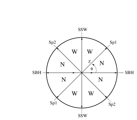
Figure 1: The solution space showing different regions representing naked singularities, wormholes and black holes. Here $\kappa=Z\sin\theta$ and $\lambda=Z\cos\theta$. N–Naked singularities, W–Wormholes, SBH–Schwarzschild black hole, SSW–Spatial Schwarzschild Wormhole, Sp1,2–Special solutions.

To summarize: The $\kappa$–$\lambda$ plane has the following structure (let $\kappa$ run up the vertical axis; and define $\lambda=Z\;\cos\theta$; $\kappa=Z\;\sin\theta$, see figure 1):

• $\theta=0$ (the $+\lambda$ axis): Schwarzschild spacetime.

• $\theta\in(0,\pi/4)$ naked singularity.

• $\theta=\pi/4$ special; see below.

• $\theta\in(\pi/4,3\pi/4)$ traversable wormhole;
  $\theta=\pi/2$ (the $+\kappa$ axis) is the spatial-Schwarzschild wormhole.

• $\theta=3\pi/4$ special; see below.

• $\theta\in(3\pi/4,\pi)$ naked singularity.

• $\theta=\pi$ ($-\lambda$ axis): Schwarzschild spacetime.

• $\theta>\pi$: repeat the previous diagram in the lower half plane.

Let us now look at the two special cases:

• $\theta=\pi/4\quad\Rightarrow\quad\lambda=\kappa$. The geometry is:

  $${\mathrm{d}}s^{2} = -\left\{{2\kappa\over 1+m/2\bar{r}}\right\}^{2}\;{\mathrm{d}}t^{2}$$

  $$+\left(1+{m\over 2\bar{r}}\right)^{4}\left[{\mathrm{d}}\bar{r}^{2}+\bar{r}^{2}\left({\mathrm{d}}\theta^{2}+\sin^{2}\theta\;{\mathrm{d}}\varphi^{2}\right)\right].$$

  The $\bar{r}\rightarrow 0$ region is not flat. (Space is asymptotically flat, but spacetime isn’t since $g_{tt}\to 0$ as $\bar{r}\to 0$.)

• $\theta=3\pi/4\quad\Rightarrow\quad\lambda=-\kappa$. The geometry is:

  $${\mathrm{d}}s^{2} = -\left\{{\kappa m/{\bar{r}}\over 1+m/2\bar{r}}\right\}^{2}\;{\mathrm{d}}t^{2}$$

  $$+\left(1+{m\over 2\bar{r}}\right)^{4}\left[{\mathrm{d}}\bar{r}^{2}+\bar{r}^{2}\left({\mathrm{d}}\theta^{2}+\sin^{2}\theta\;{\mathrm{d}}\varphi^{2}\right)\right].$$

  The $\bar{r}\rightarrow\infty$ region is not flat. (Space is asymptotically flat, but spacetime isn’t since $g_{tt}\to 0$ as $\bar{r}\to\infty$.)

Other interesting features are:

$$g_{tt}(r=\infty)=-(\kappa+\lambda)^{2}$$ (28)

$$g_{tt}(r=0)=-(\kappa-\lambda)^{2}$$ (29)

That is, time runs at different rates in the two asymptotic regions. If we try to reconnect the other side of the wormhole back to our own universe we get a “locally static” wormhole in the sense of Frolov frolov and Novikov novikov .

II.2 Matter fields

We now move on briefly to the generation of the stress energy for the two–parameter asymptotically flat wormhole in $3+1$ dimensions. (The two parameters are $m$ and $\kappa$.) As is well–known, the energy–momentum tensor which acts as a source for the Schwarzschild spacetime with a global monopole can be generated through a triplet of scalar fields $\phi^{a}$ self-interacting via a Higgs potential bv:gm . The Lagrangian for this is:

$$L_{\mathrm{scalar}}=\frac{1}{2}\partial_{\mu}\phi^{a}\;\partial^{\mu}\phi^{a}+\frac{1}{4}\zeta\left(\phi^{a}\phi^{a}-\eta^{2}\right)^{2}$$ (30)

Choosing a monopole-like field configuration $\phi^{a}=\eta\;f(r)\;{x^{a}}/{r}$ we can generate the required stress energy in the region away from the core of the monopole (where $f(r)\equiv 1$ ). Motivated by this model with a triplet of scalar fields, we make an attempt to generate only $\tau$ and $p$ without making any contribution to $\rho$ as required by the Einstein tensor for the line element of the general wormhole discussed in the previous subsection (II.1). To this end, we introduce a Lagrangian with a triplet $\psi^{a}$ given by

$$L_{\mathrm{scalar}}=\frac{1}{2}\partial_{\mu}\psi^{a}\;\partial^{\mu}\psi^{a}+\frac{1}{6}\sigma\left(\psi^{a}{\psi^{a}}\right)^{3}$$ (31)

Assuming a general metric of the form:

$${\mathrm{d}}s^{2}=-B(r)\;{\mathrm{d}}t^{2}+A(r)\;{\mathrm{d}}r^{2}+r^{2}\left({\mathrm{d}}\theta^{2}+\sin^{2}\theta\;{\mathrm{d}}\varphi^{2}\right),$$ (32)

and $\psi^{a}=g(r)\;{x^{a}}/{r}$ we obtain the differential equation for the function $g(r)$:

$$\frac{1}{A}g^{\prime\prime}+\left[\frac{2}{Ar}+\frac{1}{2B}\left(\frac{B}{A}\right)^{\prime}\right]g^{\prime}-\frac{2g}{r^{2}}-\sigma g^{5}=0.$$ (33)

With $g(r)={a}/{\sqrt{r}}$ the above equation results in a constraint on the parameters $a$ and $\sigma$: $\sigma a^{4}=-{9}/{4}$, to leading order in ${1}/{r}$.

The components of the energy momentum tensor are:

$$\rho = T_{00}=\frac{1}{8\pi\;G}\left[\frac{g^{\prime 2}}{2A}+\frac{g^{2}}{r^{2}}+\frac{\sigma}{6}g^{6}\right];$$ (34)

$$\tau = T_{11}=\frac{1}{8\pi\;G}\left[\frac{g^{\prime 2}}{2A}-\frac{g^{2}}{r^{2}}-\frac{\sigma}{6}g^{6}\right];$$ (35)

$$p = T_{22}=T_{33}=\frac{1}{8\pi\;G}\left[-\frac{g^{\prime 2}}{2A}-\frac{\sigma}{6}g^{6}\right].$$ (36)

Assuming that in the asymptotic region $A(r)\to 1$ and $g(r)\to\frac{a}{\sqrt{r}}$ we get:

$$\rho\approx\frac{3a^{2}}{32\pi\;G\;r^{3}};\quad\tau\approx-\frac{a^{2}}{16\pi\;G\;r^{3}};\quad p\approx\frac{a^{2}}{32\pi\;G\;r^{3}}.$$ (37)

From the Einstein tensor for the wormhole, taking $r$ large, we obtain the exact result $\rho=0$ and the approximations

$$\tau\approx-\frac{1}{8\pi\;G}\left[\frac{2m\kappa}{(\lambda+\kappa)r^{3}}\right];\quad p\approx\frac{1}{8\pi\;G}\left[\frac{m\kappa}{(\lambda+\kappa)r^{3}}\right].$$ (38)

Of course, the above stress-energy does not match with the one generated from the scalar field. To match things we add an exotic dust distribution given by:

$$\rho_{d}=-\frac{1}{8\pi\;G}\frac{3a^{2}}{4r^{3}};\qquad\tau_{d}=p_{d}=0.$$ (39)

Notice that this stress energy explicitly violates the energy conditions. The scalar field with a sextic interaction immersed in this dust distribution can give rise to the matter stress energy required for our wormhole, in the large $r$ limit.

For all parameters to exactly match we would require,

$$\frac{a^{2}}{4}=\frac{m\kappa}{\lambda+\kappa}$$ (40)

Thus, in the large $r$ region one can obtain the stresses which generate the metric by using the above scalar field model immersed in a dust distribution of negative energy density.

In closing this section we remind the reader that violations of the energy conditions, though certainly present in wormhole spacetimes, cannot be used (given our current understanding of physics) to automatically rule out wormhole geometries. Indeed over the last few years the catalog of physical situations in which the energy conditions are known to be violated has been growing cosmo99 . There are quite reasonable looking classical systems (non-minimally coupled scalar fields) for which all the energy conditions (including the null energy condition) are violated; and which lead to wormhole geometries barcelo1 ; barcelo2 . In certain branches of physics, most notably braneworld scenarios based on some form of the Randall–Sundrum ansatz, violations of the energy conditions are now so ubiquitous as to be completely mainstream branes . Attitudes regarding the energy conditions are changing, and their violation (even their classical violation) is no longer the anathema it has been in the past.

II.3 Traversability

In the asymptotically flat 3+1 dimensional spacetime discussed in subsection (II.1) we have three parameters: the mass parameter m (or, in dimensionful units ${2GM}/{c^{2}}$) and the two wormhole parameters $\kappa$ (this gets rid of the horizon and ‘makes’ the geometry a wormhole) and $\lambda$. In order to obtain values for each of these or appropriate ratios, we use the well–known traversability constraints discussed by Morris and Thorne mt:ajp88 .

The first constraint as mentioned in MT is related to the acceleration felt by the traveller. Since humans are used to feeling acceleration of order $g$ (earth gravity) we have to ensure this in the trip. The constraint turns out to be:

$$\left|e^{-\Phi}\frac{d(\gamma e^{\Phi})}{dl}\right|\leq\frac{g}{c^{2}}\approx{1\over\hbox{light year}}.$$ (41)

For a traveller moving through the wormhole from one universe to another we must also ensure that the tidal forces which he has to endure should not crush him. If $v$ is the radial velocity of the traveller (whom we assume to be of height $2\;\mathrm{m}$), the tidal forces are related to the projections of the Riemann tensor components along the locally Lorentz frame moving with the traveller. The constraints as outlined by MT are given as:

$$\left|R_{1010}\right|=\left|\left(1-\frac{b}{r}\right)\left(-\Phi^{\prime\prime}+\frac{b^{\prime}r-b}{2r(r-b)}\Phi^{\prime}-{\Phi^{\prime}}^{2}\right)\right|\leq\frac{g}{c^{2}\times 2\;\mathrm{m}}\equiv\frac{1}{(10^{10}\;\mathrm{cm})^{2}}\equiv\frac{1}{(10^{5}\;\mathrm{km})^{2}};$$ (42)

$$\left|R_{2020}\right|=\left|\frac{\gamma^{2}}{2r^{3}}\left[\left(\frac{v}{c}\right)^{2}\left(b^{\prime}-\frac{b}{r}\right)+2(r-b)\Phi^{\prime}\right]\right|\leq\frac{g}{c^{2}\times 2\;\mathrm{m}}\equiv\frac{1}{(10^{10}\;\mathrm{cm})^{2}}\equiv\frac{1}{(10^{5}\;\mathrm{km})^{2}}.$$ (43)

The above Riemann tensor components are obtained by transforming those in the tetrad (frame) basis attached to the Schwarzschild coordinate system to those in a local Lorentz frame moving with a radial velocity $v$. (For details see visser:book , pp 137–143.) For our geometry these constraints turn out to be:

$$\left|\frac{1}{\nu^{\frac{3}{2}}}\;\gamma\;\frac{\lambda}{\kappa\sqrt{\nu}+\lambda\sqrt{\nu-1}}\right|\leq{{2GM}/{c^{2}}\over 1\hbox{ light year}};$$ (44)

$$\left|\frac{1}{\nu^{3}}\;\frac{\lambda\sqrt{\nu-1}}{\kappa\sqrt{\nu}+\lambda\sqrt{\nu-1}}\right|\leq\left(\frac{2GM/c^{2}}{10^{5}\;\mathrm{km}}\right)^{2};$$ (45)

$$\left|\frac{\gamma^{2}}{2}\;\frac{1}{\nu^{3}}\;\left[\frac{\lambda\sqrt{\nu-1}}{\kappa\sqrt{\nu}+\lambda\sqrt{\nu-1}}-\left(\frac{v}{c}\right)^{2}\right]\right|\leq\left(\frac{2GM/c^{2}}{10^{5}\;\mathrm{km}}\right)^{2}.$$ (46)

where $\nu\equiv r/(2m)$. In particular $\nu\geq 1$ (we are now using Schwarzschild coordinates and $\nu=1$ is the throat of the wormhole).

Picking values of $\nu$ and $v$ we can calculate the acceptable range of values for the parameters $m$, $\kappa$, and $\lambda$ which appear in the line element. This would determine for us the actual geometry of a macroscopic traversable wormhole without any unknown, to–be–determined constants. As an example we choose $\nu=1$ (at the throat of the wormhole). Assuming $r=2m\equiv 10^{5}\;\mathrm{km}$ we find that $\kappa/\lambda\geq 10^{8}\;\gamma$ and $\gamma^{2}\beta^{2}<2$, implying $\beta<\sqrt{2/3}$. One can obtain similar bounds by assuming other values for the throat radius.

III Conclusions

Let us now summarize the results obtained. We set out with the goal of obtaining wormholes through a certain geometric prescription. To this end we proposed $\rho=\rho_{t}=0$ as the characterizing equation on the spacetime (which also implies $R=0$, i.e., $\rho=\rho_{t}$, and, equivalently, traceless stress energy). The shape function $b(r)$ is determined by the condition $\rho=0$. Solving the ensuing differential equation for the $R=0$ condition we obtain the red-shift function $\phi(r)$. The resulting line element represents a two-parameter family of geometries which contains Lorentzian wormholes, naked singularities, and the Schwarzschild black hole. Using isotropic coordinates we subsequently displayed the full structure of the solution space of the relevant equations, discussing the domains in $\kappa$–$\lambda$ parameter space for which these geometries arise.

The matter stress energy for the $R=0$ solutions is obtained thereafter through a model with a triplet scalar field in a sextic potential, superimposed upon a dust distribution of negative energy density. Finally the traversability constraints are written down and analysed.

Our aim in this paper has been to provide a prescription for obtaining wormholes. We have proposed one such prescription which is characterized by the equation $\rho=\rho_{t}=0$. This would imply $R=0$. One can also generalize this further and look into the solution space of similar characterizing equations/relations which yield wormholes and other solutions. Additionally, instead of $R=0$ one might want to obtain constant curvature wormholes which belong to the class of spaces known as Einstein spaces. Future work along these lines, will, hopefully shed light on these features in greater detail.

As a punchline, we mention that the equation we propose implies the curious fact that the Schwarzschild black hole is not as unique as it is believed to be — it is intimately related to a host of traversable wormholes; solutions to the differential equations $R=0$ and $\rho=0$. We normally discard them on account of violation of the energy conditions. Alternatively, taking a more liberal viewpoint, we might retain them as tentative models awaiting confirmation through future observations. This is particularly pertinent in view of the recent developments in braneworld physics, where there is a marked change in attitude towards the energy conditions. Attitudes now tend to be more accommodating and liberal.

References

- (1) M. S. Morris, K. S. Thorne and U. Yurtsever, “Wormholes, Time Machines, And The Weak Energy Condition”, Phys. Rev. Lett. 61 (1988) 1446.
- (2) M. S. Morris and K. S. Thorne, “Wormholes In Space-Time And Their Use For Interstellar Travel: A Tool For Teaching General Relativity”, Am. J. Phys. 56 (1988) 395.
- (3) H. Epstein, E. Glaser, and A. Yaffe, Nuovo Cimento 36, 1016 (1965)
- (4) M. Visser, Lorentzian wormholes: from Einstein to Hawking, AIP Press (1995).
- (5) M. Visser and D. Hochberg, “Geometric wormhole throats”, gr-qc/9710001.
-
(6)
D. Hochberg,
“Lorentzian Wormholes In Higher Order Gravity Theories”,
Phys. Lett. B 251 (1990) 349.
B. Bhawal and S. Kar, “Lorentzian wormholes in Einstein-Gauss-Bonnet theory”, Phys. Rev. D 46 (1992) 2464. -
(7)
S. Kar,
“Evolving wormholes and the weak energy condition”,
Phys. Rev. D 49 (1994) 862.
S. Kar and D. Sahdev, “Evolving Lorentzian wormholes”, Phys. Rev. D 53 (1996) 722 [gr-qc/9506094]. -
(8)
D. Hochberg and M. Visser,
“The null energy condition in dynamic wormholes”,
Phys. Rev. Lett. 81, 746 (1998)
[gr-qc/9802048].
D. Hochberg and M. Visser, “Dynamic wormholes, anti-trapped surfaces, and energy conditions”, Phys. Rev. D 58 (1998) 044021 [gr-qc/9802046]. - (9) D. Hochberg and M. Visser, “General dynamic wormholes and violation of the null energy condition”, gr-qc/9901020.
-
(10)
J. G. Cramer, R. L. Forward, M. S. Morris, M. Visser, G. Benford and
G. A. Landis,
“Natural wormholes as gravitational lenses”,
Phys. Rev. D 51 (1995) 3117
[astro-ph/9409051].
L. A. Anchordoqui, G. E. Romero, D. F. Torres and I. Andruchow, “In search for natural wormholes”, Mod. Phys. Lett. A 14 (1999) 791 [astro-ph/9904399].
M. Safonova, D. F. Torres and G. E. Romero, “Microlensing by natural wormholes: Theory and simulations”, [gr-qc/0105070].
M. Safonova, D. F. Torres and G. E. Romero, “Macrolensing signatures of large-scale violations of the energy conditions”, Mod. Phys. Lett. A 16 (2001) 153 [astro-ph/0104075].
E. Eiroa, G. E. Romero and D. F. Torres, “Chromaticity effects in microlensing by wormholes”, Mod. Phys. Lett. A 16 (2001) 973 [gr-qc/0104076]. - (11) N. Dadhich, “Spherically symmetric empty space and its dual in general relativity”, Curr. Sci. 78 (2000) 1118 [gr-qc/0003018].
-
(12)
N. Dadhich,
“A duality relation: Global monopole and texture”,
gr-qc/9712021.
N. Dadhich, “On electrogravity duality”, Mod. Phys. Lett. A 14 (1999) 337 [gr-qc/9805068]. - (13) S. Kar and D. Sahdev, “Restricted class of traversable wormholes with traceless matter”, Phys. Rev. D 52 (1995) 2030.
- (14) V. P. Frolov, “Vacuum polarization in a locally static multiply connected space-time and a time machine problem”, Phys. Rev. D 43 (1991) 3878.
- (15) V. P. Frolov and I. D. Novikov, “Physical Effects In Wormholes And Time Machine”, Phys. Rev. D 42 (1990) 1057.
- (16) M. Barriola and A. Vilenkin, “Gravitational Field Of A Global Monopole”, Phys. Rev. Lett. 63 (1989) 341.
- (17) M. Visser and C. Barcelo, “Energy conditions and their cosmological implications”, gr-qc/0001099.
- (18) C. Barcelo and M. Visser, “Traversable wormholes from massless conformally coupled scalar fields”, Phys. Lett. B 466 (1999) 127 [gr-qc/9908029].
- (19) C. Barcelo and M. Visser, “Scalar fields, energy conditions, and traversable wormholes”, Class. Quant. Grav. 17 (2000) 3843 [gr-qc/0003025].
- (20) C. Barcelo and M. Visser, “Brane surgery: Energy conditions, traversable wormholes, and voids”, Nucl. Phys. B 584 (2000) 415 [hep-th/0004022].