Constraints on spatial distributions of negative energy

Abstract

This paper initiates a program which seeks to study the allowed spatial distributions of negative energy density in quantum field theory. Here we deal with free fields in Minkowski spacetime. Known restrictions on time integrals of the energy density along geodesics, the averaged weak energy condition and quantum inequalities are reviewed. These restrictions are then used to discuss some possible constraints on the allowable spatial distributions of negative energy. We show how some geometric configurations can either be ruled out or else constrained. We also construct some explicit examples of allowed distributions. Several issues related to the allowable spatial distributions are also discussed. These include spacetime averaged quantum inequalities in two-dimensional spacetime, the failure of generalizations of the averaged weak energy condition to piecewise geodesics, and the issue of when the local energy density is negative in the frame of all observers.

I Introduction

The energy density of all observed forms of classical matter is non-negative. However, quantum field theory has the remarkable property that the local energy density can be negative. This violates the weak energy condition (WEC) which postulates that the local energy density is non-negative for all observers. Its formal statement is that a stress tensor $T_{\mu\nu}$ satisfies the WEC provided that

$$T_{\mu\nu}\,u^{\mu}\,u^{\nu}\,\geq 0\,,$$ (1)

for all timelike vectors $u^{\mu}$. Negative energy densities raise the possibility of a variety of exotic phenomena, including violations of the second law of thermodynamics Ford (1978); Davies (1982), traversable wormholes Morris and Thorne (1988); Morris et al. (1988) and “faster-than-light” travel Alcubierre (1994); Olum (1998); Gao and Wald (2000), creation of naked singularities Ford and Roman (1990, 1992), and avoidance of singularities in gravitational collapse. However, in the case of inflationary cosmology it has recently been found that violations of the WEC do not allow one to avoid initial singularities Borde et al. (2001).

I.1 Brief review of averaged weak energy conditions and quantum inequalities

The interest attached to the effects of negative energy has stimulated the study of constraints on the magnitude and extent of WEC violations. Although the energy density at a point can be arbitrarily negative, there are several integral constraints which we will briefly review for the case of flat spacetime. One constraint is that the integral of the energy density over all space, the Hamiltonian, is bounded below. Other constraints involve integrals over the world line of an observer, a construction first introduced by Tipler Tipler (1978). One such constraint is the averaged weak energy condition (AWEC), which states that the integral of the energy density seen by a geodesic observer is non-negative:

$$\int_{-\infty}^{\infty}T_{\mu\nu}\,u^{\mu}\,u^{\nu}\,d\tau\geq 0\,.$$ (2)

Here $u^{\mu}$ and $\tau$ are the observer’s four-velocity and proper time, respectively. This condition has been proven to hold for a variety of free quantum field theories in boundary-free Minkowski spacetime. It does not always hold inside of a cavity in flat spacetime because the Casimir energy density can be negative. However, even in this case, observers at rest with respect to the cavity walls will see a modified version of Eq. (2) satisfied. This is the “difference AWEC” in which $T_{\mu\nu}$ is replaced by the difference between the expectation value of the stress tensor in an arbitrary quantum state and that in the vacuum state Ford and Roman (1995); Mitch98 . The physical content of this statement is that although the local energy density can be made more negative than in the vacuum, the time-integrated energy density cannot. A related averaged energy condition is the averaged null energy condition (ANEC), in which the integration is along a null geodesic. It also holds in boundary-free Minkowski spacetime Wald and Yurtsever (1991). The extent to which the AWEC and ANEC hold for quantum field theories in curved spacetime is less clear Yurtsever (1990); Visser (1995); Flanagan and Wald (1996).

Although the AWEC imposes a significant constraint on negative energy, even stronger constraints are available in the form of “quantum inequalities”, (QIs) Ford (1978, 1991); Ford and Roman (1995, 1997); Flanagan (1997); Pfenning and Ford (1997); Fewster and Eveson (1998). These are lower bounds on time integrals of the energy density multiplied by a sampling function, $g(t)$:

$$\int_{-\infty}^{\infty}T_{\mu\nu}\,u^{\mu}\,u^{\nu}\,g(t)\,dt\geq{\hat{\rho}}_{min}\,.$$ (3)

The lower bound, ${\hat{\rho}}_{min}$, depends upon the sampling function and upon the spacetime. For the massless scalar field in two-dimensional Minkowski spacetime, Flanagan Flanagan (1997) has found the optimal bound:

$${\hat{\rho}}_{min}=-\frac{1}{24\,\pi}\,\int_{-\infty}^{\infty}\,\frac{{g^{\prime}(t)}^{2}}{g(t)}\,dt\,.$$ (4)

For the massless scalar field in four-dimensional Minkowski spacetime, Fewster and Eveson Fewster and Eveson (1998) have given a similar (but not necessarily optimal) bound:

$${\hat{\rho}}_{min}=-\frac{1}{16\,{\pi}^{2}}\,\int_{-\infty}^{\infty}\,{\bigl{(}{g^{1/2}}^{\prime\prime}(t)\bigr{)}}^{2}\,.$$ (5)

If the sampling function has a characteristic width $t_{0}$, then the lower bounds are of the form

$${\hat{\rho}}_{min}=\frac{C}{t_{0}^{D}}\,,$$ (6)

where $D$ is the dimensionality of spacetime. The AWEC can be derived from the QIs as the limit in which $t_{0}\rightarrow\infty$. The essential physical content of the QIs is that the larger a pulse of negative $(-)$ energy is, the closer in time it must be to a compensating pulse of positive $(+)$ energy. Consider for example $\delta$-function pulses of $(+)$ and $(-)$ energy where the energy density in an observer’s frame is given by

$$\rho(t)=B\,[-\delta(t)+(1+\epsilon)\,\delta(t-T)]\,.$$ (7)

Here $T$ is the temporal separation of the pulses and $B$ is either the magnitude $|\Delta E|$ of the $(-)$ pulse in two dimensions, or the magnitude of its energy per unit area $|\Delta E|/A$ in four dimensions. It may be shown from the QIs Ford and Roman (1999) that

$$T\leq\frac{K_{2}}{|\Delta E|}\,,$$ (8)

in two dimensions and

$$T\leq K_{4}\,{\biggl{(}\frac{A}{|\Delta E|}\biggr{)}}^{1/3}\,,$$ (9)

in four dimensions, where the dimensionless constants $K_{2}$ and $K_{4}$ are typically less than unity. Thus as the strength $|\Delta E|$ of the $(-)$ pulse increases, its separation in time from the compensating $(+)$ pulse must decrease as an inverse power of $|\Delta E|$.

In Ref. Ford and Roman (1999) it is further shown that the QIs imply the phenomenon of quantum interest. As the temporal separation of the $(-)$ and $(+)$ pulses increases, within the limits set by Eqs. (8) and (9), the degree of overcompensation must increase. Thus the parameter $\epsilon$ must be a monotonically increasing function of $T$. A discussion of quantum interest for more general pulses was given by Pretorius Pretorius (2000) and by Fewster and Teo Fewster and Teo (2000).

I.2 The program

The purpose of this paper is to initiate an exploration of the limits on the spatial distribution of $(-)$ energy. The worldline QIs summarized in the previous subsection provide one tool for this investigation. Clearly, for massless fields, the temporal separation of a pair of pulses as seen by an inertial observer is also a measure of their spatial separation. However, a more detailed picture is desirable. Several approaches can be pursued in the search for a description of the allowed spatial $(-)$ energy distributions. One is to seek generalizations of the QIs which involve averaging over space as well as time. Another approach is to use the AWEC and QIs to place constraints upon the allowed spacetime distributions. The approach seeks to extract as much information as possible from the requirement that the AWEC and QIs be satisfied along all timelike geodesics. A third approach is to examine the nature of distributions which are definitely allowed and can be explicitly constructed. All three approaches will be illustrated in this paper.

I.3 Outline of this paper

This paper will deal entirely with $(-)$ energy distributions in flat spacetime. In Sec. II.1, we review and discuss two results which suggest that arbitrarily large amounts of $(-)$ energy can be concentrated in a given region of space. As a counterpoint, we show in Sec. II.2 that in two spacetime dimensions, there are both spatial and spacetime averaged versions of the quantum inequalities. We next turn in Sec. III to a discussion of several model $(-)$ energy distributions which the AWEC and QIs either forbid (Sec. III.1), or else quantitatively constrain (Sec. III.2). Section IV is devoted to the explicit construction of some informative examples of allowed distributions. In particular, the energy distribution of a massive scalar field in a single wavepacket mode squeezed state is used to illustrate the convoluted way in which $(-)$ and $(+)$ energy can be entwined. As part of this discussion, it is useful to distinguish between WEC violations in which the local energy density is negative for all observers (“strong” violations), and those in which its sign depends upon the observer (“weak” violations). The technical details of this distinction are elaborated in the Appendix. Section V explores the limits of the AWEC, and shows that it would not hold if one were to integrate along a piecewise geodesic path. Similarly, the “difference AWEC” need not hold for the quantum field stress tensor in a cavity in the case of an observer who passes through the cavity. This section also uses the cavity example to illustrate strong and weak WEC violations. Finally, our results are summarized and discussed in Sec. VI. Units in which $\hbar=c=1$ and a spacelike metric convention are used in this paper.

II Difficulties with spatial bounds?

II.1 Two Disturbing Results

There are two disturbing results which might be construed as casting doubt upon the existence of constraints on the spatial distribution of negative energy. The first is an unpublished result of Garfinkle Garfinkle (1990), who showed that the total energy contained within an imaginary box in Minkowski spacetime is unbounded below. Let us first give a more precise statement of this result. Consider a quantum field $\varphi$ in boundary-free Minkowski spacetime. By boundary-free, we mean that there are no physical boundaries upon which $\varphi$ must satisfy boundary conditions. Let $\rho=:T_{tt}:$ be the normal-ordered energy density operator for $\varphi$ on a $t=$ constant hypersurface. Now consider a volume $V$, e.g., the interior of an arbitrary rectangular box, and let

$$E=\int_{V}\langle\psi|\rho|\psi\rangle\,d^{3}x$$ (10)

be the energy inside this box in quantum state $|\psi\rangle$. This box is “imaginary” in the sense that there are no physical boundaries at the walls of the box. The Garfinkle result is that $E$ is unbounded below. That is, there exist states $|\psi\rangle$ for which $E$ is arbitrarily negative. Note that this would not happen if the box were a physical box on whose walls $\varphi$ must satisfy Dirichlet or Neumann boundary conditions. In this case, $E$ is the Hamiltonian for $\varphi$ within this cavity, and is bounded below by the Casimir energy of the cavity.

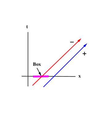
Figure 1: The Garfinkle box is illustrated. A $\delta$-function pulse of $(+)$ energy has already passed through the box before time $t=0$. At time $t=0$, a $\delta$-function pulse of $(-)$ energy is inside the box. The magnitude of this $(-)$ pulse is inversely related to the distance to the $(+)$ pulse at a fixed time. However, we can always arrange for the $(+)$ pulse to be just outside the box, and for the $(-)$ pulse to be just inside. Thus there can be an arbitrary amount of $(-)$ energy inside the box at $t=0$.

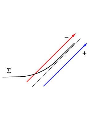
Figure 2: Here $\Sigma$ is a spacelike hypersurface which is asymptotic to a null surface, the dashed line. This allows $\Sigma$ to catch a $\delta$-function pulse of $(-)$ energy, while also avoiding the compensating $\delta$-function pulse of $(+)$ energy. In this way, the integrated energy over $\Sigma$ may be made arbitrarily negative.

A second disturbing result was given by Helfer Helfer (1996), who showed that the integral of the energy density over a spacelike hypersurface can be unbounded below. Although this result applies to curved, as well as flat spacetime, let us focus on the case of Minkowski spacetime. Let $\xi^{\mu}$ be a timelike vector field on Minkowski spacetime, and let $\Sigma$ be a spacelike hypersurface to which $\xi^{\mu}$ is orthogonal. Further let

$$\hat{H}(\xi,\Sigma)=\int\langle\psi|T^{\mu\nu}\,\xi_{\mu}\,\xi_{\nu}|\psi\rangle\,f\,dv\,.$$ (11)

Here $dv$ is the volume element in $\Sigma$, and $f$ is a test function with compact support. The quantity $\hat{H}(\xi,\Sigma)$ is an energy operator (generalized Hamiltonian) obtained by integrating the energy density in state $|\psi\rangle$ (times the test function $f$) over $\Sigma$. Helfer has shown that in general, $\hat{H}(\xi,\Sigma)$ is unbounded below. Note that in the limit that $f\rightarrow 1$ everywhere and $\xi^{\mu}$ is the timelike Killing vector, $\hat{H}(\xi,\Sigma)$ becomes the usual Hamiltonian, which has the lower bound of zero, attained in the Minkowski vacuum state. Note also that the Helfer result includes the Garfinkle result as the special case in which $\Sigma$ is a constant $t$ (Minkowski time) surface and $f$ approaches a step function which is $1$ inside the box and $0$ outside of it.

Both of these results might lead one to conclude that there can be no bounds on the spatial distribution of negative energy which would be analogous to the temporal bounds given by the quantum inequalities. Thus it is desirable to understand the physical basis of these results in more detail.

Consider first the Garfinkle box. We can understand the unboundedness of the total energy $E$ in this box as arising from two factors: (1) The energy is measured at a precise instant in time, and (2) the walls of the box are sharply defined. This allows an arbitrary amount of negative energy to have entered the box by time $t$, while at this time excluding an even larger amount of positive energy which may be just outside of the box at time $t$. This situation is illustrated in Fig. 1.

The unboundedness of Helfer’s $\hat{H}$ is harder to understand, although in particular cases one can give intuitive explanations similar to that in the Garfinkle box case. Let the hypersurface $\Sigma$ be asymptotically null, as illustrated in Fig. 2. In this case, it is possible for the integral of the energy density over $\Sigma$ to include the contribution of an arbitrarily large negative energy pulse, but to omit that of an even larger positive pulse which preceded the negative pulse. Once we include the effects of the test function $f$, it is not necessary that $\Sigma$ be asymptotically null; it can level out and approach a constant $t$ surface outside of the domain of support of $f$.

These considerations might suggest that the Garfinkle and Helfer results arise by methods of spatial averaging which manage to capture large amounts of $(-)$ energy while ignoring larger amounts of $(+)$ energy which are really very close by. However, the general result of Helfer is not so easily explained. Even if $\Sigma$ is a constant $t$ surface, $\hat{H}$ need not be bounded below in general in four-dimensional spacetime. In this case, we are dealing with the generalization of the Garfinkle result where the walls of the box cease to be sharply defined. This seems to suggest that spatial averaging without time averaging may not be sufficient to yield quantities which are bounded below.

II.2 Spacetime averaged quantum inequalities in two dimensions

We now turn to the question of whether one can derive generalizations of the quantum inequalities which involve averaging over both space and time. In two-dimensional spacetime, this can indeed be done. This was first done by one of us Roman (1997) using a method analogous to those used in Ref. Ford (1991) to first prove worldline quantum inequalities. Flanagan Flanagan (1997) later noted that his method may also be used to generate two-dimensional spacetime averaged quantum inequalities. Let $\sigma(u,v)$ be a spacetime sampling function, where $u=t-x$ and $v=t+x$ are null coordinates. We will assume that this function can be expressed as a product of sampling functions in space and time separately in some frame of reference:

$$\sigma(u,v)=g_{T}(t)\,g_{S}(x)\,.$$ (12)

The sampled energy density is

$$\hat{\rho} = \int T_{tt}\,g_{T}(t)\,g_{S}(x)\,dt\,dx$$ (13)

$$= \frac{1}{2}\int[T_{uu}(u)+T_{vv}(v)]\,\sigma(u,v)\,du\,dv\,.$$

Let

$$g_{1}(u)=\frac{1}{2}\int\sigma(u,v)\,dv$$ (14)

and

$$g_{2}(v)=\frac{1}{2}\int\sigma(u,v)\,du\,.$$ (15)

The various sampling functions are normalized so that

$$\int\,g_{T}(t)\,g_{S}(x)\,dt\,dx = \frac{1}{2}\int\sigma(u,v)\,du\,dv$$

$$=\int g_{1}(u)\,du\, = \int g_{2}(v)\,dv=1\,.$$ (16)

We can now write the spacetime averaged quantum inequality as

$$\hat{\rho} = \int T_{uu}(u)\,g_{1}(u)\,du+\int T_{vv}(v)\,g_{2}(v)\,dv$$ (17)

$$\geq -\frac{1}{48\,\pi}\left[\int_{-\infty}^{\infty}du\,\frac{(g_{1}^{\prime})^{2}}{g_{1}}+\int_{-\infty}^{\infty}dv\,\frac{(g_{2}^{\prime})^{2}}{g_{2}}\right]\,.$$

In the last step, we used Flanagan’s result, Eq. (4).

Let us explicitly evaluate the bound for some particular sampling functions. First consider Lorentzian functions in both space and time, with widths $x_{0}>0$ and $t_{0}>0$, respectively:

$$g_{S}(x)=\frac{x_{0}}{\pi(x^{2}+x_{0}^{2})}\,,\qquad g_{T}(t)=\frac{t_{0}}{\pi(t^{2}+t_{0}^{2})}\,.$$ (18)

These choices lead to

$$g_{1}(u)=\frac{x_{0}+t_{0}}{\pi[(x_{0}+t_{0})^{2}+u^{2}]}\,,$$ (19)

and $g_{2}(v)=g_{1}(v)$. The bound on the spacetime averaged energy density now becomes

$$\hat{\rho}\geq-\frac{1}{48\,\pi\,(x_{0}+t_{0})^{2}}\,.$$ (20)

A second possible choice of sampling function is a Gaussian in both space and time:

$$g_{S}(x)=\frac{1}{\sqrt{\pi}x_{0}}\,{\rm e}^{-x^{2}/x_{0}^{2}}\,,\qquad g_{T}(t)=\frac{1}{\sqrt{\pi}t_{0}}\,{\rm e}^{-t^{2}/t_{0}^{2}}\,.$$ (21)

In this case, we find

$$g_{1}(u)=\frac{1}{\sqrt{\pi(x_{0}^{2}+t_{0}^{2})}}\,{\rm e}^{-u^{2}/(x_{0}^{2}+t_{0}^{2})}\,,$$ (22)

and the bound becomes

$$\hat{\rho}\geq-\frac{1}{12\,\pi\,(x_{0}^{2}+t_{0}^{2})}\,.$$ (23)

These spacetime averaged quantum inequalities reduce to the usual QIs along worldlines in the limit that $x_{0}=0$. Note that in two dimensions one also has a nontrivial bound from spatial averaging alone when $t_{0}=0$. The extent to which the type of results found here in two dimensions can be generalized to four dimensions is unclear. It seems that there one may need the temporal averaging to get a bound.

III Forbidden and constrained distributions

We can rule out several spatial distributions of $(+)$ and $(-)$ energy by applying the AWEC and the QIs to their possible evolutions. In all of the examples given below we assume that the violations of the WEC are strong, i.e., if the energy density is negative in one frame then it is negative in all frames. (See the Appendix for further details.) This assumption is necessary for the following discussion. In most of the cases we will be specifically considering null fluids, i.e.,

$$T^{\mu\nu}=\rho\,k^{\mu}k^{\nu}\,.$$ (24)

For such stress tensors the violations of the WEC are strong, as can be easily shown. We will explicitly point out the situations in which we do not assume this form for the stress tensor.

III.1 Forbidden distributions

III.1.1 Separated regions of $(+)$ and $(-)$ energy, with the $(+)$ energy moving rigidly

Consider an initial state that consists of a compact region, $\cal N$, of $(-)$ energy and a distinct compact region, $\cal P$, of $(+)$ energy. The compactness of the initial $(+)$ energy distribution (i.e., its finite spatial extent) is crucial to the arguments that we present. We assume that $\cal P$ does not embrace $\cal N$ in the sense that both regions can be contained in non-intersecting rectangular boxes.

We consider situations in which the $(+)$ energy moves “rigidly” in that the null flow vector $k^{\mu}$ in the energy-momentum tensor, Eq. (24), is constant in Cartesian coordinates. More general evolutions are discussed in Sec. III.2. The $(-)$ energy may evolve in any way that it likes.

Let $O$ be any point in $\cal N$ and choose Cartesian coordinates with $O$ at the origin. The time axis will be the straight line that passes through $O$ in the time direction ($x=y=z=0$). Consider the world tube that represents the evolution of $\cal P$, extended as far as possible in both future and past directions. If this world tube never crosses the time axis, an observer sitting on the axis throughout will never encounter the $(+)$ energy and his worldline will violate the AWEC.

Figure 3: The world tube of the $(+)$ energy region cannot “cap the future light cone” of a point, $O$, in the $(-)$ energy region.

Next, consider the case where the world tube crosses the time axis in the future direction. (The case when it crosses it in the past direction is covered by the time-reverse of the argument presented below.) This means that the positive energy flows across the future of the region where there was negative energy, as shown in Fig. 3. Since the motion of the positive energy is rigid, its world tube does not expand in either time direction. Thus, although it will cross the future light cone of a point in the negative energy region, it cannot entirely “cap” that light cone. Suitably chosen timelike geodesics that go through the negative energy can avoid intersecting any positive energy at all. We prove this precisely below.

In the case where the crossing takes place in the future, no timelike geodesic through $O$ can intersect the world tube of $\cal P$ in the past, since in the past direction the world tube is running away from the origin at the speed of light. We show that there is at least one geodesic that avoids intersecting the world tube of $\cal P$ in the future direction as well. We choose our Cartesian coordinates so that the positive $y$ direction is the direction of motion of the $(+)$ energy and we set things up at $t=0$ as follows: Let $P=(0,x_{0},y_{0},z_{0})$ be a point in $\cal P$ with the property that no point in $\cal P$ has a larger $x$-coordinate. The compactness of $\cal P$ guarantees that there will be such a point. This point will lie on an “edge” of $\cal P$ in the $x$ direction. The choice of $x$ is arbitrary. We could just as well make the argument we are about to make below by choosing a point on the edge in the $z$ direction. By the assumptions that the $(+)$ energy does not embrace the $(-)$ energy and that the $(+)$ energy is moving towards the origin in the positive $y$ direction, we have $y_{0}<0$.

Since the world tube of $\cal P$ moves rigidly in the $y$ direction, we note that no point on this world tube can have an $x$ coordinate larger than $x_{0}$. Our strategy is to show that there are timelike geodesics that pass through the origin and escape to a point with $x$ coordinate equal to $x_{0}$ without intersecting the $(+)$ energy (i.e., the world tube of $\cal P$). Since the $x$ coordinate on such a geodesic must continue to increase, it can never intersect the world tube of $\cal P$ if it has not already done so by this stage.

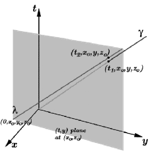
Figure 4: An illustration of the argument of Sec. III.1.1. The timelike geodesic $\gamma$ from the origin gets to point $(x_{0},y,z_{0})$ on the $(t,y)$ plane at $(x_{0},y_{0})$, the shaded region, before the null geodesic $\lambda$ gets to the same spatial point.

Let $\lambda$ be the null geodesic in the world tube of $\cal P$ that passes through $P$ and points in the direction of the flow vector $k^{\mu}$. It will obey the equations $t=y-y_{0},x=x_{0},z=z_{0}$ and so lies in the $t$-$y$ plane located at $(x_{0},z_{0})$, as depicted in Fig. 4. Now consider an arbitrary timelike geodesic, $\gamma$, through $O$. It will obey $t^{2}=\alpha^{2}(x^{2}+y^{2}+z^{2})$, where $\alpha>1$. If such a $\gamma$ can get to some spatial point $(x_{0},y,z_{0})$, with $y>0$, in the $t$-$y$ plane of interest before $\lambda$ gets there, then, as we have seen, $\gamma$ can avoid intersecting any positive energy. We show that it is possible for $\gamma$ to do this. Suppose that $\gamma$ gets to $(x_{0},y,z_{0})$ at time $t_{1}$ and $\lambda$ gets there at time $t_{2}$. The condition $t_{2}>t_{1}$ for $\lambda$ to get to this spatial point after $\gamma$ can be expressed as $(y-y_{0})^{2}>\alpha^{2}(x_{0}^{2}+y^{2}+z_{0}^{2})$, or

$$\alpha^{2}x_{0}^{2}+\alpha^{2}z_{0}^{2}<-y^{2}(\alpha^{2}-1)-2yy_{0}+y_{0}^{2}.$$ (25)

Since $y_{0}<0$ and $y>0$, the only negative term on the right is the first one. Choosing $\alpha^{2}=1+(y_{0}^{2}/2y^{2})$, we see that (i) the first and third terms on the right combine to give a positive value, and (ii) for large $y$, we have $\alpha^{2}$ close to $1$. By choosing $y$ sufficiently large, then, we can make the right hand side as big as we want while keeping the left hand side close to $x_{0}^{2}+z_{0}^{2}$. Therefore, irrespective of the values of $x_{0}$ and $z_{0}$, we can find a value of $y$ (with $\alpha^{2}$ chosen as above) so as to satisfy inequality (25). Thus, we have shown that it is possible to find a timelike geodesic that outruns the positive energy to an edge of the spatial region that the positive energy can cover. This geodesic only passes through negative energy – a forbidden scenario.

The argument covers any finite initial distribution of a $(+)$ energy null fluid, no matter how large, and any initial distribution of $(-)$ energy, no matter how small, as long as the $(+)$ energy moves rigidly in one direction. The $(+)$ energy cannot fully “cap the future light cone” of a $(-)$ energy point, as illustrated in Fig. 3. Some timelike geodesics are guaranteed to escape without intersecting any $(+)$ energy. If we want the AWEC to hold along every timelike geodesic, then even if there is a single point at which negative energy exists we need an infinitely large distribution of compensating positive energy.

Our argument applies to any shape of $(+)$ and $(-)$ energy distribution. In particular, it covers $(+)$ and $(-)$ energy “pancakes”. These are distributions that are small in one spatial direction compared to the other two.

III.2 Constrained distributions

III.2.1 Separated regions of $(+)$ and $(-)$ energy, with the $(+)$ energy moving arbitrarily

If the $(+)$ energy does not move rigidly, the configuration discussed in Sec. III.1.1 cannot be ruled out, in general, on the grounds that there will always be a timelike geodesic that intersects the $(-)$ energy but not the $(+)$. If the $(+)$ energy expands outward, for instance, no timelike geodesic through $(-)$ can outrun the world tube of the $(+)$ energy. Even in this case, however, by choosing a timelike geodesic that is close enough to a null one we can put off the encounter with the positive energy as late as we like. If the distribution of $(+)$ energy is expanding, its density may then be dilute enough so as to be insufficient to enforce the AWEC. This will happen in the case when the $(+)$ energy expands outward uniformly, so that its density $\rho$ goes down everywhere as $1/t^{3}$.

III.2.2 Pancakes

Let us first consider a box-like region of $(-)$ energy which moves in the $x$-direction at the speed of light. If the box has a constant energy density of magnitude $|\rho|$, how large can the box be? Presumably there is some $(+)$ energy nearby, as required by the AWEC and the QIs. However, if we use a compactly-supported sampling function which cuts off rapidly near the edge of the $(-)$ energy region, we can get a bound on the size of the $(-)$ energy region alone.

Assume the density, $-|\rho|$, is that measured in the frame of reference of an observer $O$ who is at rest on the $x$-axis. We further assume that the stress tensor has the null fluid form given by Eq. (24), with $\rho=-|\rho|$. Take $k^{\mu}=(1,1,0,0)$. The observer’s four velocity is $u^{\mu}=(1,0,0,0)$. Therefore $T_{\mu\nu}u^{\mu}u^{\nu}=-|\rho|$. The QI applied in $O$’s frame is

$$-\int_{-\infty}^{\infty}\,g(t)|\rho|\,dt\geq-\frac{C}{{t_{0}}^{4}}\,.$$ (26)

Here the Minkowski time $t$ is the proper time along $O$’s worldline and $t_{0}$ is the sampling time, which we set equal to the time $O$ spends in the $(-)$ energy region. Let the $x$-dimension of the box, as measured by $O$, be $L_{x}$. Since the box moves past $O$ along the $x$-axis at the speed of light, the time for the box to pass $O$ is $t_{0}=L_{x}$. Using Eq. (26), and the fact that $\rho$ is a constant and the sampling function is compactly-supported with unit norm, we obtain the bound

$$L_{x}\leq{\left(\frac{C}{|\rho|}\right)}^{1/4}\,.$$ (27)

Can we get a stronger bound using observers boosted in the $x$-direction? First consider an observer $O^{\prime}$ who is boosted along the $x$-axis. His four velocity is $u^{\mu}=(\gamma,v\gamma,0,0)$, where $\gamma=1/\sqrt{1-v^{2}}$, and $T_{\mu\nu}u^{\mu}u^{\nu}=-|\rho|\,(1-v)/(1+v)$. The QI applied in $O^{\prime}$’s frame is

$$-\int_{-\infty}^{\infty}\,g(\tau)|\rho|\,\left(\frac{1-v}{1+v}\right)\,d\tau\geq-\frac{C}{{\tau_{0}}^{4}}\,.$$ (28)

Here $\tau$ is $O^{\prime}$’s proper time coordinate and the sampling time $\tau_{0}$ is the time $O^{\prime}$ spends in the $(-)$ energy. The time $\tau_{0}$ for the box to pass $O^{\prime}$ is $\tau_{0}=L_{x}/\gamma$. Using Eq. (28), we get the following bound on $L_{x}$:

$$L_{x}\leq{\left(\frac{C}{|\rho|}\right)}^{1/4}\left[\frac{1}{{(1-v)}^{3/4}{(1+v)}^{1/4}}\right]\,.$$ (29)

The righthand side has a minimum at $v=-1/2$. The resulting bound is

$$L_{x}\leq 0.877\,{\left(\frac{C}{|\rho|}\right)}^{1/4}\,,$$ (30)

which is slightly stronger than Eq. (27).

Can we constrain the other dimensions of the box by examining observers who are boosted in directions transverse to the box’s direction of motion? It would appear not. Consider an observer shot through the box along the $y$-axis. The maximum time the observer can spend in the $(-)$ energy is ultimately determined by how long the box takes to pass him, which in turn depends only on its length along its direction of motion. The latter is bounded by Eq. (30). Note that the length of the $y$-dimension of the box could be as large as we like. How far the observer can travel in this direction, while still remaining in the $(-)$ energy, depends on how long it takes the back wall of the box to hit him. Hence it appears that we can make the transverse dimensions of the box as large as we like.

The previous discussion leads naturally to a reconsideration of “pancakes”, i.e., “boxes” which are much longer in the transverse dimensions compared to their thickness in the direction of motion. We saw from our earlier discussion that a configuration of two finite $(+)$ and $(-)$ energy pancakes was impossible. The $(+)$ pancake was required to be of infinite extent in the transverse dimensions. There is a further constraint between the magnitudes of the relative energy densities,$|\rho_{+}/\rho_{-}|$, and their separation, $d$, which is given by the quantum interest effect Ford and Roman (1999). Consider a stationary observer who gets hit first by the $(-)$ pancake followed by the $(+)$ one. From quantum interest we know that the $(+)$ energy density must overcompensate the $(-)$ energy density by an amount which grows as the separation $d$ increases.

III.2.3 Rigidly moving engulfed $(-)$ regions

Consider a $(-)$ energy region which is enveloped by a surrounding $(+)$ energy region. Assume that the shapes of the regions are time-independent and that they are null fluids which move in one direction. If the energy distributions are assumed to be continuous, the boundaries of the worldtubes of the $(-)$ and $(+)$ energy must be surfaces of zero energy density. Therefore the energy density in each worldtube cannot be constant. To satisfy our rigidity requirement, we must have $\nabla_{\mu}k^{\mu}=0$; to guarantee energy conservation we must have ${T^{\mu\nu}}_{,\nu}=0$. These two criteria will be satisfied, with non-constant energy densities, if the densities do not vary along the null propagation direction. That is, we assume that $k^{\mu}\,\nabla_{\mu}\rho=0$.

Any timelike observer who starts in the $(-)$ energy region will eventually encounter the $(+)$ energy (see Fig. 5(a)), so this case appears to be allowed. However for massive fields, even this configuration is impossible, since the two energy regions would travel at speeds less than 1. Hence it is always possible to find an observer who simply sits in the $(-)$ energy region for an arbitrarily long time, which violates the QIs.

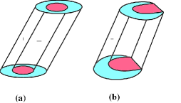
Figure 5: In $(a)$, the worldtube of a $(-)$ energy region is totally surrounded by the worldtube of a $(+)$ energy region. In $(b)$, the $(+)$ energy envelops all but the forward-moving edge of the $(-)$ energy region.

Topologically the $(-)$ energy region here is equivalent to the $(-)$ energy “box” discussed earlier in this section. Therefore, for the null fluid case we can use the same argument to place constraints on the magnitude of the $(-)$ energy density in the interior region and the thickness in its direction of motion. However, here the $(+)$ energy actually need envelop only all but a line of tangency which is transverse to the direction of motion, as depicted in Fig. 5(b). In this case as well, there are no timelike observers who intersect only the $(-)$ energy. As an aside, we point out that the limiting case is when the line of tangency is shrunk to a point which lies along the direction of motion.

III.2.4 Expanding engulfed $(-)$ energy shells

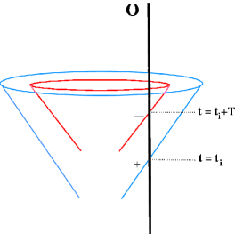
Figure 6: Two spatially concentric, radially expanding $\delta$-function null shells of $(+)$ and $(-)$ energy, created in the past. The worldline of observer $O$ intersects the $(+)$ energy shell at time $t=t_{i}$, and the $(-)$ energy shell a time $T$ later. The vertices of the two light cones, although not shown, are assumed to lie along the same line, which is parallel to $O$.

Consider two spatially concentric, radially expanding $\delta$-function null shells of $(+)$ and $(-)$ energy, which were created at two different times in the past. A stationary observer $O$ is hit first by the $(+)$ shell at $t=t_{i}$, and later by the $(-)$ shell at $t=t_{i}+T$, where $T$ is the separation between the shells in time. This scenario is depicted in Fig. 6. Let the energy density of the $(+)$ shell, as measured by $O$ at time $t_{i}$, be

$$\rho_{+}=\frac{a}{t_{i}^{2}}\,\delta(t-t_{i})\,,$$ (31)

with $a=\,{\rm constant}\,>0$, and the energy density at $t=t_{i}+T$ be

$$\rho_{-}=-\frac{b}{t_{i}^{2}}\,\delta(t-(t_{i}+T))\,,$$ (32)

with $b=\,{\rm constant}\,>0$. The constants $a$ and $b$ are measures of the magnitudes of the energy densities, neglecting the effects of expansion. This scenario can be constrained using the QI’s with a compactly supported sampling function, following the argument given in Sec. III of Ford and Roman (1999).

Choose a compactly supported sampling function with a single maximum centered on $t=t_{i}+T$ (i.e., on the $(-)$ energy shell), with a width $t_{0}$. Substituting Eqs. (31) and  (32) into the QI, we get

$$\hat{\rho} = \int_{-\infty}^{\infty}\,g(t)\,\rho(t)\,dt$$ (33)

$$= \frac{a}{t_{i}^{2}}\,g(t_{i})-\frac{b}{t_{i}^{2}}\,g(t_{i}+T)\,\geq-\frac{C}{{t_{0}}^{4}}\,.$$

If we now choose the width of the sampling function to be $t_{0}=2T$, then $g(t_{i})=0$. For a sampling function with one maximum at $g(t_{i}+T)$, $g(t_{i}+T)\propto 1/{t_{0}}$, so let $g(t_{i}+T)=C_{0}/{t_{0}}=C_{0}/2T$, where $C_{0}$ is a constant whose value depends only on the form of the chosen sampling function (but not on the spacetime dimension, unlike $C$). Therefore we obtain

$$T\leq{\left(\frac{C}{8b\,C_{0}}\right)}^{1/3}\,{t_{i}}^{2/3}\,.$$ (34)

We see that for fixed $t_{i}$, $T$ decreases with increasing $b$, as expected. When $b$ is fixed and for $0<t_{i}\ll T$, we see that $T$ must decrease as $t_{i}$ decreases. (To avoid singularities in the energy densities we do not want to allow $t_{i}\rightarrow 0$, which is why only the later stages of the evolution are illustrated in Fig. 6.) In the limit when $t_{i}\gg T$, for fixed $b$, the bound Eq. (34) becomes very weak.

III.2.5 Separated Expanding Shells of $(+)$ and $(-)$ Energy

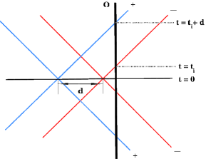
Figure 7: Two contracting shells of $(+)$ and $(-)$ energy reach their maximum densities at $t=0$, and subsequently re-expand. The regions of maximum density are separated by distance $d$. A stationary observer $O$ intersects the $(-)$ energy shell at $t=t_{i}$.

Consider two null fluid $\delta$-function shells of separated $(+)$ and $(-)$ energy which contract and re-expand. The shells reach maximum density at time $t=0$. The spatial locations where the densities become maximum are separated by a distance, $d$. (We ignore any interactions when the shells cross each other.) The evolution of the shells is depicted in Fig. 7. A static observer, $O$, gets hit by each shell twice. The worldline of $O$ crosses the $(-)$ energy shell for a second time at time $t=t_{i}>0$, and crosses the $(+)$ energy shell for the second time at time $t=t_{i}+d$. Note that the diagram is time-symmetric around $t=0$.

The following argument uses only the AWEC to constrain this scenario. As before, let the magnitudes of the energy densities (neglecting the effects of contraction and expansion) be “$a$” for the $(+)$ energy shell and “$b$” for the $(-)$ energy shell, with $a,b$ chosen to be positive constants. If we apply the AWEC to $O$’s worldline, and use the time-symmetry of the diagram, we obtain

$$\int_{-\infty}^{\infty}\,T_{\mu\nu}u^{\mu}u^{\nu}\,dt=\frac{2a}{{(t_{i}+d)}^{2}}-\frac{2b}{t_{i}^{2}}\,\geq 0\,.$$ (35)

The factors of $2$ reflect the fact that $O$ gets hit by each shell twice. If we let $f=a/b$, we can rewrite this as

$$ft_{i}^{2}\geq{(t_{i}+d)}^{2}\,.$$ (36)

The quantities $f$, $t_{i}$, and $d$ are all positive, so we obtain

$$d\leq({\sqrt{f}}-1)\,t_{i}\,.$$ (37)

This implies that $f>1$, and that $f$ must increase as $t_{i}/d$ decreases. In the limit $t_{i}/d\gg 1$, we simply get $f\gtrsim 1$, which is a fairly weak bound.

The bound Eq. (37) becomes more and more stringent as $t_{i}$ decreases. However, it is more realistic to suppose that the shells have a finite thickness $\Delta$. This can be viewed as either the thickness in space at a fixed time, or else the duration in time along $O$’s worldline. Then the above analysis holds so long as $t_{i}>\Delta$, and the best bound, obtained when $t_{i}\approx\Delta$, implies that

$$f\gtrsim\frac{(d+\Delta)^{2}}{\Delta^{2}}\,.$$ (38)

When $d\gg\Delta$, this requires $f\gg 1$, which is a version of the quantum interest phenomenon.

IV Explicit construction of allowed distributions

IV.1 Plane Wave Modes

In the previous section, we discussed $(-)$ energy distributions which were either ruled out or constrained by the AWEC and the QIs. We now give some examples of distributions which can be explicitly constructed from allowed states in quantum field theory, and analyze some of their properties. The class of examples which we will focus on are squeezed vacuum states, which are discussed extensively in quantum optics and which can now be constructed in the laboratory Scully and Zubairy (1997). Our discussion is restricted here to quantized massless and massive minimally coupled scalar fields in flat spacetime, but it could be easily generalized to include the electromagnetic field as well, which is also known to obey the QIs and the AWEC Ford and Roman (1997); Pfenning (2001). The stress tensor for the minimally coupled scalar field is

$$T_{\mu\nu}=\phi_{,\mu}\phi_{,\nu}-{1\over 2}\,\eta_{\mu\nu}\,\left(\phi_{,\alpha}\phi^{,\alpha}\,+m^{2}\,\phi^{2}\right)\,.$$ (39)

The field operator may be expanded in terms of creation and annihilation operators as

$$\phi={\sum_{k}}({a_{k}}{f_{k}}+{a_{k}}^{\dagger}{f_{k}}^{\ast})\,.$$ (40)

For simplicity, we will consider only a single mode state with $t$ and $x$ dependence only, i.e., $f_{k}=f=f(t,x)$. The renormalized expectation values of the energy density, pressure, and flux are then given by

$$T_{00} = Re\,\left[\langle{a^{\dagger}a}\rangle\,(f^{*}_{,t}\,f_{,t}+f^{*}_{,x}\,f_{,x})+\langle{a^{2}}\rangle\,({f_{,t}}^{2}+{f_{,x}}^{2})\right.$$ (41)

$$+\left.m^{2}\,(\langle{a^{\dagger}a}\rangle\,f^{*}f+\langle{a^{2}}\rangle\,f^{2})\right]\,,$$

$$T_{11} = Re\,\left[\langle{a^{\dagger}a}\rangle\,(f^{*}_{,x}\,f_{,x}+f^{*}_{,t}\,f_{,t})+\langle{a^{2}}\rangle\,({f_{,x}}^{2}+{f_{,t}}^{2})\right.$$ (42)

$$-\left.m^{2}\,(\langle{a^{\dagger}a}\rangle\,f^{*}f+\langle{a^{2}}\rangle\,f^{2})\right]\,,$$

$$T_{01} = Re\,\left[\langle{a^{\dagger}a}\rangle\,(f^{*}_{,t}\,f_{,x}+f^{*}_{,x}\,f_{,t})+2\langle{a^{2}}\rangle\,(f_{,t}\,f_{,x})\right]\!\!,$$ (43)

respectively.

Here the mode function will be taken to be a plane wave mode of the form

$$f={i\over\sqrt{2\omega L}}e^{i(kx-\omega t)},$$ (44)

with $\omega=\sqrt{k^{2}+m^{2}}$, and where ${\bf k}=k{\bf\hat{x}}$, and a periodicity of length $L$ has been imposed in the spatial direction, so that $k$ takes on discrete values. We choose the quantum state $|\psi\rangle$ to be a squeezed vacuum state:

$$|\xi\rangle=S(\xi)|0\rangle\,,$$ (45)

where $S(\xi)$ is the “squeeze operator,” and $\xi=r\,e^{i\theta}$ is an arbitrary complex number. In this state,

$$\langle{a^{\dagger}a}\rangle={{\rm sinh}^{2}}r\,,$$ (46)

and

$$\langle{a^{2}}\rangle=-{\rm sinh}r\,{\rm cosh}r\,,$$ (47)

where $r>0$ is the squeeze parameter, and where we have chosen the phase $\theta=0$ Scully and Zubairy (1997). If we substitute Eqs. (44)- (47) into Eqs. (41)-(43), we obtain

$$\!\!\!\!\!\!T_{00} \!\!\!=\!\!\! {\frac{\omega}{L}}\,{\rm sinh}r\left[{\rm sinh}r-{\frac{k^{2}}{\omega^{2}}}\,{\rm cosh}r\,{\rm cos}\,2(kx-\omega t)\right]\!\!\!\,,$$ (48)

$$\!\!\!\!\!\!T_{11} \!\!\!=\!\!\! {\frac{\omega}{L}}\,{\rm sinh}r\left[{\frac{k^{2}}{\omega^{2}}}\,{\rm sinh}r-{\rm cosh}r\,{\rm cos}\,2(kx-\omega t)\right]\!\!\!\,,$$ (49)

$$\!\!\!T_{01} = -{\frac{k}{L}}\,{\rm sinh}r\left[{\rm sinh}r-{\rm cosh}r\,{\rm cos}\,2(kx-\omega t)\right]\,.$$ (50)

Figure 8: The energy density $\rho$ in a single plane wave mode squeezed vacuum state, at constant time $t=0$, as a function of position, $x$. Here $r=0.2$, $\omega=10$, and $m=8$.

The energy density as a function of position at fixed time is plotted in Fig. 8. One obtains a similar graph of energy density as a function of time at fixed position. The energy density oscillates between $(+)$ and $(-)$ values, with the $(+)$ energy always overcompensating the $(-)$ energy.

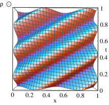
Figure 9: A “top down” view of the energy density, $\rho$ in a single plane wave mode squeezed vacuum state of a massive scalar field, as a function of $x$ and $t$. The energy density increases in the direction perpendicular to the page. The $(-)$ energy is concentrated along spacelike regions. Again $r=0.2$, $\omega=10$, and $m=8$.

For the massive field case it might seem that an observer could ride along with the $(-)$ energy in violation of the QIs. However, since the QIs hold for all quantum states in flat spacetime, we know this cannot be possible. How is this apparent paradox resolved? The energy density as a function of $t$ and $x$ is plotted in Fig. 9. The $(-)$ energy density is concentrated along spacelike regions. So an observer cannot ride along with it. It might appear from this example that the $(-)$ energy is “propagating” along spacelike trajectories. However, a relativistic quantum field theory incorporates causality in its construction. So what is going on? One must remember that these are rather special states which have correlations built into them. These built-in correlations cause the energy density to vary in a manner that looks like acausal propagation. At each point, the energy density is moving in such a way as to create the effect of peaks and troughs of energy that are constant along spacelike lines. This is illustrated in Fig. 10. A useful analogy is the following. Imagine an system of light bulbs with triggering mechanisms and clocks which are arranged in a line. An observer can pre-program each bulb to be triggered at a certain time. This can be done in such a way that another observer who later sees the succession of flashes, and interprets them as causally generating one another, will think that the flashes are propagating faster than light. The correlations of the flash times of the bulbs relative to one another have been causally pre-programmed into the state of the system from the beginning. Another analogy is an Einstein-Podolsky-Rosen state in which two photons are generated in an entangled state such that a measurement of the spin of one photon allows one to determine the spin of the other photon even at spacelike separations. This process cannot be used for superluminal signaling because there is no way to know ahead of time what the spin of the first photon will be before it is measured, which is what one would need to send Morse-code type messages. The two photons are in some sense two parts of one single “object”.

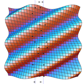
Figure 10: A “top down” view of the energy density, $\rho$ in a single plane wave mode squeezed vacuum state of a massive scalar field, as a function of position (horizontal axis) and time (vertical axis). The energy density increases in the direction out of the page. Null lines are at $45$ degrees. The $(-)$ energy is concentrated along spacelike regions. The arrows indicate the instantaneous direction of flow of the energy. Again $r=0.2$, $\omega=10$, and $m=8$.

Another apparent paradox looms at this point. If the $(-)$ energy is concentrated along spacelike lines, as shown in the figures, then it would seem that a suitably boosted observer could make one of these lines a constant time surface on which the energy density is everywhere negative. However, these surfaces are perpendicular to the observer’s timelike Killing vector (unlike the spacelike surfaces discussed in Fig. 2), and so we know that the energy density integrated over all space must be positive.

In the boosted frame,

$$T^{\prime}_{00}=\gamma^{2}\,T_{00}+2v\,\gamma^{2}\,T_{01}+v^{2}\,\gamma^{2}\,T_{11}\,,$$ (51)

and

$$T^{\prime}_{01}=-v\,\gamma^{2}\,(T_{00}+T_{11})-\gamma^{2}\,(1+v^{2})\,T_{01}\,.$$ (52)

In the boosted frame described above, $T^{\prime}_{01}=0$. A short calculation shows that this is the case when $v=k/\omega$. It is easily shown that this is the value of $v$ which gives ${\bf k}^{\prime}=0$. In this frame

$$T^{\prime}_{00}=\frac{m^{2}\,{{\rm sinh}^{2}}r}{\omega L}={\rm constant}\,>0\,,$$ (53)

so the observer simply sees a constant $(+)$ energy density. This is consistent with the fact that the WEC violations here are weak. We can show this more generally using the results of the Appendix, as follows.

For the massive scalar field in a plane wave squeezed vacuum state, when $T_{00}<0$, what are the conditions that in a boosted frame $T^{\prime}_{00}<0$ as well? Let $\kappa=kx-\omega t$. Since $r>0$ and $\omega>k$, we need $(\omega^{2}/k^{2})\,{\rm tanh}r<{\rm cos}\,2\kappa$ for $T_{00}<0$, which in turn implies that $T_{11}<0$ and $T_{01}>0$, from Eqs. (48)-(50). Therefore we may write

$$|T_{11}| = -T_{11}={\frac{\omega}{L}}\,{\rm sinh^{2}}r\left[{\rm coth}r\,\,{\rm cos}\,2\kappa{-\frac{k^{2}}{\omega^{2}}}\right]\,,$$ (54)

$$|T_{01}| = T_{01}={\frac{k}{L}}\,{\rm sinh^{2}}r\left[{\rm coth}r\,\,{\rm cos}\,2\kappa-1\right]\,.$$ (55)

Note that ${\rm coth}r\,\,{\rm cos}\,2\kappa-({k^{2}}/{\omega^{2}})>{\rm coth}r\,\,{\rm cos}\,2\kappa-1>0$, and $(\omega/L)\,{\rm sinh^{2}}r>(k/L)\,{\rm sinh^{2}}r$, so we have that $|T_{11}|>|T_{01}|$ and $T_{11}<0$. Thus we have an example of Case $1$ of the Appendix, where the necessary and sufficient condition for a strong WEC violation is Eq. (85),

$$T_{00}<\frac{{T_{01}}^{2}}{T_{11}}\,.$$ (56)

Since $T_{11}<0$, this implies $T_{00}T_{11}>{T_{01}}^{2}$. Combining Eqs. (48)-(50), we find

$$T_{00}T_{11}-{T_{01}}^{2}=-(m^{2}/{\omega^{2}L^{2}})\,{\rm cosh}r\,\,{\rm sinh^{3}}r\,\,{\rm cos}\,2\kappa<0\,,$$ (57)

since if $T_{00}<0$, then ${\rm cos}\,2\kappa>0$. Hence the condition, Eq. (85), is violated and the WEC violation by the massive scalar field in the single plane wave mode squeezed vacuum state is weak.

For the massless scalar field, $m=0$ and hence $\omega=|k|$, $T_{00}=T_{11}=-T_{01}$, so this is an example of Case 2.2 of the Appendix, for which the necessary and sufficient condition for strong WEC violation is Eq. (75),

$$|T_{00}|\geq T_{11}+2|T_{01}|\,,$$ (58)

which is marginally satisfied in this case. Hence for the massless scalar field the WEC violation is strong.

IV.2 Wavepackets

We now analyze the distribution of $(+)$ and $(-)$ energy in a wavepacket of the massive scalar field in two-dimensional spacetime. In the mode expansion of the field operator, given in Eq. (40), we will take the $f_{k}$’s to be a complete orthonormal set of wavepacket modes. Let only one single wavepacket mode, $f$, be excited, and take the form of this mode to be Gasiorowicz (1974)

$$f(x,t) = \frac{\alpha^{1/4}}{2^{3/4}\,\pi^{1/4}\,\sqrt{\omega_{0}}}\,{\left(1+\frac{\sigma}{4\,\alpha\,\omega_{0}}\right)}^{-1/2}$$ (59)

$$\times e^{i\,(k_{0}\,x-\omega_{0}\,t)}\,e^{-{{(x-v_{g}\,t)}^{2}}/4\,(\alpha+i\,\sigma\,t)}\,,$$

where $\omega_{0}=\sqrt{k_{0}^{2}+m^{2}}$,

$$v_{g}={\left(\frac{d\omega}{dk}\right)}_{k_{0}}=\frac{k_{0}}{\omega_{0}}\,,$$ (60)

is the group velocity of the packet, and where

$$\sigma=\frac{1}{2}\,{\left(\frac{d^{2}\omega}{dk^{2}}\right)}_{k_{0}}=\frac{m^{2}}{2\omega_{0}^{3}}\,.$$ (61)

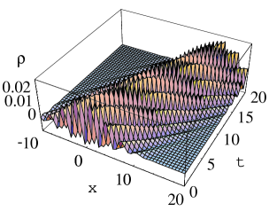
Figure 11: The energy density $\rho$ as a function of $x$ and $t$ for a massive scalar field in a wavepacket mode squeezed vacuum state. The peak of the packet follows a timelike trajectory. The negative energy is concentrated along the spacelike troughs. Here $r=0.2$, $k_{0}=0.6$, $m=8$ and $\alpha=20/k_{0}^{2}$.

The packet is sharply peaked around $k_{0}$ in momentum space with spread $1/\sqrt{\alpha}$, where we assume that $\alpha\gg 1$. With these assumptions the wavepacket has unit Klein-Gordon norm. As before take the quantum state to be a squeezed vacuum state, and substitute Eq. (59) into Eq. (41). A tedious calculation then yields a rather long expression for $T_{00}$ which we do not reproduce here. A plot of $\rho=T_{00}$ as a function of $t$ and $x$ is shown in Fig. 11. Note that the peak of the wavepacket moves along a timelike trajectory with the group velocity, $d\omega/dk$, whereas the individual components move with the phase velocity, $\omega/k$. As in the plane wave case for the massive scalar field, the negative energy is concentrated along spacelike regions.

V The AWEC along geodesic segments

In this section, we will depart somewhat from the principal topic of this paper and discuss some of the limitations of the AWEC. We illustrate why the AWEC integral must be taken along a complete geodesic path. We will also have an opportunity to explore examples of both strong and weak violations of the WEC.

V.1 A Counterexample to the AWEC for Piecewise Geodesics

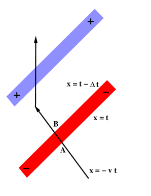
Figure 12: An observer on a piecewise geodesic path moves through separated regions of $(+)$ and $(-)$ energy. The observer moves through the $(-)$ energy on the path $x=-vt$. The lower boundary of the $(-)$ energy region is the line $x=t$ and its upper boundary is the line $x=t-\Delta t$.

In this subsection we wish to show that the averaged weak energy condition does not hold, even in Minkowski spacetime, if one integrates the energy density along a piecewise geodesic path, as opposed to a true geodesic. Consider an energy distribution with the null fluid form for the stress tensor, Eq. (24). Suppose that there are separated $(+)$ and $(-)$ energy regions, both moving to the right, as illustrated in Fig. 12. For the purposes of our example, we may take the energy density to be constant within each region, so that $\rho=\rho_{+}$ in the $(+)$ energy region and $\rho=\rho_{-}$ in the $(-)$ energy region. Further require that both pulses last for the same time interval $\Delta t$ as measured in the laboratory frame. This means that we must have

$$\rho_{+}>|\rho_{-}|$$ (62)

in order that there be net $(+)$ energy.

Now consider an observer moving to the left with speed $v$, and hence with four-velocity $u^{\mu}=\gamma(1,-v,0,0)$, where $\gamma=1/\sqrt{1-v^{2}}$. The energy density in the frame of this observer is

$$T^{\mu\nu}u_{\mu}u_{\nu}=\rho\,\gamma^{2}\,(1+v)^{2}\,.$$ (63)

Further suppose that this observer moves along the piecewise geodesic worldline depicted in Fig. 12. The observer first moves at speed $v$ through $(-)$ energy, and then is at rest when the $(+)$ energy passes by. The path of the observer in the $(-)$ energy can be taken to be given by $x=-vt$, and the boundaries of the $(-)$ energy to be the lines $x=t$ and $x=t-\Delta t$. The observer enters the $(-)$  energy at point $A$, where $x=t=0$. Let $T$ be the coordinate time required to traverse the $(-)$ energy region. At point $B$, we have $x=-vT=T-\Delta t$. Hence the proper time which the observer spends in the $(-)$ energy is

$$\tau=\frac{T}{\gamma}=\frac{\Delta t}{\gamma(1+v)}\,.$$ (64)

The integrated energy density along this observer’s worldline is

$$\int T^{\mu\nu}u_{\mu}u_{\nu}d\tau = \rho_{+}\,\Delta t+\rho_{-}\,\tau\,\gamma^{2}\,(1+v)^{2}$$ (65)

$$= \Delta t\left(\rho_{+}-|\rho_{-}|\,\sqrt{\frac{1+v}{1-v}}\right)\,.$$

So long as $\rho_{-}\not=0$, we can find a $v$ which makes this expression negative. The piecewise nature of the worldline allows the $(-)$ energy to be enhanced in magnitude by the Doppler shift factor $\sqrt{(1+v)/(1-v)}$, while the $(+)$ energy is unchanged.

V.2 Violations of the Difference AWEC

The AWEC in its simple form need not hold inside of a cavity, if there is negative Casimir energy density. In this case, an observer can sit in constant negative energy density for an infinite amount of proper time. However, the difference between the energy density in an arbitrary quantum state and in the Casimir vacuum does satisfy the AWEC. More generally, this difference satisfies quantum inequalities, as was discussed in Ref. Ford and Roman (1995); Mitch98 . These “difference inequalities” reduce to the “difference AWEC” in the limit of long sampling times. The latter is the statement that the integral of the difference in energy densities is non-negative when integrated over the worldline of an observer at rest within the cavity. However, just as it is possible to temporarily suppress the local energy density below zero in empty Minkowski spacetime, it is possible to find quantum states in which the local energy density is more negative than in the Casimir vacuum state. The question which we wish to address in this subsection is the following: Is it possible for a moving observer to pass through a cavity in such a way as to see a net negative integrated energy from a quantum field confined within the cavity? Here we are concerned only with the stress tensor of the quantum field, and are ignoring any contributions from the walls of the cavity itself.

Consider a massless scalar field confined between reflecting boundaries located at $x=0$ and at $x=L$, and a geodesic observer moving at speed $v$ in the positive $x$-direction. The four velocity of the observer is $u^{\mu}=\gamma(1,v,0,0)$ and the energy density in this observer’s rest frame is

$$\rho=T^{\mu\nu}\,u_{\mu}\,u_{\nu}\,.$$ (66)

Here $T^{\mu\nu}$ is understood to be the difference in the expectation values of the stress tensor operator in a given quantum state and in the Casimir vacuum. Let the quantum state be one in which a single mode, with mode function $f$, is excited. Then the components of $T^{\mu\nu}$ are given by the same expressions that hold for the normal-ordered stress tensor in Minkowski spacetime, namely Eqs. (41),  (42), and  (43). We may use these expressions to write $\rho$ as

$$\rho = 2{\rm Re}\{(\gamma^{2}-\frac{1}{2})\,[|f_{,t}|^{2}\langle a^{\dagger}a\rangle+(f_{,t})^{2}\langle a^{2}\rangle]$$ (67)

$$+ (v^{2}\gamma^{2}+\frac{1}{2})\,[|f_{,x}|^{2}\langle a^{\dagger}a\rangle+(f_{,x})^{2}\langle a^{2}\rangle]$$

$$+ v\gamma^{2}[(f_{,t}^{*}f_{,x}+f_{,x}^{*}f_{,t})\langle a^{\dagger}a\rangle+2f_{,t}f_{,x}\langle a^{2}\rangle]\}\,.$$

We take the mode function to be that of a standing wave which vanishes on the walls of the cavity and has no dependence upon the transverse directions:

$$f=f(t,x)=A\,\sin\omega x\,{\rm e}^{-i\omega t}\,.$$ (68)

Note that the standing wave modes must satisfy

$$\omega=\frac{\pi n}{L}\,,\quad n=1,2,3,\cdots\,.$$ (69)

We wish to examine the integrated energy density along this observer’s worldline. Here it is assumed that there are no particles outside of the cavity, so the difference in energy densities is nonzero only inside of the cavity. The integrated energy density difference then becomes

$${\cal E}=\int\rho\,d\tau=\frac{1}{\gamma}\,\int_{t_{0}}^{t_{0}+\Delta t}\rho\,dt\,,$$ (70)

where $\Delta t=L/v$ is the coordinate time required to traverse the cavity, and $t=t_{0}$ is the time at which the observer enters. Let the quantum state be the single mode squeezed vacuum state discussed in Sec. IV. We can now use Eqs. (67),  (68),  (46), and  (47) to write

$${\cal E} = \frac{A^{2}\,\omega\,\sinh r}{4\,\sqrt{1-v^{2}}}\;\Biggl{\{}\cosh r\,\biggl{[}2\sin(2\omega t_{0})$$ (71)

$$- (1+v)\sin\{2[(1+v)\Delta t+t_{0}]\omega\}$$

$$- (1-v)\sin\{2[(1-v)\Delta t+t_{0}]\omega\}\biggr{]}$$

$$+ 4(1+v^{2})\,\omega\,\Delta t\,\sinh r\Biggr{\}}\,.$$

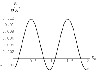
Figure 13: ${\cal E}/\omega^{2}A^{2}$ is plotted as a function of the entrance time $t_{0}$ for the case that $r=0.03$ and $v=0.9$.

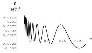
Figure 14: ${\cal E}/\omega^{2}A^{2}$ is plotted as a function of the observer’s speed $v$ for the case that $r=0.03$ and $t_{0}=0$.

Let the excited mode be the lowest frequency, $n=1$, mode. It is possible to arrange for the observer to see net negative integrated energy for selected values of the parameters $r$, $v$ and $t_{0}$. For example, ${\cal E}$ is plotted in Fig. 13 as a function of $t_{0}$ for $r=0.03$ and $v=0.9$. The result can be either positive or negative. The cavity contains net positive energy, but with oscillatory pockets of negative energy density. An observer who enters the cavity at certain times during the cycle will manage to see net negative energy, whereas one who enters at other times may see net positive energy. It is also of interest to look at ${\cal E}$ as a function of $v$ for fixed $r$ and $t_{0}$. This is illustrated in Fig. 14, where $r=0.03$ and $t_{0}=0$. Note that for smaller values of $v$, ${\cal E}>0$, whereas larger values of $v$ allow the observer to see net negative energy, ${\cal E}<0$. If the observer spends too long in the cavity, the energy oscillations cause the time-integrated energy to be positive, but a speedier observer can manage to catch net negative energy. Again it is important to emphasize that this net negative energy represents only the contribution of the quantum field in the cavity and not of the walls themselves. For any realistic cavity, it is overwhelmingly likely that the AWEC integral including the walls’ rest mass energy will be positive.

V.3 Strong and Weak Violations of the WEC in a Cavity

We have seen in Sec. IV that the scalar field in a single mode squeezed vacuum state can violate the WEC. For a travelling wave mode, it was shown that the violation is always weak for the massive field and always strong for the massless field. The cavity discussed in the previous subsection allows us to give an example where both strong and weak violations occur simultaneously in different regions of space. Again take a massless scalar field in the cavity to be in a squeezed vacuum state for the mode given in Eq. (68). The energy density and pressure are equal and given by

$$T_{00}=T_{11}=A^{2}\,\omega^{2}\,\sinh r[\sinh r-\cos 2\omega x\,\cos 2\omega t\,\cosh r]\,,$$ (72)

The flux is given by

$$T_{01}=A^{2}\,\omega^{2}\,\sinh r\,\cosh r\,\sin 2\omega x\,\sin 2\omega t\,.$$ (73)

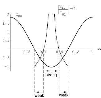
Figure 15: The regions of strong and weak violation of the WEC are shown. The energy density and the parameter $|T_{11}/T_{01}|-1$ for the $n=1$ mode are plotted as functions of position in the cavity at time $t=3/8$. Here units in which $L=1$ are used, and we have set $A=1$ and $r=0.2$.

Let us suppose that we are at a point at which the WEC is violated, so $T_{00}<0$, or $\cos 2\omega x\,\cos 2\omega t>\tanh r$. If $|T_{11}|>|T_{01}|$, we are in Case 1 of the Appendix, in which the necessary and sufficient condition for a strong violation is Eq. (85). However, when $T_{00}=T_{11}<0$, this condition always holds if $|T_{11}|>|T_{01}|$. On the other hand, suppose that $|T_{11}|\leq|T_{01}|$. Then we are in Case 2.2 of the Appendix, and the necessary and sufficient condition for a strong violation is Eq. (75). In summary, in the cavity all WEC violations are strong if $|T_{11}|\geq|T_{01}|$ and weak if $|T_{11}|<|T_{01}|$. It is possible to find both types of violation, as is illustrated in Fig. 15. In this example, the WEC violation is strong in the middle of the $(-)$ energy region, and weak nearer to its edges.

VI Summary and future directions

Let us summarize some of the results obtained in this paper, as well as some of the unanswered questions which this investigation has raised. We have given some explicit examples of spacetime averaged quantum inequalities in two-dimensional spacetime. However, the problem of finding similar results in four-dimensional spacetime is unsolved. We have used the AWEC and QIs to rule out or limit some particular model distributions of $(-)$  energy. In particular, the “cap the cone” argument given in Sec. III.1.1 shows that one cannot have a piece of $(-)$  energy separated from rigidly moving positive energy. We were able to give quantitative restrictions on other possible distributions. We also gave some explicit examples of allowed distributions. However, much more work needs to be done to narrow the gap between distributions which can be ruled out and those which are definitely allowed. As part of our investigation, we have introduced the distinction between strong and weak violations of the WEC, which is likely to prove useful in future work on this subject. We have also tested the limits of the AWEC and provided counterexamples to the AWEC along piecewise geodesics and to the difference AWEC for observers who pass through a cavity. These types of counterexamples are useful for understanding more clearly just which conditions can be used to constrain spatial distributions of $(-)$ energy.

Future work in this area will involve a search for a more systematic ways to use information from worldline integrals to reconstruct or constrain spatial and spacetime distributions of $(-)$  energy. It will also involve the construction of additional explicit examples. It is especially interesting to see how far one can go in four spacetime dimensions toward having separated regions of $(+)$  and $(-)$  energy.

*

Appendix A Strong and weak violations of the weak energy condition

If an observer measures negative energy at a point, must others measure it as negative too? If all observers measure the energy at a point to be negative, we say that we have a strong violation of the weak energy condition at that point. If only some do, we say that we have a weak violation. Suppose that an observer measures negative energy; i.e., $T_{00}<0$ in the observer’s rest frame. What are the conditions on the components of $T_{\mu\nu}$ so that there is a strong violation of the weak energy condition? We consider the question in two-dimensional flat spacetime.

Under a Lorentz transformation, we have

$$T^{\prime}_{00}=\gamma^{2}(T_{00}+2vT_{01}+v^{2}T_{11}),$$ (74)

where $v$ and $\gamma$ are the usual boost and Lorentz factors, and $v$ obeys $-1<v<1$. Assuming that $T_{00}<0$, we want the necessary and sufficient condition that $T^{\prime}_{00}<0$ as well, no matter what the value of $v$. This occurs trivially, for instance, if both $T_{01}$ and $T_{11}$ are zero. We call this the trivial case.

In nontrivial cases, the condition

$$|T_{00}|\geq T_{11}+2|T_{01}|$$ (75)

is necessary for $T^{\prime}_{00}<0$, $\forall v$. In order to see this, suppose that the condition is violated. One of $T_{01}$ or $T_{11}$ cannot be zero, so we must have

$$-T_{00}<T_{11}+2|T_{01}|.$$ (76)

This implies that for sufficiently small $\epsilon>0$, we have

$$-T_{00}<(T_{11}-\epsilon/2)+2(|T_{01}|-\epsilon/4).$$ (77)

Now, there must exist some $v_{1}>0$ such that

$$v^{2}T_{11}>T_{11}-\epsilon/2,\quad\forall|v|>v_{1},$$ (78)

and some $v_{2}>0$ such that

$$|v||T_{01}|>|T_{01}|-\epsilon/4,\quad\forall|v|>v_{2}.$$ (79)

Putting these together, we see that

$$T_{00}+v^{2}T_{11}+2|v||T_{01}|>0,\quad\forall v>\max(v_{1},v_{2}).$$ (80)

We choose $v$ to be $(+)$ or $(-)$ depending on whether $T_{01}$ is $(+)$ or $(-)$. This gives us

$$T^{\prime}_{00}=T_{00}+v^{2}T_{11}+2vT_{01}>0,\text{\ for some\ }v.$$ (81)

In other words, we do not have a strong violation of the weak energy condition.

In order to discuss sufficient conditions, there are two cases we need to consider:

1. $T_{11}<0$ and $|T_{01}|<|T_{11}|$

2. Other

We look at the second case first. In this case, condition 75 is sufficient as well. To see this, we need to look at two subcases:

Case 2.1, $T_{11}\geq 0$: Since $|v|<1$, we have $T_{11}\geq v^{2}T_{11}$ and $2|T_{01}|\geq 2|v||T_{01}|\geq 2vT_{01}$, with equality holding in each instance only if both sides are zero. Since we are looking at nontrivial cases, at least one of $T_{11}$ and $T_{01}$ is non-zero. Then condition 75 implies that

$$-T_{00}\geq T_{11}+2|T_{01}|>v^{2}T_{11}+2vT_{01},\quad\forall v.$$ (82)

In other words

$$T^{\prime}_{00}=T_{00}+v^{2}T_{11}+2vT_{01}<0,\quad\forall v.$$ (83)

Case 2.2, $T_{11}<0$ and $|T_{01}|\geq|T_{11}|$: We must have $T_{01}\neq 0$ here, otherwise we get the trivial case. Define the function $f(v)$ by

$$f(v)\equiv T_{00}+2vT_{10}+v^{2}T_{11},\quad-1\leq v\leq 1.$$ (84)

The graph of this function, under the imposed conditions, is a downward pointing parabola whose extremum $v_{\text{ext}}=-T_{10}/T_{11}$ lies outside the domain. In order to have $f(v)<0$ for all $v$, we need to ensure that the higher of $f(1)$ and $f(-1)$ is nonpositive. When $T_{01}>0$, the higher of the two is $f(1)$ and when $T_{01}<0$, the higher point is $f(-1)$. Now, condition 75 reduces to $f(1)\leq 0$ when $T_{01}>0$ and to $f(-1)\leq 0$ when $T_{01}<0$, giving us precisely what we want.

Case 1, $T_{11}<0$ and $|T_{01}|<|T_{11}|$: Condition 75 is still necessary here, but it is not sufficient. If, for example $T_{00}=-0.0001$, $T_{11}=-4$ and $T_{01}=1$, it is easy to check that the condition holds. Yet, for $v=1/200$ we get a positive value for $T^{\prime}_{00}$. In order to derive the correct condition, consider the function $f(v)$ defined above. In this case, the extremum, $v_{\text{ext}}=-T_{10}/T_{11}$, lies inside the domain of the function and the condition to impose is $f(v_{\text{ext}})<0$. Therefore, the necessary and sufficient condition in this case is

$$T_{00}<\frac{T_{01}^{2}}{T_{11}}.$$ (85)

This is a stronger condition than 75, in that it implies that condition but is not implied by it.

The results of this appendix may be summarized in the following theorem:

Theorem: Let $T_{\mu\nu}$ be the stress energy tensor in a two -dimensional flat spacetime. Suppose that at some point $P$ we have a negative energy density, i.e., $T_{00}<0$. The conditions that the energy density $T^{\prime}_{00}$ in an arbitrary frame is also negative are as follows:

1. If $T_{01}=0$ and $T_{11}=0$, then $T^{\prime}_{00}$ is automatically negative.

2. If $T_{11}<0$ and $|T_{01}|<|T_{11}|$, then

   $$|T_{00}|\geq T_{11}+2|T_{01}|$$ (86)

   is necessary but not sufficient for $T^{\prime}_{00}<0$. The condition

   $$T_{00}<\frac{T_{01}^{2}}{T_{11}}$$ (87)

   is necessary and sufficient for $T^{\prime}_{00}<0$.

3. In all other cases

   $$|T_{00}|\geq T_{11}+2|T_{01}|$$ (88)

   is necessary and sufficient for $T^{\prime}_{00}<0$.

These results may theoretically be applied to the four-dimensional case as well. Suppose that we have a violation of the weak energy condition in the rest frame of an observer. Does an observer boosted in a spatial direction $\vec{x}$ also measure negative energy? We may rotate coordinates so that $\vec{x}$ points in the new x-direction ($T_{00}$ will be unaffected by the transformation), then apply the conditions of this section to the $T_{00}$, $T_{01}$ and $T_{11}$ components in the rotated coordinates.