Testing Scalar-Tensor Gravity Using Space Gravitational-Wave Interferometers
Abstract
We calculate the bounds which could be placed on scalar-tensor theories of gravity of the Jordan, Fierz, Brans and Dicke type by measurements of gravitational waveforms from neutron stars (NS) spiralling into massive black holes (MBH) using LISA, the proposed space laser interferometric observatory. Such observations may yield significantly more stringent bounds on the Brans-Dicke coupling parameter than are achievable from solar system or binary pulsar measurements. For NS-MBH inspirals, dipole gravitational radiation modifies the inspiral and generates an additional contribution to the phase evolution of the emitted gravitational waveform. Bounds on can therefore be found by using the technique of matched filtering. We compute the Fisher information matrix for a waveform accurate to second post-Newtonian order, including the effect of dipole radiation, filtered using a currently modeled noise curve for LISA, and determine the bounds on for several different NS-MBH canonical systems. For example, observations of a NS inspiralling to a MBH with a signal-to-noise ratio of 10 could yield a bound of , substantially greater than the current experimental bound of .
I Introduction and Summary
The observation of gravitational waves from inspiralling compact binaries is expected to provide an excellent testbed for theories of gravity alternative to general relativity (GR) (see [2] for a review). In earlier work [3], we have shown that the measurement of gravitational waves from neutron star (NS) - black hole (BH) mergers by ground-based detectors such as the Laser Interferometric Gravitational-Wave Observatory (LIGO) could bound the strength of a scalar field in scalar-tensor theories of gravity. The bounds estimated in [3] were potentially better than the solar system bounds that were in force at the time (1994), but are no longer competitive with bounds that have improved through the use of Very Long Baseline Interferometry (VLBI) to measure the deflection of light by the sun.
In this paper, we analyze potential bounds on scalar-tensor theory made possible by plans for space-based gravitational-wave observatories such as the Laser Interferometer Space Antenna (LISA), a proposed project of the National Aeronautics and Space Administration (NASA) and the European Space Agency (ESA) [4]. We show that the detection of NS inspirals into massive black holes (MBH) by LISA may provide an opportunity to place significantly more stringent bounds on scalar-tensor theory than current solar-system or binary-pulsar bounds or those achievable by an Earth-based detector.
Space-based interferometers are being designed to detect gravitational-wave signals in a lower frequency band than ground-based detectors such as LIGO, GEO, VIRGO, and TAMA, which measure waves from approximately 10 Hz to Hz. The latter interferometers are expected to detect waves from low-mass inspiralling compact binaries (masses ). LISA is being designed to detect inspirals and mergers of massive black holes (MBH) with masses of , among other potential sources [4]. Mergers of such high-mass objects will produce waves in LISA’s proposed sensitive band of frequencies between Hz and Hz.
The inspiral of such binary systems is driven by gravitational radiation reaction, which imprints onto the phase and amplitude of the emitted gravitational waves information about the masses and spins of the orbiting bodies, about the orbital elements and their evolution, and about the theory of gravity that is in force. Because broad-band interferometric detectors are particularly sensitive to the phasing of the waves, accurate determinations of system and theoretical parameters are possible [5].
The simplest version of scalar-tensor gravity is that studied by Jordan, Fierz, Brans and Dicke, commonly known as Brans-Dicke (BD) theory [6]. In BD, a scalar gravitational field is postulated in addition to the spacetime metric , with an effective strength inversely proportional to a coupling parameter . In BD, is assumed to be a fixed constant. (Generalized scalar-tensor theories that are currently popular byproducts of string theory and other unification schemes treat as a function of .) As , the effect of the scalar field tends to zero and BD GR. Current experimental bounds on from measurements of light bending place (for a review see [7]; for recent light bending measurements, see [8]).
The details of the behavior of compact binaries in scalar-tensor gravity have been worked out by Eardley [9], Will [10], Zaglauer [11] and Damour and Esposito-Farèse [12]. The chief difference between general relativity and scalar-tensor gravity is the existence, in the latter, of dipole gravitational radiation. In general relativity, for slowly moving systems, the leading multipolar contribution to gravitational radiation is quadrupolar, with the result that the dominant radiation-reaction effects are at order relative to Newtonian gravity, where is the orbital velocity. The rate, due to quadrupole radiation in GR, at which a binary system loses energy is given by
| (1) |
where , , and represent the orbital separation, relative orbital velocity, and radial velocity, respectively. We use units in which . The quantities and are the reduced mass parameter and total mass, respectively, given by , and . In BD, this formula is modified by corrections to the coefficients of (BD also predicts monopole radiation, but in binary systems it contributes only to these corrections).
The important modification in BD is the additional energy loss caused by dipole radiation. By analogy with electrodynamics, dipole radiation is a effect, potentially much stronger than quadrupole radiation. However, in scalar-tensor theories, the gravitational “dipole moment” is governed by the difference between the bodies, where is a measure of the self-gravitational binding energy per unit rest mass of each body. Technically, is the “sensitivity” of the total mass of the body to variations in the background value of Newton’s constant, which, in these theories, is a function of the scalar field:
| (2) |
where is the effective Newtonian constant at the star and the subscript denotes holding baryon number fixed. The energy loss caused by dipole radiation is given by
| (3) |
valid to first order in , where .
In BD, the sensitivity of a black hole is always , while the sensitivity of a neutron star varies with the equation of state and mass. For example, for a NS with a stiff equation of state, and for a NS with a soft equation of state. A more detailed discussion of neutron star sensitivities can be found in [11, 13] in the context of Brans-Dicke theory, and in [12] in the context of general scalar-tensor gravity. For white dwarfs, .
Ironically, binary black-hole systems are not at all promising for studying dipole gravitational radiation because , a consequence of the no-hair theorems for black holes. Essentially they radiate away any scalar field, so that a binary black hole system in scalar-tensor theory behaves as if GR were valid (see [3] for further discussion). Similarly, binary neutron star systems, such as the Hulse-Taylor binary pulsar PSR 1913+16 and similar systems, are also not effective testing grounds for dipole radiation [11]. This is because neutron star masses tend to cluster around the Chandrasekhar mass of , and the sensitivity of neutron stars is not a strong function of mass for a given equation of state. Hence in systems like the binary pulsar, dipole radiation is naturally suppressed by symmetry, and the bound achievable cannot compete with those from the solar system [14]. Thus the most promising systems are mixed: BH-NS, BH-WD, or NS-WD.
While a leading scientific motivation for LISA is detection of waves from the merger of binary massive black holes in the centers of galaxies at cosmological distances, LISA will also be able to study waves from the inspiral of low-mass compact objects (black holes, neutron stars, white dwarfs) into massive black holes in galaxies and globular clusters. The orbits of these inspiralling bodies are expected to be complex: possibly highly eccentric because the bodies will have been sent toward the hole by gravitational scattering from stars in the surrounding cluster; possibly strongly perturbed by the surrounding stars each time the body passes through its apholion; possibly dragged in a precessing orbit by the Lens-Thirring effect of a rapidly rotating hole. Analysing the gravitational waves from such orbits will be a challenging task.
However, to study the potential for testing scalar-tensor gravity, we will make a drastic simplification of the problem: we will assume that the compact body spirals toward a non-rotating hole on an adiabatically shrinking circular orbit, up to the innermost stable circular orbit (ISCO) of the black hole, whereupon the body plunges across the horizon on a short timescale. We will assume that the waves from such a quasi-circular orbit can be studied for up to a year using LISA.
With these assumptions, one can make a crude estimate of the bounds on scalar-tensor theory that could be possible. The idea is to use matched filtering of a theoretical template waveform against the output of the detector. A “match” is a signal whose total accumulated phase over the integration time of the experiment matches that of the template within a number of radians set by the time resolution of the instrument and the relevant frequency. The accumulated phase is given by
| (4) |
where is the gravitational-wave frequency (twice the orbital frequency), and the subscripts “i” and “f” denote the values at the beginning and end of the integration. The evolution of the frequency is given by
| (5) |
where is the “chirp” mass, and . The leading term in Eq. (5) is the contribution of quadrupole radiation damping from Eq. (1). The second term is the contribution of dipole radiation damping [Eq. (3)], where . Integrating Eq. (5) using only the leading term, we obtain approximate initial and final frequencies corresponding to an observation period leading up to the innermost stable circular orbit whose gravitational-wave frequency is ; Eq. (5) then yields the dipole contribution to the phase given by . For a neutron star and a black hole, the frequency at the ISCO is less than 0.5 Hz, while, with five million kilometer arm lengths, the minimum time resolution for LISA is of order 30 seconds, hence the minimum phase resolution for waves from such a black hole is of order 100 radians. Demanding that the accumulated phase offset due to dipole radiation reaction be less than this resolution leads to the crude bound on given by
| (6) |
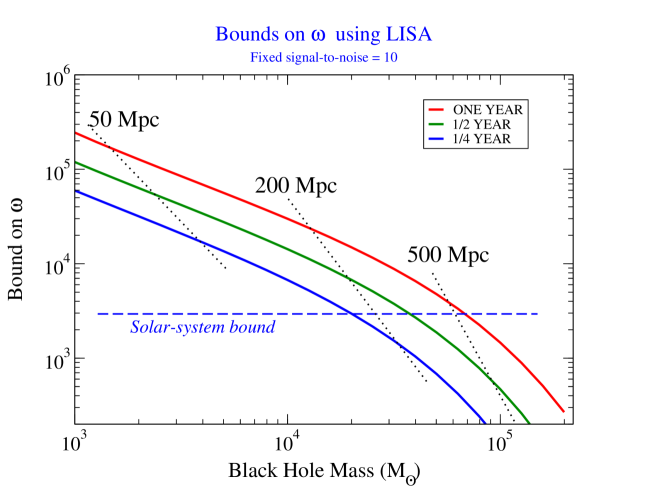
We confirm this crude estimate with detailed calculations using matched filtering to estimate the parameters of such NS-MBH inspiralling systems, and employing current proposals for the instrumental noise curve for LISA together with an estimate for confusion noise caused by a background of galactic white dwarf binaries. The results are displayed in Fig. 1. Shown are the bounds achievable for neutron stars inspiralling into black holes with masses between 1000 and 200,000 , and for integration times of one year, 1/2 year and 1/4 year leading up to the innermost stable orbit. Notice that the bound decreases in almost inverse proportion to black hole mass in agreement with our crude estimate; this is a result of the lower intrinsic frequencies of high mass systems, and the consequent accumulation of fewer cycles in the relevant integration time, leading to less ability to separate out the dipole effects from quadrupole phasing. Notice also that, for a given mass, the bound scales almost linearly with integration time, again in agreement with our crude estimate. Throughout, we assume for concreteness a maximum (and thus) pessimistic value for the sensitivity of the neutron star, so that . If were as low as 0.1, the bounds would increase by . For white dwarf inspirals (), the bounds would be larger by , provided that , so that the white dwarf reaches the ISCO without tidal disruption. For , integration must be cut off as many as a dozen days before the ISCO, with a consequent loss of sensitivity, so that for a black hole, white dwarf inspiral leads to almost the same bound as does NS inspiral.
The remainder of the paper is devoted to details of the method and calculations. In Sec. II we summarize the basic method of parameter estimation using matched filtering; this method is based on foundations laid for gravitational-wave detection by Finn and Chernoff [15] and Cutler and Flanagan [16], and applied to specific parameter estimation problems for inspiralling systems by Will and Poisson [3, 17, 18]. In Sec. III we apply the method specifically to observations by space interferometers. First we consider LISA. Then we we apply the method to a hypothetical follow-on to the LISA mission (which we call SuperLISA), whose sensitive band would lie between that of LISA and the ground based interferometers. The results are discussed in Sec. IV
II Estimating binary system parameters using matched filtering
It is expected that laser interferometric observatories, whether ground-based or space-based, will endeavor to detect gravitational waves from binary inspirals using a technique known as matched filtering [5], wherein a template consisting of a theoretical gravitational waveform is compared to the detector output. The template that is a match with an actual signal present with the noise will show a strong correlation with the detector output and thereby will “filter” a signal out of background noise. The template is represented by , related to the spatial components of the radiative metric perturbation far from the source. In the so-called “restricted post-Newtonian approximation” for an inspiral orbit that is quasi-circular (that is, circular apart from the adiabatic decrease in separation), we approximate , where is a slowly varying wave amplitude; it depends on the wave polarization, the location of the source on the sky relative to the detector, the detector orientation, and the distance to the source; is the phasing of the wave, which is a function of the evolving orbital frequency; and denotes the real part. The wave amplitude is considered only to Newtonian order, i.e. given by the lowest-order, quadrupole approximation, because the process of matched-filtering is rather insensitive to changes in the amplitude of the wave. Matched filtering is very sensitive to the phasing of the wave, however, and thus is taken to the highest post-Newtonian order possible. The Fourier transform of using the stationary phase approximation is given by
| (7) |
where is the largest frequency for which the wave can be described by the restricted post-Newtonian approximation. For inspiral into black holes, this is often taken to correspond to waves emitted at the innermost stable orbit (ISCO) before the bodies plunge toward each other and merge. In the limit where one mass is much smaller than the other, this frequency is given by
| (8) |
All the relevant factors related to the polarization of the wave, distance to the source, and its position on the sky are included in the amplitude . After averaging over all angles, we obtain
| (9) |
where is the “luminosity” distance of the source,
Whereas the amplitude is calculated to Newtonian order, the phase includes higher post-Newtonian corrections. To Newtonian order in general relativity, is given by
| (10) |
where and is formally defined as the phase of the wave at the time of coalescence, .
In BD, for quasi-circular orbits, this formula is modified in two ways. (1) To leading order, the modifications of quadrupole and monopole radiation can be subsumed in the simple replacement of the GR chirp mass in Eqs. (9) and (10) by an effective chirp mass given by
| (11) |
where
| (12) | |||||
| (13) |
and where and are the sensitivities of the two bodies. (2) Via the energy loss in Eq. (3), dipole radiation introduces another term in the phase , so that Eq. (10) now reads
| (14) |
where the parameter is given by
| (15) |
As , . For more details on the gravitational waveform in BD, see [3]. Because we assume a priori that , we shall approximate . We further add to the phasing formula the PN term and the 1.5 PN “tail” term of general relativity; they serve the useful purpose in the matched filter of breaking the degeneracies among the various parameters through their different frequency dependences. While not strictly correct in BD, they are individually valid up to corrections of order . Thus we adopt the phasing [3]
| (17) | |||||
where the third and fourth terms inside the square brackets are the PN and 1.5PN terms, respectively. Notice that, because , the dipole term is compared to the quadrupole term, as expected.
By maximizing the correlation between a template waveform that depends on a set of parameters (for example, the chirp mass ) and a measured signal, matched filtering provides a natural way to estimate the parameters of the signal and their errors (for discussion, see [15, 16]). With a given detector noise spectrum one defines the inner product between two signals and by
| (18) |
where and are the Fourier transforms of the gravitational waveforms . The signal-to-noise ratio (SNR) for a given is given by
| (19) |
One then defines the “Fisher information matrix” with components given by
| (20) |
An estimate of the rms error, , in measuring the parameter can then be calculated, in the limit of large SNR, by taking the square root of the diagonal elements of the inverse of the Fisher matrix,
| (21) |
The correlation coefficients between two parameters and are given by
| (22) |
In our calculations, the parameters to be estimated will be , , , , and , where , and is a fiducial frequency characteristic of the detector noise spectrum. We follow the method used in [3]: combining Eqs. (7) and (17) and calculating the partial derivatives for the five listed parameters, we construct the Fisher information matrix using Eqs. (18) and (20). For simplicity, we set equal to its nominal GR value of zero in all information matrix expressions. We then invert the information matrix and evaluate the errors in the five parameters, along with the correlation coefficients between , and . Since the nominal value of is zero (), the error on it translates into a lower bound on . Results are calculated for the canonical neutron star mass of , and for various values of the black hole mass.
III Bounds on scalar-tensor gravity from space-based interferometers
A LISA-type interferometer
We consider space-based interferometers of the proposed LISA type, with a sensitive bandwidth between and Hz, typical integration times up to one year, and an expected noise curve which can be expressed in terms of an overall amplitude , and a function of the ratio :
| (23) |
Including the LISA instrumental noise curve and an estimate of “confusion noise” from a population of galactic white-dwarf binaries [19, 20], we adopt a noise curve given by
| (24) | |||||
| (25) | |||||
| (26) |
The signal-to-noise ratio is given, from Eqs. (7), (18), and (19), by
| (27) |
where we define the integrals by
| (28) |
where and , corresponding to the minimum and maximum frequencies over which the detector will integrate . In some calculations, the maximum value of corresponds to radiation emitted at the innermost stable circular orbit of the black hole, with frequency , while in others, we consider the effect of terminating observations sooner than this final orbit. The frequency corresponds to the gravitational-wave frequency observed a time earlier, where for LISA-type systems, one year. Using the quadrupole approximation for radiation damping [Eq. (5) with ], one can relate the frequencies of gravitational radiation at the beginning and end of any time interval by the expression
| (29) |
We will also wish to study the distance to which such sources can be detected, in order to assess the likelihood of detection. Combining Eqs. (9) and (27), we can relate the source luminosity distance to source masses and the SNR,
| (30) | |||||
| (31) |
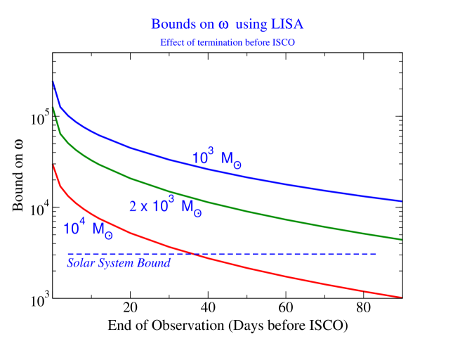
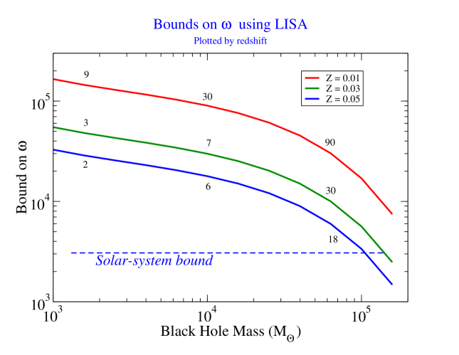
We first consider a NS in a quasi-circular inspiral into a BH of mass ranging from to and an integration time on LISA of one year leading up to the innermost stable orbit. We assume a SNR of 10. The parameter errors found are shown in Table I. For MBH masses less than about 70,000 , the bound on exceeds the current solar-system value of 3000, and for low mass black holes (), the bound could be 80 times larger. We then determine the bounds on for the same range of masses, and for orbits terminating at the ISCO, but for shorter integration times, such as 1/2 year or 1/4 year. The results are plotted in Fig. 1. Also shown in Fig. 1 are the approximate distances to which such systems can be observed. As expected, the bounds weaken almost in direct proportion to integration time. Figure 2 illustrates the effect of failing to observe the final orbits leading to the ISCO: shown for various BH masses are the bounds for one year of integration terminating a given number of days before the ISCO. The rapid fall-off of the bound with time before the ISCO indicates the importance of seeing the highest frequency, most relativistic orbits. For sources at a given redshift (corresponding to a given ), the SNR can be calculated from Eq. (31), and this used to determine the relevant bound on . The results for and are plotted in Fig. 3. To convert from to , we use the formula for a matter dominated, spatially flat cosmology with a value of the Hubble parameter . The signal-to-noise ratios for several illustrative cases are shown in the figure.
In principle, white-dwarf inspirals should give stronger bounds on because their sensitivities are much smaller than that of black holes. However, for small enough black hole mass, tidal disruption will require terminating the matched filter before the ISCO, with a consequent loss of accuracy in bounding , as indicated in Fig. 2. We take, as a crude measure of the termination of integration for a white dwarf inspiral, the Roche radius , where is the radius of the white dwarf, or equivalently, the place where the gravitational-wave frequency is given by . Using the approximation, for a non-relativistic WD equation of state, , and substituting into Eq. (29), we find an approximate cut-off time before the ISCO given by
| (32) |
When becomes negative (for , for a WD), the cut-off is the ISCO. Using the Fisher information matrix, we calculate the bounds on for one year of integration of white dwarf inspirals down to the appropriate cut-off time, with a SNR of 10. For , the bounds are 2.8 times better than for neutron stars of the same mass, as expected from the difference in sensitivities, but for , the improvement gradually decreases because of the loss of orbits near the ISCO. For a BH, the bound is only 14 percent better than the corresponding neutron-star bound.
B Follow-up Missions to LISA
Concepts for a future advanced space-based interferometer have been developed, based on the LISA project, which, for want of an official name, we will dub “SuperLISA”. The motivation for this mission is to detect gravitational waves with a peak sensitivity between the ranges of LISA and the ground-based detectors, say around Hz. Here, it is hoped, there will exist a window free of astrophysically generated sources of background gravitational waves, such as the white dwarf binaries that contribute to noise in LISA below Hz. With such a window, it is hoped that cosmological backgrounds of gravitational waves may be detectable.
A hypothetical noise curve for this advanced detector is given by with , where [21]
| (33) | |||||
| (34) | |||||
| (35) |
With this sensitivity, SuperLISA should be able to detect inspirals of intermediate mass systems () to cosmological distances with large SNR. Applying the method of the previous subsection to the noise curve of Eq. (35), we find that detection of these signals from NS-MBH inspirals may allow SuperLISA to place even more dramatic bounds on scalar-tensor theory than LISA.
We assume integration times of one year terminating at the ISCO and a neutron star sensitivity of , and consider sources at fixed redshifts of . The bounds obtainable from a NS inspiralling to black holes of a few hundreds of solar masses exceed tens of millions, and are dramatically better than the solar-system value for essentially all BH masses between and (Fig. 4). For sources at redshift and , the SNR is well above 10. The drop in the bound on for is caused by the fact that the initial frequency (one year before the ISCO) for such low-mass systems is already around Hz, where the instrument has its highest sensitivity; most of the data in these cases is being taken against a rapidly increasing background of instrumental noise (mostly caused by lack of time resolution related to the instrument’s arm lengths), hence the bound weakens.
IV Conclusions
We have found that future observations of inspirals of neutron stars into massive black holes by space-based laser interferometric detectors such as LISA may place significant bounds on the scalar-tensor coupling parameter . For inspirals into black holes as low as , the bound could be as large as 240,000 (for a SNR of 10), 80 times larger than current solar-system bounds. The bound achievable decreases with increasing black hole mass, for a given SNR. A follow-up space interferometer, with a sensitive band at intermediate frequencies between those of LISA and the ground based interferometers could produce bounds in the tens of millions.
The bound on is a strong function of the integration time. For integration times shorter than the canonical one year, decreases almost in direct proportion, and if the incoming wave is not integrated up to the last stable orbit, then the possible bound on drops off sharply. For neutron-star sensitivities smaller than 0.2, all quoted bounds increase by the factor ;
Two important issues have not been addressed.
The first is our restriction to quasi-circular orbits. This approximation is reasonable for stellar mass inspirals of compact objects in galaxies, which are expected to be detectable by ground-based interferometers. These are systems where gravitational radiation damping has had sufficient time to circularize any pre-existing, two-body eccentric orbit. However, in dense galactic nuclei or in dense globular clusters containing massive black holes, compact objects are expected to be injected into highly eccentric orbits via interactions with a cloud of objects surrounding the hole, and to suffer frequent perturbations by these bodies during apholion passage.
Eccentricity in and of itself should not have a strong effect on the bounds we have inferred. A preliminary estimate of the effect of small eccentricity on wave detection shows a small drop in SNR for an inspiral with a small eccentricity. For eccentricities of or less, the drop in SNR be four percent or less if a quasi-circular inspiral template is used to match against an eccentric waveform. For eccentricities of 0.2 to 0.3, the drop in SNR will increase to at least 10% and may be as large as 35% for some systems. This drop in SNR will be accompanied by a similar drop in detection rates and in the bounds on . This drop is not too large, however, and can be made even less by using an eccentric waveform template (with appropriate BD terms) to match the detected gravitational wave. On the other hand, frequent, essentially random perturbations of the orbit of the compact object by surrounding stars will make parameter estimation very difficult, even in general relativity. How important this effect will be, and whether there exist good data analysis techniques to handle it, is a subject of active investigation.
The second issue is event rate for inspirals into the intermediate mass black holes () that give the best bounds on . While enough is known and speculated about the rate of occurrence of or binary BHs in the centers of galaxies to make such systems promising sources for LISA, little to nothing is known about black holes of mass or less. Until some estimate can be made of how BH are distributed in the Universe, it will also be uncertain whether or not neutron stars can be expected to exist around these black holes, and how these neutron stars are expected to behave as they inspiral. Nevertheless, there has been recent speculation, based on numerical simulations, modeling and some observation, that runaway growth of intermediate mass black holes may occur in globular clusters or in young compact star clusters near AGNs [22, 23]. Another mechanism that has been discussed is the gravitational collapse of the first stars, assumed to be very massive objects [24].
It is worth pointing out that testing fundamental theory does not require the same event rate that a viable gravitational-wave astronomy does. A rare occurrence of a source with just the right characteristics can provide a strong test of scalar-tensor gravity. By comparison, while 35 years of pulsar astronomy boasts an average pulsar discovery rate of about 3 per month (for a total of over 1000 pulsars), it took only one, PSR 1913+16, to test the general relativistic quadrupole for gravitational radiation damping. Still, an estimate of the rate of compact body inspiral into intermediate mass black holes would be desirable, in order to evaluate how truly feasible such tests of scalar-tensor gravity using space interferometers might be.
Acknowledgments
We are grateful to Achamveedu Gopakumar, Matt Visser, and Sterl Phinney for useful discussions. This work is supported in part by the National Science Foundation Grant No. PHY 96-00049 and PHY 00-96522, and the National Aeronautics and Space Administration Grant No. NAG 5-10186.
REFERENCES
- [1] Email address for all correspondence: cmw@wuphys.wustl.edu
- [2] C. M. Will, Phys. Today 52, 38 (Oct.) (1999).
- [3] C. M. Will, Phys. Rev. D 50, 6058 (1994).
- [4] K. Danzmann, for the LISA Science Team, Class. Quantum Grav. 14, 1399 (1997).
- [5] C. Cutler, T. A. Apostolatos, L. Bildsten, L. S. Finn, É. E. Flanagan, D. Kennefick, D. M. Marković, A. Ori, E. Poisson, G. J. Sussman, and K. S. Thorne, Phys. Rev. Lett. 70, 2984 (1993) (gr-qc/9208005).
- [6] C. Brans, and R. H. Dicke, Phys. Rev. 124, 925 (1961).
- [7] C. M. Will, Living Reviews in Relativity 4, No. 4 (2001), avilable at http://www.livingreviews.org/Articles/Volume4/2001-4.
- [8] T. M. Eubanks, J. O. Martin, B. A. Archinal, F. J. Josties, S. A. Klioner, S. Shapiro, S. and I. I. Shapiro, preprint, available at ftp://casa.usno.navy.mil/navnet/postscript/prd_15.ps.
- [9] D. M. Eardley, Astrophys. J. Lett. 196, L59 (1975).
- [10] C. M. Will, Astrophys. J. 214, 826 (1977).
- [11] C. M. Will and H. W. Zaglauer, Astrophys. J. 346, 366 (1989).
- [12] T. Damour and G. Esposito-Farèse, Phys. Rev. D 54, 1474 (1996) (gr-qc/9602056); ibid. 58, 042001 (1998) (gr-qc/9803031).
- [13] H. W. Zaglauer, Astrophys. J. 393, 685 (1992).
- [14] The exception to this statement is a class of generalized scalar-tensor theories in which the scalar field exhibits an instability to “spontaneous scalarization” in the strong-field interiors of neutron stars, thereby enhancing the difference in sensitivities between even quite similar neutron stars, such as in the binary pulsar. For details, see [12].
- [15] L. S. Finn, Phys. Rev. D 46, 5236 (1992); L. S. Finn and D. F. Chernoff, ibid. 47, 2198 (1993) (gr-qc/9301003).
- [16] C. Cutler and É. Flanagan, Phys. Rev. D 49, 2658 (1994) (gr-qc/9402014).
- [17] E. Poisson and C. M. Will, Phys. Rev. D 52, 848 (1995) (gr-qc/9502040).
- [18] C. M. Will, Phys. Rev. D 57, 2061 (1998) (gr-qc/9709011).
- [19] P. Bender, I. Ciufolini, K. Danzmann, W. Folkner, J. Hough, D. Robertson, A. Rüdiger, M. Sandford, R. Schilling, B. Schutz, R. Stebbins, T. Summer, P. Touboul, S. Vitale, H. Ward, and W. Winkler, LISA: Laser Interferometer Space Antenna for the Detection and Observation of Gravitational Waves, Pre-Phase A Report, December 1995 (unpublished).
- [20] P. L. Bender and D. Hils, Class. Quantum Grav. 14, 1439 (1997).
- [21] K. S. Thorne, private communication.
- [22] M. C. Miller and D. P. Hamilton, submitted to Mon. Not. Roy. Astron. Soc. (astro-ph/0106188).
- [23] T. Ebisuzaki, J. Makino, T. G. Tsuru, Y. Funato, S. Portegies Zwart, P. Hut, S. McMillan, S. Matsushita, H. Matsumoto and R. Kawabe, submitted to Astrophys. J. Lett. (astro-ph/0106252).
- [24] R. Schneider, A. Ferrara, B. Ciardi, V. Ferrari and S. Matarrese, Mon. Not. Roy. Astron. Soc. 317, 385 (2000) (astro-ph/9909419).

| Bound | ||||||||
|---|---|---|---|---|---|---|---|---|
| (s) | (%) | (%) | on | |||||
| 1000 | 2.39 | 12.3 | .000192 | .0727 | 244549 | .885 | -.996 | -.919 |
| 5000 | 3.80 | 11.7 | .000544 | .0252 | 56326 | .970 | -.998 | -.953 |
| 10000 | 5.32 | 12.9 | .000768 | .0180 | 29906 | .978 | -.997 | -.961 |
| 50000 | 26.54 | 32.0 | .00243 | .0145 | 4780 | .989 | -.998 | -.978 |
| 100000 | 103.07 | 84.8 | .00610 | .0219 | 1458 | .993 | -.999 | -.986 |