A numerical testbed for singularity excision in moving black hole spacetimes

Abstract

We evolve a scalar field in a fixed Kerr-Schild background geometry to test simple $(3+1)$-dimensional algorithms for singularity excision. We compare both centered and upwind schemes for handling the shift (advection) terms, as well as different approaches for implementing the excision boundary conditions, for both static and boosted black holes. By first determining the scalar field evolution in a static frame with a $(1+1)$-dimensional code, we obtain the solution to very high precision. This solution then provides a useful testbed for simulations in full $(3+1)$ dimensions. We show that some algorithms which are stable for non-boosted black holes become unstable when the boost velocity becomes high.

]

I Introduction

The long-term numerical evolution of black holes is one of the most important and challenging problems in numerical relativity. Simultaneously, it is a problem for which a solution is very urgently needed; binary black holes are among the most promising sources for the gravitational wave laser interferometers currently under development, including LIGO, VIRGO, GEO, TAMA and LISA, and theoretically predicted gravitational wave templates are crucial for the identification and interpretation of possible signals.

Numerical difficulties arise from the complexity of Einstein’s equations and the existence of a singularity inside the black hole (BH). Numerical simulations based on the traditional Arnowitt-Deser-Misner (ADM) decomposition in $(3+1)$ dimensions, for example, often develop instabilities [1, 2]. The gauge (coordinate) freedom inherent to general relativity constitutes a further complication. Singularity avoiding slicings [3, 4, 5] can follow evolutions involving black holes only for a limited time, since the stretching of time slices typically causes simulations to crash on time scales far shorter than the time required for a binary BH orbital period.

Recently, there have been several very promising numerical breakthroughs. Stable formulations of Einstein’s equations using a conformal-tracefree decomposition have been developed by Shibata and Nakamura [6] and by Baumgarte and Shapiro [2]. The so-called BSSN formulation has shown remarkable stability properties when compared to the ADM formulation in a wide range of numerical simulations [7, 8, 9, 10, 11, 12]. Also, the development of “singularity excision” techniques [13, 14, 15, 16, 17], excising the singularity from the computational domain, may allow for long term binary BH evolutions (see [18] for preliminary results). There have also been proposals [19, 20, 21] for alternative families of binary initial data based on the Kerr-Schild form of the Schwarzschild (or Kerr) metric to represent each of the BHs. The use of Kerr-Schild coordinates is desirable for the numerical evolution of BHs and suitable for applying singularity excision techniques because the coordinates smoothly penetrate the horizon of the holes. Moreover, they provide a natural framework for constructing initial data without assuming conformal flatness, essential for representing non-distorted Kerr Black holes.

Typically, the numerical grid extends into the black hole in singularity excision applications. Moreover, the shift vector sometimes becomes larger than unity, so that some finite difference stencils become “acausal” and therefore unstable. To avoid this problem, “causal differencing” [14, 16] or “causal reconnection” schemes [22] have been suggested (see also [17, 23, 24, 25, 26, 27, 28]). Unfortunately, these schemes are fairly involved and complicated.

Alcubierre et al [29, 30] recently proposed a simple BH excision algorithm for a non-boosted distorted BH evolution which avoids the complications of causal differencing. Their algorithm is based on the following simplifications: (a) excise a region adapted to Cartesian coordinates, (b) use a simple inner boundary condition at the boundary of the excision zone, (c) use centered differences in all terms except the advection terms on the shift, where upwind differencing along the shift direction is used. Their algorithm is quite successful and allows for accurate and stable evolution of non-boosted distorted BHs for hundreds of dynamical times.

Here we devise an experiment to test some simple singularity excision algorithms for evolving dynamical fields in numerical 3D black hole spacetimes. Our goal is to identify a numerical scheme which is simple and stable like the one presented in [29] for non-boosted BHs but can also handle moving BHs. Our experiment consists of tracking the propagation of a scalar field in the fixed background spacetime of a Kerr-Schild BH. By first solving for the evolution in a static frame by means of a 1D code, we obtain the solution to arbitrary accuracy. We then perform simulations in full 3D for both stationary and boosted Kerr-Schild BHs, using our 1D “exact” results for detailed comparison. We use this testbed to compare schemes which handle advection terms by centered versus upwind differencing. We also run our experiment for different implementations of the excision boundary conditions. Our aim is to find numerical stencils which we can later adapt to a BSSN scheme for evolving dynamical spacetimes with moving (e.g., binary) BHs. While the proving ground we construct here employs a fixed background geometry, we feel that it furnishes necessary, if not sufficient, conditions that must be met for a field evolution scheme in any numerical spacetime containing BHs. We provide this report to convey the utility of this testbed as a quick diagnostic of alternate differencing stencils and with the hope that it might prove helpful for other 3D code builders.

Our results show that, in general, an upwind scheme is more stable than a centered scheme. This is consistent with the results of [29]. We also find that a higher resolution is needed for an upwind than for a centered scheme to achieve a desired accuracy, due to the diffusive character of an upwind scheme. We find that the numerical implementation used in [29] is stable in the non-boosted case but unstable in the boosted case. However, the stability can be restored by using an alternative excision boundary condition which is stable in both the non-boosted and boosted cases. In all the cases studied, the use of a third-order extrapolation condition at the excision boundary is required for stable runs.

The paper is organized as follows: We describe the Kerr-Schild BH spacetime and the scalar field equation in this background geometry in Sec. II. Sec. III is devoted to a discussion of initial data, numerical algorithms, and different boundary conditions. We present our 3D numerical results, and compare them to very accurate 1D results in Sec. IV. We summarize and discuss the implications of our findings in Sec. V. We also include two Appendices. Appendix A sketches the von Neumann stability analysis of the 1D centered and upwind schemes. Appendix B describes the Lorentz transformation of a scalar wave. Throughout the paper we adopt geometrized units with $G=c=1$.

II Basic equations

A Kerr-Schild form of the Schwarzschild spacetime

The ingoing Kerr-Schild form of the Kerr metric is given by

$$ds^{2}=(\eta_{\mu\nu}+2H\ell_{\mu}\ell_{\nu})dx^{\mu}dx^{\nu},$$ (1)

(see [19, 31]), where $\mu$, $\nu$ run from $0$ to $3$, $\eta_{\mu\nu}={\rm diag}(-1,1,1,1)$ is the Minkowski metric in Cartesian coordinates, $H$ is a scalar function. The vector $\ell_{\mu}$ is null both with respect to $\eta_{\mu\nu}$ and $g_{\mu\nu}$,

$$\eta^{\mu\nu}\ell_{\mu}\ell_{\nu}=g^{\mu\nu}\ell_{\mu}\ell_{\nu}=0,$$ (2)

and we have $\ell^{2}_{t}=\ell^{i}\ell_{i}$. The spacelike hypersurfaces extend smoothly through the horizon, and gradients near the horizon are well-behaved. Comparing the metric (1) with the “ADM” metric typically used in $3+1$ formulations, one identifies the lapse function $\alpha$, shift vector $\beta_{i}$ and the spatial 3-metric ${}^{(3)}g_{ij}$ as

$$\begin{array}[]{rcl}\alpha&=&1/\sqrt{1+2H\ell^{2}_{t}},\\ \beta_{i}&=&2H\ell_{t}\ell_{i},\\ {}^{(3)}g_{ij}&=&\eta_{ij}+2H\ell_{i}\ell_{j}.\end{array}$$ (3)

For the time-independent Schwarzschild spacetime (the “Eddington-Finkelstein form” [32]) in Cartesian coordinates we have

$$\begin{array}[]{rcl}H&=&M/r,\\ \ell_{\mu}&=&(1,x_{i}/r),\end{array}$$ (4)

where $M$ is the total mass-energy and $r^{2}=(x^{1})^{2}+(x^{2})^{2}+(x^{3})^{2}$. The Kerr-Schild metric (1) is form-invariant under Lorentz transformations. Applying a constant Lorentz transformation $\Lambda$ (with boost velocity ${\bf v}$ as specified in the background Minkowski spacetime) to (1) preserves the Kerr-Schild form, but with transformed values for $H$ and $\ell_{\mu}$ (see [19])

$$\begin{array}[]{rcl}x^{\prime\alpha}&=&\Lambda^{\alpha}{}_{\beta}x^{\beta},\\ H(x^{\alpha})&\rightarrow&H(\Lambda^{-1\alpha}{}_{\beta}x^{\prime\beta}),\\ \ell_{\mu}^{\prime}&=&\Lambda^{\nu}{}_{\mu}\ell_{\nu}(\Lambda^{-1\alpha}{}_{\beta}x^{\prime\beta}),\\ g_{\mu\nu}^{\prime}&=&\eta_{\mu\nu}+2H\ell_{\mu}^{\prime}\ell_{\nu}^{\prime},\end{array}$$ (5)

Now let $x^{\alpha}$ and $x^{\prime\beta}$ be the coordinates in the lab frame $X$ and the comoving (with the BH) frame $X^{\prime}$. For the Eddington-Finkelstein system boosted in the $xy$-plane ($v_{3}=0$), in the lab frame $X$ we have

$$r^{2} = \gamma^{2}(v_{1}\overline{x}+v_{2}\overline{y})^{2}+\overline{x}^{2}+\overline{y}^{2}+z^{2},$$ (6)

$$\ell_{t} = \gamma[1-\gamma(v_{1}\overline{x}+v_{2}\overline{y})/r],$$ (7)

$$\ell_{x} = \overline{x}/r-v_{1}\ell_{t},$$ (8)

$$\ell_{y} = \overline{y}/r-v_{2}\ell_{t},$$ (9)

$$\ell_{z} = z/r,$$ (10)

where $\gamma=1/\sqrt{1-v^{2}}$ and $v^{2}=v_{1}^{2}+v_{2}^{2}$. $\overline{x}$ and $\overline{y}$ are defined as $\overline{x}\equiv x-v_{1}t$ and $\overline{y}\equiv y-v_{2}t$. Under a boost the metric becomes explicitly time dependent. Since the boost of the Schwarzschild solution merely “tilts the time axis”, we can consider all the boosted $3+1$ properties at an instant $t=0$, in the frame which sees the hole moving. Subsequent time $t$ simply offset the solution by an amount $vt$. With Eqs. (8) $\alpha$ and $\beta_{i}$ are defined via Eq. (3).

B The scalar field equation

The field equation for a massless scalar field is

$$\Box\phi=0,$$ (11)

which can be expanded as

$$g^{\mu\nu}\phi_{;\mu;\nu}={1\over\sqrt{-g}}(\sqrt{-g}g^{\mu\nu}\phi_{,\mu})_{,\nu}=0.$$ (12)

We can decompose this second-order equation into two first-order-in-time equations by defining the auxiliary variable $\pi\equiv\Phi_{,t}-\beta^{i}\Phi_{,i}$, where $\Phi\equiv r\phi$, obtaining,

$$\left\{\begin{array}[]{rcl}\Phi_{,t}&=&\beta^{i}\Phi_{,i}+\pi,\\ \pi_{,t}&=&\beta^{i}\pi_{,i}+{\cal F}.\end{array}\right.$$ (13)

Here

$${\cal F} = -{1\over g^{00}}\left({}^{(3)}g^{ij}\Phi_{,i,j}+A^{i}\Phi_{,i}+B\pi+{C\over r^{2}}\Phi\right),$$ (14)

$$A^{i} = g^{i\mu}{}_{,\mu}-{2\over r}g^{i\mu}(\ell_{\mu}+V_{\mu})+g^{0\mu}\beta^{i}{}_{,\mu}+B\beta^{i},$$ (15)

$$B = g^{0\mu}{}_{,\mu}-{2\over r}g^{0\mu}(\ell_{\mu}+V_{\mu}),$$ (16)

$$C = g^{\mu\nu}\left(3(\ell_{\mu}+V_{\mu})(\ell_{\nu}+V_{\nu})-\eta_{\mu\nu}-V_{\mu}V_{\nu}\right)$$ (18)

$$-rg^{\mu\nu}{}_{,\nu}(\ell_{\mu}+V_{\mu}),$$

$$g^{0\mu}\beta^{i}{}_{,\mu} = {\beta^{i}\over r}\left(\alpha^{2}(3\ell_{t}-2\gamma)-2\gamma-3\beta^{i}V_{i}+{1\over\ell_{t}}\right)$$ (20)

$$+{V^{i}\over r}(1-\alpha^{2}),$$

and $V_{\mu}\equiv\gamma(-1,v_{i})$ is the 4-vector of the velocity ${\bf v}$ in Cartesian coordinates.

In the comoving (non-boosted) frame, the scalar field equation (11) can be cast into a 1D radial equation which, for spherical waves, reduces to

$$\left(-(1+2H)\partial^{2}_{t^{\prime}}+4H\partial_{t^{\prime}}\partial_{r^{\prime}}+(1-2H)\partial^{2}_{r^{\prime}}-{2\over{r^{\prime}}}H\partial_{t^{\prime}}\right.$$ (21)

$$\qquad\left.+{2\over r^{\prime}}H\partial_{r^{\prime}}-{2H\over{r^{\prime}}^{2}}\right)\Phi=0.$$ (22)

Eq. (22) can again be decomposed into two first-order-in-time equations

$$\left\{\begin{array}[]{rcl}\Phi_{,t^{\prime}}&=&\beta^{r^{\prime}}\Phi_{,r^{\prime}}+\pi,\\ \pi_{,t^{\prime}}&=&\beta^{r^{\prime}}\pi_{,r^{\prime}}+f,\end{array}\right.$$ (23)

where

$$f = {1\over(1+2H)^{2}}\partial^{2}_{r^{\prime}}\Phi+{2H\over r^{\prime}(1+2H)^{3}}\partial_{r^{\prime}}\Phi$$ (25)

$$-{2H\over r^{\prime}(1+2H)}\pi-{2H\over r^{\prime 2}(1+2H)}\Phi,$$

$$\beta^{r^{\prime}} = {2H\over 1+2H}.$$ (26)

The characteristics (which can be derived from metric Eq. (1)) of the scalar field Eq. (23) have speeds $-1$ and $(r^{\prime}-2M)/(r^{\prime}+2M)$.

In the following sections we solve Eq. (13) with a 3D code and Eq. (23) with a 1D code and compare the results. Since the 1D code can be used with almost arbitrary resolution, we can effectively compare our 3D results with an “exact” numerical solution.

III Initial data, Numerical algorithms and boundary conditions

A Initial value

As initial data for the scalar field in the comoving frame of the BH, we choose a spherical Gaussian of width $\sigma$ centered at radius $r_{0}^{\prime}$

$$\Phi(0,x^{\prime},y^{\prime},z^{\prime})=\exp\left(-{(r_{*}^{\prime}(r^{\prime})-r_{*}^{\prime}(r_{0}^{\prime}))^{2}\over\sigma^{2}}\right)$$ (27)

where $r_{*}^{\prime}\equiv r^{\prime}+2M\ln(r^{\prime}/2M-1)$ is the tortoise coordinate (compare [33]). For all calculations in this paper we choose $r_{0}^{\prime}=10M$ and $\sigma=1M$. According to (27) $\Phi$ vanishes on the event horizon. We also assume time symmetry at $t=0$

$$\partial_{t}\Phi(0,x^{\prime},y^{\prime},z^{\prime})=0.$$ (28)

so that

$$\pi(0,x^{\prime},y^{\prime},z^{\prime})=-\beta^{i^{\prime}}\partial_{i^{\prime}}\Phi(0,x^{\prime},y^{\prime},z^{\prime}).$$ (29)

As the wave packet evolves in time, it splits, with one part of it propagating outwards towards null infinity and the other propagating inwards towards the horizon. Near the horizon, the wave undergoes partial transmission and reflection. We calculate the waveform of the scattered scalar wave as observed at some fixed distance from the BH and compare the 3D results with the “exact” 1D waveform.

FIG. 1.: The initial data in the lab frame $X$ and in the comoving frame $X^{\prime}$. The bold solid line segments represent the wave packets (initial data) in different frames, the dashed lines indicate the propagations of the wave packets in spacetime. The initial data in $X$ (at $t=0$) can be obtained by the future and past evolution of the scalar field with the initial data in $X^{\prime}$ (at $t^{\prime}=0$).

For the boosted cases, the initial data is different from the non-boosted case due to the tilt of axes (see Fig. 1). The frame $X^{\prime}(t^{\prime},{\bf x}^{\prime})$ (comoving with the BH) moves along $x$-axis with a boost velocity relative to the lab frame $X(t,{\bf x})$. The initial data in $X$ can be derived by evolving the scalar field in $X^{\prime}$, followed by a Lorentz transformation. (Refer to Appendix B for details.)

B Differencing scheme

recipe	advection term	advection term	inner		stable?
	outside BH	inside BH	boundary	$v=0$	$v=0.2$	$v=0.5$
AI	C	C	E	Yes	Yes	No
AII	C	U	E	Yes	Yes	Yes
BI	U	U	P	Yes	No	No
BII	U	U	E	Yes	Yes	Yes

TABLE I.: Summary of recipes AI, AII, BI, and BII, and their stability properties for the three different boosts. The boldface letters denote C: centered scheme; U: upwind scheme ; E: third-order extrapolation condition; P: copying the time derivative of every field at the boundary from the interpolated value just outside the excision zone along the normal direction. We analyzed the stability of these recipes for static black holes ($v=0$) and boosts with speed $v=0.2$ and $v=0.5$. Recipe BI, which is based on the implementation of [29] passes the non-boosted case but fails in the boosted cases. Recipe AI passes the non-boosted case and the $v=0.2$ boosted case but fails in the $v=0.5$ case. Recipe AII and BII pass all tests that we have performed.

FIG. 2.: Schematic diagram of shift advection stencils in the computational domain and around an excision zone. The dashed circles inside the excision zone are the grid points to which the extrapolated values are assigned by using Eq. (34).

We are looking for simple and robust recipes and focus, as in [29], on the shift terms in the field equation, which we regard as a generic “advection” terms (terms that look like $\beta^{i}\partial_{i}$). We apply both centered and upwind schemes to these advection terms to test their stability. All other derivative terms are evaluated using centered differencing.

Consider the gridpoint with array indices $i$, $j$, and $k$ in the $x$, $y$, and $z$ directions, respectively. With centered differencing, the first derivative of $\Phi$ with respect to $x$ at this gridpoint is

$$(\Phi_{,x})_{i,j,k}={1\over 2\Delta x}[\Phi_{i+1,j,k}-\Phi_{i-1,j,k}].$$ (30)

For the upwind scheme the second-order accurate first derivative along $x$-direction is

$$(\Phi_{,x})_{i,j,k} = -{\nu_{1}\over 2\Delta x}[\Phi_{i+2\nu_{1},j,k}$$ (32)

$$\qquad\qquad-4\Phi_{i+\nu_{1},j,k}+3\Phi_{i,j,k}],$$

where $\nu_{1}$ is defined as

$$\nu_{1}\equiv{\beta^{1}\over|\beta^{1}|}=\left\{\begin{array}[]{ll}1&\mbox{for}\quad\beta^{1}>0,\\ -1&\mbox{for}\quad\beta^{1}<0.\end{array}\right.$$ (33)

We use analogous differencing in the $y$- and $z$-directions (see Fig. 2).

Different schemes can be used inside/outside the event horizon in each recipe to further isolate where and how any instability arises. In this paper, we consider $4$ different recipes which we call AI, AII, BI, and BII (see Table I). Recipes AI, AII, and BII all use the extrapolation inner boundary condition (see Sec. III D below). In recipe AI, the centered scheme is used for finite differencing on the shift advection term everywhere. This scheme is stable according to a van-Neumann stability analysis since $\beta^{i}$ is never greater than unity in the Kerr-Schild metric (refer to Appendix A for a stability analysis). In AII, the upwind scheme is used inside the BH and the centered scheme is used outside the BH for the shift term. In BII, upwind differencing is used everywhere.

Recipe BI, which is based on the implementation of [29], differs from the other schemes in its excision boundary condition. Alcubierre and Brügmann [29] use a cubic excision zone and copy the time derivative of every field at a gridpoint just inside the excision zone from the neighboring gridpoint just outside. Our excision zone is spherical with radius $r^{\prime}=M$ (in the comoving frame). To generalize the scheme of [29] we interpolate neighboring gridpoints to the normal on the surface of the excised region. More specifically, for a gridpoint $(i,j,k)$ just inside the excised region we take its nearest neighbors along the coordinate axes away from the center of the black hole, say $(i+1,j,k)$, $(i,j+1,k)$ and $(i,j,k+1)$. These three points define a plane, and we interpolate to the intersection of this plane with the normal on the surface of the excised region. If one of these three neighbors is still in the excised region, we project the normal into the plane spanned by the remaining two coordinate axes, and do the interpolation there; if two of the neighbors are inside the excised region we directly copy the remaining third point. If all three points are inside the excised region we repeat the procedure with the three points $(i+1,j+1,k)$, $(i+1,j,k+1)$ and $(i,j+1,k+1)$; if that is also not successful we finally copy the point $(i+1,j+1,k+1)$. This particular algorithm is only one of many possibilities. We have experimented with a number of other schemes, and have found that the stability properties do not depend on the details of this implementation. Like BII, BI also uses the upwind scheme to compute the shift advection terms everywhere.

C Outer boundary conditions

At the outer boundary, we impose an outgoing wave boundary condition. In this approximation, we assume that the functions are of the form $\Phi=f(\lambda t-R)$ (since $\Phi=r\phi$), where $\lambda=(R-2M)/(R+2M)$ is the outgoing characteristic speed. The values $f(t+\Delta t,R)$ of the grid points at the outer boundary are updated by using the value $f(t,R-\lambda\Delta t)$ with second-order interpolation. In the boosted cases, the characteristics $\lambda$ at the outer boundary are derived from the relativistic addition of the characteristic in the comoving frame and the boost velocity.

This boundary condition provides a stable outer boundary provided that the outer boundary is placed at a sufficiently large distance. With the outer boundary at finite radii, as in our cases, some reflected waves are created at the boundary. (We find that reflection waves with larger amplitude will appear if the true characteristic speed $\lambda$ in $f$ is replaced by $1$) The amplitude of the reflected wave decreases as resolution is increased. In boosted cases, the effect of the inaccurate outer boundary condition cannot be ignored as the BH approaches the outer boundary. For our tests, however, the reflected waves from the boundary are small perturbations of the field and do not affect the stability of different recipes, only the accuracy.

D Inner boundary conditions

At the inner boundary we use a singularity excising method (see, e.g. [14, 16, 17, 24, 34, 35, 36]). In general dynamic spacetimes, the location of the apparent horizon is not known a priori, and must be computed at each time step with an “apparent horizon finder” (e.g. [37, 38, 39]). This is not the case for the present static Schwarzschild background since the location of the apparent (and event) horizon is known at all times [40]. On the other hand, it is not necessary to know the exact location of the apparent horizon to implement the singularity-excising method, provided the excision zone is sufficiently small that one can be confident that it lies entirely inside the horizon. We choose to excise the region with radius $r^{\prime}=1M$ from the center of BH where $r^{\prime}$ is the radial distance measured in the comoving frame $X^{\prime}$. The simplest inner boundary condition obtains, by extrapolation, the field variables at gridpoints just inside the masked region from gridpoints just outside this region. These values can then be used in a centered evolution scheme to update the field variables at gridpoints just outside the excision zone. We have implemented such a boundary condition using a third-order extrapolation scheme

$$f_{j-\nu}=4f_{j}-6f_{j+\nu}+4f_{j+2\nu}-f_{j+3\nu},$$ (34)

in all recipes except BI. Here $j$ is a gridpoint just outside the excised region, and, with $\nu$ either $+1$ or $-1$, $j-\nu$ is just inside (see Fig. 2). We apply this algorithm along whichever axis the second derivative is taken, for example along the $x$-axis for a second derivative with respect to $x$. With this extrapolation, the second spatial derivatives using centered differencing are second-order accurate. This is equivalent to using a second-order one-sided differencing scheme. These boundary conditions do not violate causality since no information is extracted from within the excision zone. This prescription is simple to implement and does not require special assumptions on the behavior of the variables in the proximity of the excision zone. A similar implementation has proven to be stable for wave propagation in $2+1$ dimensions on a flat spacetime [35].

In recipe BI, we generalize the implementation of [29] and copy the time derivative of every field variable at the boundary from interpolated values just outside the excised region as described in Sec. III B. As we will show in Sec. IV, this inner boundary condition will produce stable results in the non-boosted BH case, but results in an instability when the BH moves and grid points emerging from the excision zone must be assigned by extrapolation.

E Extrapolation to newly emerging grid points

FIG. 3.: Convergence tests for our 1D evolution calculations, using recipe AI (left panel) and BII (right panel). To demonstrate second order convergence, we plot the appropriately rescaled finite difference error ${\rm Err}_{\Delta r}=\Phi_{\Delta r/2}-\Phi_{\Delta r}$ at the check point $r=14M$ for various resolutions $\Delta r$.

We use a second-order extrapolation scheme to set values at gridpoints that are newly emerging from the excision zone as the BH travels through the numerical grid. If available, we carry out the extrapolation along the $z$-axis, because the BH is boosted in the $xy$-plane, and the extrapolated values along the $z$-direction are least affected by numerical errors from previous extrapolations in the evolution. If the points needed for this extrapolation are themselves excised, we instead average between extrapolations along the $x$ and $y$ directions or use only one of the two if the other one is not available (because the necessary points are excised). If neither one is available we continue through the following hierarchy of preferred extrapolation directions: $z$, then $x$ and $y$, then $xz$ and $yz$, finally the $xy$- and $xyz$-directions. We have experimented with other extrapolation prescriptions and have found that the stability properties of the code are fairly insensitive to the details of this scheme.

IV numerical results

FIG. 4.: The scalar field $\Phi$ as a function of $t$ at radius $r=14M$ in the non-boosted 3D case. In each panel, the solid curve is the 1D solution, while the dotted, dashed and dot-dashed line are 3D solutions computed for grid widths $\Delta=0.125M$, $\Delta=0.25M$, and $\Delta=0.5M$, respectively. We also include convergence tests for each recipe in the insets, where the dotted line is $16\times{\rm Err}_{0.125M}$, the dashed line is $4\times{\rm Err}_{0.25M}$, and the dot-dashed line is ${\rm Err}_{0.25M}$. Here the finite difference error is computed from ${\rm Err}_{\Delta x}\equiv\Phi_{\Delta x}-\Phi_{\rm 1d}$.

We numerically solve both the 1D and 3D scalar wave equations (13) Eq. (23) using an iterative Crank-Nicholson scheme with two corrector steps [41]. Since the 1D code can be run with an essentially arbitrary number of radial grid points and hence essentially arbitrary accuracy, we use this solution as the “exact” solution for comparisons.

We compare the results from the 3D simulations using the four recipes (see Table. I) for both the non-boosted and boosted cases. There are two sub cases of the boosted case: a “slow” boost speed $v=0.2$ and a “fast” boost speed $v=0.5$. The results for both boosted cases are summarized in Table. I, but we will discuss in detail only the $v=0.5$ boost case.

In each case, we compare the waveforms with the 1D result for three uniform grid resolutions $\Delta=0.5M$, $\Delta=0.25M$,and $\Delta=0.125M$. We choose a time step $\Delta t=\Delta/4$ in all cases, and assume equatorial symmetry across the $z=0$ plane.

In the non-boosted case, the computational domain is $32M\times 32M\times 16M$ ($-16M<x<16M$,$-16M<y<16M$,$0<z<16M$). In the $v=0.5$ case, the domain is extended to $48M\times 48M\times 24M$ ($-20M<x<28M$,$-24M<y<24M$,$0<z<24M$). A larger spatial domain is needed in the high speed case to observe the BH’s motion before it moves out of the computational domain. In each 3D case the code with $\Delta=0.125M$ resolution is run only to $t=10M$ to check its stability and convergence; the lower resolution non-boosted cases are run until $t=100M$, and the lower resolution boosted cases are run until $t=48M$.

A 1D result

We verify the second-order accuracy of our 1D codes in Fig. 3. We compare the amplitude difference between the results observed from the check point $r=14M$ by continual doubling of the grid resolution. We present results for recipe AI in the left panel of Fig. 3 and for BII in the right panel. Comparing the scales of ${\rm Err}_{\Delta r}$ in the two panels shows that, while both scheme are second order accurate, the centered scheme of recipe AI converges much faster than the more diffusive upwind scheme of recipe BII. We find very similar results in the 3D codes below.

B 3D results in co-moving coordinates

FIG. 5.: The scalar field $\Phi$ as a function of time for a boost with $v=0.5$ for checkpoints at ($14M$,$0$,$0$), ($0$,$14M$,$0$), and ($-14M$,$0$,$0$) (from left to right). The inset in each panel is the blowup of the waveform for early times. The first and second rows are the results for recipes AII and BII respectively. In each panel, the solid curve is the 1D solution, while the dotted, dashed and dot-dashed line are 3D solutions for grid resolutions $\Delta=0.125M$, $\Delta=0.25M$, and $\Delta=0.5M$. In the third column, for checkpoint ($-14M$,$0$,$0$), we only show the two coarser resolutions.

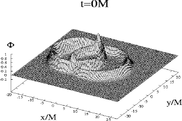
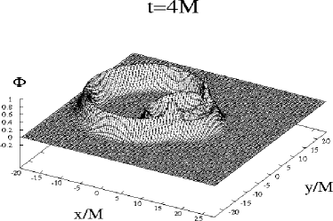
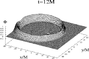
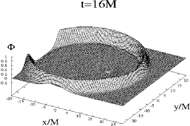
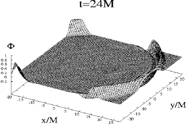
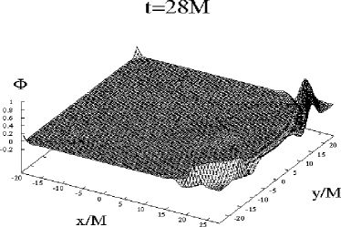
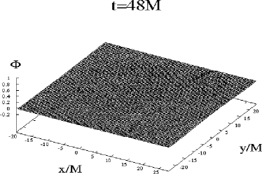
FIG. 6.: The snapshots of the scalar field as evolved by recipe BII in the boosted $v=0.5$ case ($z=0.125M$).

We first study the four recipes AI, AII, BI and BII for the non-boosted (comoving) case. All four recipes give stable results and converge to the 1D result, as shown in Fig. 4. The stability of recipe BI is consistent with the conclusion of [29] in which the recipe gives a stable and accurate solution in a non-boosted distorted BH.

In Fig. 4 the first peak and the first minimum in the waveform curves are produced by the part of the wave packet which moves outwards and leaves the computational grid. The minimum observed at $t\approx 10M$ is a numerical artifact and converges away for increasing grid resolution. We demonstrate the second order convergence of the algorithms in the insets in Fig. 4. For the upwind schemes of recipes BI and BII the convergence is much slower than for the centered schemes of recipes AI and AII, as expected from the 1D results (see Fig. 3). There are several bumps at $t\approx 10M$, $t\approx 30M$, and $t\approx 50M$. These are the reflection waves coming from the outer boundaries due to the approximate outer boundary condition. We find that these bumps can always be diminished significantly by extending the outer boundary to a larger radius and/or increasing the resolution.

The waveforms in Fig. 4 also show that the upwind scheme (recipes BI & BII) efficiently eliminates high frequency noise. This property is very helpful in keeping the code stable, but the solution with low resolution can be very inaccurate. Therefore, higher resolution and, thus, greater computing resources are needed (compared to the centered scheme) to achieve a desired accuracy.

C 3D results in boosted frames

We now describe the boosted case with the boost speed $v=0.5$. In this case the BH, initially located in the origin of the lab frame, is boosted along the $x$-axis with the boost velocity ${\bf v}=(0.5,0,0)$. We stop the evolution when the separation between the center of BH and the boundary is less than $4M$ to avoid the BH being too close to the boundary. Since the origin of the lab frame is set such that the positive boundary of $x$-axis is at $x=28M$, the total evolution time is $24M/0.5=48M$.

Fig. 5 shows the waveforms of the scalar field. The boosted 1D results are derived from the non-boosted (comoving) 1D result with a Lorentz transformation (see Appendix B). We observe the scalar waveforms at three check points, located at ($14M$,$0$,$0$), ($0$,$14M$,$0$), and ($-14M$,$0$,$0$). In the first column of Fig. 5, there are two peaks in each waveform observed at ($14M$,$0$,$0$). The first peak is the incoming wave packet, and the second peak is the outgoing wave packet. This is more obvious in the 2D snapshots in Fig. 6 (see also Fig. 1). The waveforms are masked at $t=26.3M-29.7M$ in the first column of Fig. 5 because the excision zone passes over the check point during that time. The waveforms in the first column have larger amplitude changes from low resolution to high resolution. The situation is especially obvious for recipe BII (using the upwind scheme) in which the peak of $\Phi$ varies from $0.32$ at low resolution to $0.55$ at high resolution. We restricted the high resolution run to a computational domain ($-8M<x<24M$,$-16M<y<16M$,$0<z<16M$) in order to save computational resources. Accordingly, no high resolution results are available for the check point $(-14M,0,0)$. Fig. 5 shows that the 3D results of AII and BII still converge to the 1D solution although the rate of convergence for both recipes is somewhat worse than in the non-boosted case.

Recipe BI produces an instability for boosted BHs. We believe that this instability arises as a result of combining the simple inner boundary condition of recipe BI with the treatment of gridpoints that newly emerge from inside the excision zone. The error expands outward as the BH moves. Physically, nothing can emerge from the BH, but numerically noise can propagate outward through the event horizon. Since the third-order extrapolation (34) condition is equivalent to using a one-sided scheme at the excision boundary, it propagates any numerical errors inwards. We believe that this extrapolation produces the improved behavior seen in recipe BII. Furthermore, Eq. (34) is viable in all cases (non-boosted and boosted) as long as the excision zone is inside the event horizon.

AI is stable in the $v=0.2$ case but produces instability in $v=0.5$ case. We believe that this instability is again caused by the treatment of the grid points emerging from inside the excision zone, where numerical errors are allowed to propagate outwards by the centered scheme. The instability can be avoided by using the upwind scheme, which propagate the numerical errors inwards (e.g., recipe AII).

Recipe BII is stable in all the cases. Fig. 6 shows the stable evolution of the scalar field with recipe BII. The excision zone can be seen in the snapshots at $t=12M$, $t=16M$ and $t=24M$ where the residual wave amplitude is seen to hover about the excision zones centered at ($x$,$y$)$=$($6M$,$0$), ($8M$,$0$), and ($12M$,$0$) before disappearing entirely at later time inside the masked region. Recipe AII is also stable in all the cases, although the numerical errors in AII are bigger than in BII. We have also confirmed that recipes AII and BII are stable for boosts in off-axis directions by studying a boost of $v=0.5$ in the ${\bf v}=(0.4,0.3,0)$ direction.

V conclusion

We have compared four different numerical recipes for numerically evolving a scalar field in a Kerr-Schild BH spacetime. We have integrated the equations both in comoving and lab frames. We study the stability and convergence with the goal of identifying simple promising techniques for more general evolution problems. We used singularity excision and have experimented with the boundary conditions for the excision zone.

Our results show that, in general, an upwind scheme is superior to a centered scheme for maintaining stability. This is consistent with the results of [29]. We find that higher resolution is needed for an upwind scheme than for a centered one to achieve a desired accuracy due to the diffusive character of an upwind scheme.

As summarized in Table I, two of the four recipes are stable in all testbed scenarios: recipe AII, in which the upwind scheme is used on the shift (advection) term only inside the event horizon, and recipe BII, in which the upwind scheme is used on the shift term everywhere, as suggested by [29]. Both AII and BII use an extrapolation boundary condition for treating the excision zone. However, recipe BI, which follows the implementation of [29] and simply copies time derivatives as opposed to extrapolating at the boundary of the excision zone, fails in the boosted case. The instability is probably caused by the inner boundary condition and its treatment of the grid points emerging from inside the excision zone. We find that stability requires a higher-order extrapolation condition to update the values of the grid points at the boundary of the excision zone when the BH moves.

Our study may be useful for the numerical evolution of binary BHs. It suggests that a simpler scheme (compared with the causal differencing schemes) might be implemented to handle evolution and excision for a moving BH. Our scalar field model problem provides necessary criteria for stability of a numerical recipe. We are now gearing up to apply these simple but stable numerical recipes to a full dynamical code containing black holes.

A Stability analysis

To analyze the 1D radial field equation (22) for stability, we simplify it by retaining only the highest order derivative term in $f$ in Eq. (23), i.e.,

$$\left\{\begin{array}[]{rcl}\Phi_{,t}&=&\beta^{r}\Phi_{,r}+\pi,\\ \pi_{,t}&=&\beta^{r}\pi_{,r}+a\Phi_{,rr},\end{array}\right.$$ (A1)

where $a=1/(1+2H)^{2}$.

1 The Centered Scheme

We use an iterated Crank-Nicholson method with one predictor step and two corrector steps to evolve Eq. (A1) (see [41]). To apply a von Neumann stability analysis we assume

$$\begin{array}[]{rcl}\Phi^{n}_{j}&=&\hat{\Phi}\xi^{n}e^{ikj\Delta x},\\ \pi^{n}_{j}&=&\hat{\pi}\xi^{n}e^{ikj\Delta x},\end{array}$$ (A2)

and adopt the following finite differencing for the predictor step (“forward time centered space”)

$$\Phi_{,t} \rightarrow {1\over\Delta t}(\Phi^{n+1}_{j}-\Phi^{n}_{j}),$$ (A3)

$$\pi_{,t} \rightarrow {1\over\Delta t}(\pi^{n+1}_{j}-\pi^{n}_{j}),$$ (A4)

$$\pi \rightarrow \pi^{n}_{j},$$ (A5)

$$\pi_{,r} \rightarrow {\pi^{n}_{j+1}-\pi^{n}_{j-1}\over 2\Delta x}={i\sin k\Delta x\over\Delta x}\pi^{n}_{j},$$ (A6)

$$\Phi_{,r} \rightarrow {\Phi^{n}_{j+1}-\Phi^{n}_{j-1}\over 2\Delta x}={i\sin k\Delta x\over\Delta x}\Phi^{n}_{j},$$ (A7)

$$\Phi_{,rr} \rightarrow {\Phi^{n}_{j+1}-2\Phi^{n}_{j}+\Phi^{n}_{j-1}\over(\Delta x)^{2}}$$ (A9)

$$={2\over(\Delta x)^{2}}(\cos k\Delta x-1)\Phi^{n}_{j}.$$

Here $n$ labels the time level and $j$ labels the spatial grid point. Substituting (A6) into (A1) yields

$${{\bf u}^{n+1}_{j}-{\bf u}^{n}_{j}\over\Delta t}={\bf A}{\bf u}^{n}_{j},$$ (A10)

where

$$\begin{array}[]{l}{\bf u}^{n}_{j}=\left(\begin{array}[]{c}\Phi^{n}_{j}\\ \pi^{n}_{j}\end{array}\right),\\ \vskip 5.69046pt\cr{\bf A}=\left(\begin{array}[]{cc}2i\beta^{r}P&1\\ 2aQ&2i\beta^{r}P\end{array}\right),\\ \vskip 5.69046pt\cr\quad P=\displaystyle{\sin k\Delta x\over 2\Delta x},\quad Q=\displaystyle{\cos k\Delta x-1\over(\Delta x)^{2}}.\\ \end{array}$$ (A11)

To find the eigenvalues $\lambda$’s for the matrix ${\bf A}$, we require

$$\det({\bf A}-\lambda{\bf I})=0,$$ (A12)

which gives

$$(\lambda-2i\beta^{r}P)^{2}=2aQ,$$ (A13)

or

$$\lambda=2i{Z\over\Delta t},$$ (A14)

where

$$Z = {\Delta t\over\Delta x}\sin(k\Delta x/2)(\beta^{r}\cos(k\Delta x/2)\pm\sqrt{a})$$ (A15)

$$= {\Delta t\over\Delta x}{\sin(k\Delta x/2)\over(1+2H)}\left[2H\cos(k\Delta x/2)\pm 1\right].$$ (A16)

Here $|Z|\leq 1$ for the value of the shift ($\beta^{r}<1$) and $a$ if $\Delta t/\Delta x\leq 1$.

For the convenience of analysis, we would like to decouple the equation set (A10) into two independent equations. By using a suitable coordinate transformation $R$ we can diagonalize the matrix ${\bf A}$

$${\bf A}^{\prime}=R{\bf A}R^{-1}=2i{Z\over\Delta t}{\bf I},$$ (A17)

so that Eq. (A10) decouples into two independent equations for the components of the vector ${\bf u}^{\prime}=R{\bf u}$,

$${\bf u}^{\prime n+1}_{j}-{\bf u}^{\prime n}_{j}=2iZ{\bf u}^{\prime n}_{j},$$ (A18)

where $Z$ takes two different values (i.e., different choices of sign in Eq. (A16)) for the two different components of ${\bf u}^{\prime}$.

Now we can use the procedure described in [41] to derive the spectral radius (amplification factor) $\xi$. The first iteration of the iterated Crank-Nicholson method starts by calculating an intermediate variable ${}^{(1)}\tilde{\bf u}$ using Eq. (A18)

$${}^{(1)}\tilde{\bf u}^{n+1}_{j}-{\bf u}^{n}_{j}=2iZ{\bf u}^{n}_{j},$$ (A19)

where we have dropped the prime for convenience. Averaging to an intermediate time level $n+1/2$ yields

$${}^{(1)}\tilde{\bf u}^{n+1/2}_{j}={1\over 2}({}^{(1)}\tilde{\bf u}^{n+1}_{j}+{\bf u}^{n}_{j})=(1+iZ){\bf u}^{n}_{j}.$$ (A20)

This value is now used in the first corrector step, in which ${}^{(1)}\tilde{\bf u}^{n+1/2}$ is used on the right hand side of Eq. (A18)

$${}^{(2)}\tilde{\bf u}^{n+1}_{j}-{\bf u}^{n}_{j} = 2iZ{}^{(1)}\tilde{\bf u}^{n+1/2}_{j}=2iZ(1+iZ){\bf u}^{n}_{j}.$$ (A21)

$${}^{(2)}\tilde{\bf u}^{n+1/2}_{j} = {1\over 2}({}^{(2)}\tilde{\bf u}^{n+1}_{j}+{\bf u}^{n}_{j})$$ (A22)

$$= (1+iZ-Z^{2}){\bf u}^{n}_{j}.$$ (A23)

The second (and final) corrector step now uses ${}^{(2)}\tilde{\bf u}^{n+1/2}$ on the right-hand side of Eq.(A18)

$${\bf u}^{n+1}_{j}-{\bf u}^{n}_{j} = 2iZ{}^{(2)}\tilde{\bf u}^{n+1/2}_{j}$$ (A24)

$$= 2iZ(1+iZ-Z^{2}){\bf u}^{n}_{j}.$$ (A25)

Inserting (A2) we finally find

$$\xi=1+2iZ-2Z^{2}-2iZ^{3}.$$ (A26)

Since $|Z|\leq 1$ provided $\Delta t/\Delta x\leq 1$, we find $|\xi|\leq 1$ so that the centered differencing scheme is stable.

2 The Upwind Scheme

Here we apply a first-order upwind scheme only to the shift term. The finite differencing (A6) won’t change except for the terms $\Phi_{,r}$ and $\pi_{,r}$, where

$$\Phi_{,r} \rightarrow {\Phi^{n}_{j+1}-\Phi^{n}_{j}\over\Delta x}=S\Phi^{n}_{j},$$ (A27)

$$\pi_{,r} \rightarrow {\pi^{n}_{j+1}-\pi^{n}_{j}\over\Delta x}=S\pi^{n}_{j},$$ (A28)

where $S=\displaystyle{e^{ik\Delta x}-1\over\Delta x}$. Substituting into (A1) now yields

$${{\bf u}^{n+1}_{j}-{\bf u}^{n}_{j}\over\Delta t}={\bf B}{\bf u}^{n}_{j},$$ (A29)

where

$${\bf B}=\left(\begin{array}[]{cc}\beta^{r}S&1\\ 2aQ&\beta^{r}S\end{array}\right).$$ (A30)

With the same argument in the last section Eq. (A29) can be rewritten as

$${\bf u}^{n+1}_{j}-{\bf u}^{n}_{j}=2W{\bf u}^{n}_{j},$$ (A31)

where

$$W = iZ-Y,$$ (A32)

$$Y = {\Delta t\over\Delta x}\beta^{r}\sin^{2}(k\Delta x/2)={\Delta t\over\Delta x}{2H\sin^{2}(k\Delta x/2)\over(1+2H)},$$ (A33)

$$Z =$$ rhs of Eq.(A16). (A34)

Following the same procedure as in last section one finds the spectral radius

$$\xi=1+2W+2W^{2}+2W^{3},$$ (A35)

which again satisfies $|\xi|\leq 1$ provided $\Delta t/\Delta x\leq 1$. The first-order one-sided scheme is therefore stable as well. For our second-order one-sided scheme, we must change the finite differencing in (A6) to

$$\Phi_{r} \rightarrow {-\Phi^{n}_{j+2}+4\Phi^{n}_{j+1}-3\Phi^{n}_{j}\over 2\Delta x},$$ (A36)

$$\pi_{r} \rightarrow {-\pi^{n}_{j+2}+4\pi^{n}_{j+1}-3\pi^{n}_{j}\over 2\Delta x}.$$ (A37)

Analytic analysis becomes complicated in this case, so we rely on empirical results, which again exhibit stability.

B Lorentz transformation of a scalar wave

In order to produce the initial data for the boosted cases as well as the “exact” boosted waveforms to compare with the 3D numerical results, we need to know the transformation of the scalar wave solution in the 1D static BH background to the solution as viewed in a frame in which the BH is boosted.

Assume a boost velocity ${\bf v}=(v_{1},v_{2},0)$. The Lorentz transformation between the comoving frame $X^{\prime}$ and the lab frame $X$ is $x^{\prime\beta}=\Lambda^{\beta}{}_{\alpha}x^{\alpha}$, i.e.,

$$\begin{array}[]{rcl}t^{\prime}&=&\gamma t-\gamma v_{1}x-\gamma v_{2}y,\\ x^{\prime}&=&x+\displaystyle{\gamma^{2}v_{1}\over\gamma+1}(v_{1}x+v_{2}y)-\gamma v_{1}t,\\ y^{\prime}&=&y+\displaystyle{\gamma^{2}v_{2}\over\gamma+1}(v_{1}x+v_{2}y)-\gamma v_{2}t,\\ z^{\prime}&=&z,\end{array}$$ (B1)

where $\gamma=1/\sqrt{1-v^{2}}$ and $v^{2}=v^{2}_{1}+v^{2}_{2}$. Since $\phi$ is a scalar, it transforms according to $\Phi^{\prime}(x^{\prime\beta})=\Phi(x^{\alpha})$.

For the initial data, we also need to know $\pi(t=0,{\bf x})$ using

$${\partial\Phi\over\partial x^{\mu}}=\Lambda^{\nu}{}_{\mu}{\partial\Phi\over\partial x^{\prime\nu}},$$ (B2)

We obtain $\pi$ from its definition $\pi\equiv\Phi_{,t}-\beta^{i}\Phi_{,i}$. By using these formula we can derive the initial data ($t=0$) and the 1D waveform ($t>0$) in the all boosted cases.

REFERENCES

- [1] C. Bona et al, Phys. Rev. Lett. 75, 600 (1995).
- [2] T.W. Baumgarte and S.L. Shapiro, Phys. Rev. D 59, 024007 (1999).
- [3] L. Smarr and J. York, Phys. Rev. D 17, 2529 (1978).
- [4] D. Eardley and L. Smarr, Phys. Rev. D 19, 2239 (1979).
- [5] J.M. Bardeen and T. Piran, Phys. Rep. 196, 205 (1983).
- [6] M. Shibata and T. Nakamura, Phys. Rev. D 52, 5428 (1995).
- [7] T.W. Baumgarte, S.A. Hughes, and S.L. Shapiro, Phys. Rev. D 60 087501 (1999).
- [8] M. Shibata, Phys. Rev. D 60, 104052 (1999).
- [9] M. Shibata and K. Uryu, Phys. Rev. D 61, 064001 (2000).
- [10] M. Shibata, T.W. Baumgarte, and S.L. Shapiro, Phys. Rev. D 61, 044012 (2000).
- [11] M. Alcubierre et al, Phys. Rev. D 61, 041501 (2000).
- [12] M. Alcubierre et al, Phys. Rev. D 62, 124011 (2000).
- [13] J. Thornburg, Class. Quantum Grav. 4, 1119 (1987).
- [14] E. Seidel and W.-M. Suen, Phys. Rev. Lett. 69, 1845 (1992).
- [15] J. Thornburg, PhD. thesis, University of British Columbia, Vancouver, British Columbia, 1993.
- [16] P. Anninos et al, Phys. Rev. D 51, 5562 (1995).
- [17] M.A. Scheel, S.L. Shapiro and S.A. Teukolsky, Phys. Rev. D 51, 4208 (1995).
- [18] S. Brandt et al, Phys. Rev. Lett. 85, 5496 (2000).
- [19] R.A. Matzner, M.F. Huq, and D. Shoemaker, Phys. Rev. D 59, 024015 (1999).
- [20] N.T. Bishop et al, Phys. Rev. D 57, 6113 (1998).
- [21] P. Marronetti and R. A. Matzner, Phys. Rev. Lett. 85, 5500 (2000).
- [22] M. Alcubierre and B. Schutz, J. Comp. Phys. 112, 44 (1994).
- [23] C. Gundlach and P. Walker, Class. Quantum Grav. 16, 991 (1999).
- [24] M.A. Scheel et al, Phys. Rev. D 56, 6320 (1997).
- [25] P. Anninos et al, Phys. Rev. D 52, 2059 (1995).
- [26] B. Brugmann, Phys. Rev. D 54, 7361 (1996).
- [27] G.B. Cook et al, Phys. Rev. Lett. 80, 2512 (1998).
- [28] L. Lehner, M. Huq, and D. Garrison, Phys. Rev. D. 62, 084016 (2000).
- [29] M. Alcubierre and B. Brugmann, Phys. Rev. D 63, 104006 (2001).
- [30] M. Alcubierre et al, gr-qc/0104020.
- [31] S. Chandrasekhar, The Mathematical Theory of Black Holes (Oxford University Press, New York, 1992).
- [32] A.E. Eddington, Nature 113, 192 (1924); D. Finkelstein, Phys. Rev. 110, 965 (1958).
- [33] L. Rezzola et al, Phys. Rev. D 57, 1084 (1997).
- [34] C. Bona, J. Massó and J. Stela, Phys. Rev. D 51, 1639 (1995).
- [35] A.M. Abrahams and J.W. York, Jr., in Les Houches School “Astrophysical Sources of Gravitational Radiation”, edited by J.-A. Marck and J.-P. Lasota (Cambridge University Press, Cambridge, England, 1997).
- [36] R.L. Marsa and M.W. Choptuik, Phys. Rev. D 54, 4929 (1996).
- [37] T.W. Baumgarte et al, Phys. Rev. D 54, 4849 (1996).
- [38] J. Thornburg, Phys. Rev. D 54, 4899 (1996).
- [39] R. Gomez et al, Phys. Rev. D 57, 4778 (1998).
- [40] For a boosted BH along the -axis viewed in the lab frame, the apparent horizon is located on the spheroidal boundary given by , see Eq. (8).
- [41] S. Teukolsky, Phys. Rev. D 61, 087501 (2000).