Causality in Inflationary Universes with Positive Spatial Curvature

Abstract

We show that in the case of positively-curved Friedmann-Lemaître universes $(k=+1)$, an inflationary period in the early universe will for most initial conditions not solve the horizon problem, no matter how long inflation lasts. It will only do so for cases where inflation starts in an almost static state, corresponding to an extremely high value of $\Omega_{\Lambda}$, $\Omega_{\Lambda}\gg 1$, at the beginning of inflation. For smaller values, it is not possible to solve the horizon problem because the relevant integral asymptotes to a finite value (as happens also in the de Sitter universe in a $k=+1$ frame). Thus, for these cases, the causal problems associated with the near-isotropy of the Cosmic Background Radiation have to be solved already in the Planck era. Furthermore both compact space sections and event horizons will exist in these universes even if the present cosmological constant dies away in the far future, raising potential problems for M-theory as a theory of gravity.

I Inflation Causality with Positive Spatial Curvature

Recent measurements of a second and third peak in the cosmic blackbody background radiation (CBR) anisotropy spectrum Ref2 together with supernova data Ref6 suggest best-fit inflationary universe models Ref1 with a non-zero cosmological constant and sufficient matter to make it almost flat ($\Omega_{\Lambda_{0}}\approx 0.7,\,\Omega_{m_{0}}\approx 0.3,\,\Omega_{0}\approx 1)$ Ref3 . While the set of models compatible with the data include those with flat spatial sections $(k=0)$ and so with a critical total effective energy density ($\Omega_{0}=1$ exactly), they also include positive spatial curvature $(k=+1:\Omega_{0}>1\;)$ models and negative curvature $(k=-1:\Omega_{0}<1)$ ones, with a weak implication that the best-fit models have positive curvature Ref3 . It should be noted that while inflation is taken to predict that the universe is very close to flat at the present time, it does not imply that the spatial sections are exactly flat; indeed that case is infinitely improbable, and neither inflation nor any other known physical process is able to specify that curvature, nor dynamically change it from its initial value ell_ch . Thus there is no reason to believe on the basis of inflationary dynamics that $k=0,$ and it is certainly worth exploring the properties of positive-curvature inflationary models pos , which can be taken to be marginally indicated by present observations.

We have shown Paper_1 that in such universes, basically because these positive curvature solutions (unlike those in the case $k=0$) are not scale-invariant and have to be compatible with the present-day Cosmic Background Radiation (CBR) energy density, there are limits to the numbers of e-foldings that are possible, independent of the pre-inflationary dynamics. One might suspect that this would imply a limit to the ability of these models to solve the Horizon Problem - the causality issues raised by the very high degree of isotropy of the CBR Ref1 . We show that this is indeed the case, but - surprisingly - it is not directly related to the limit to the possible number of e-foldings, but rather to the magnitude of the dominant vacuum energy (cosmological constant), and therefore to the effective initial time, at the beginning of inflation.

The issue here is that points of emission of this radiation on the surface of last scattering (LSS) are causally disconnected in a standard Hot Big Bang model, i.e. a Friedman-Lemaître (FL) universe model that is matter dominated at recent times and radiation-dominated at early times, because, irrespective of the value of k, they lie beyond each other’s particle horizons. Hence in this case there can be no causal explanation of why conditions are so similar at this surface as to lead to an almost isotropic CBR at the present time; indeed the radiation detected by the COBE satellite and the BOOMERANG balloon would have originated from matter in many different regions causally disconnected from each other at the time of emission of that radiation Ref4 , Ref4a . In a $k=0$ FL universe, a period of exponential expansion (inflation) in the early universe solves this problem by increasing the particle horizon size at last scattering many-fold. This leads to the claim Ref1 that the Horizon Problem is solved in inflationary universes, thus allowing a causal explanation of why the universe is as homogeneous as it is . One should note here that in the standard lore of inflation, the horizon - not the particle horizon but the Hubble scale $H^{-1}c$ - is considered constant during inflation, and this plays a crucial role in structure formation scenarios; however that length scale has only an indirect relation to causality in terms of propagation of effects at speeds less than or equal to the speed of light.

The usual assumption is that inflation solves the horizon problem even if $\Omega_{0}$ is not exactly unity, i.e. even if the spatial sections are not exactly flat. This claim is not as straightforward as it seems. We consider here positive curvature models $(k=+1)$, and show that their causal horizons are quite different from those in $k=0$ and $k=-1$ models, even if they are extremely close to being flat at the present time. Indeed, however much inflation takes place and irrespective of how close to flat the model is at the present time, there are many positively curved models where inflation does not solve the horizon problem. In fact, there are two separate horizon issues in $k=+1$ models. The first is whether or not the distance to the particle horizon becomes equal to or larger than the radius of the spatial hypersurfaces by decoupling, thus causally connecting the entire universe. The second issue is the traditional horizon problem: Is the size of the particle horizon at decoupling larger than or equal to the size of the visual horizon now? If it is not (that is, if the particle horizon is smaller than the visual horizon), then the horizon problem is not solved. There are some extreme cases in which the particle horizon embraces the entire universe after inflation (the first issue) – this automatically solves the less demanding horizon problem as well. The most realistic of these depend on having an extremely large $\Omega_{\Lambda}\gg 1$ at the beginning of inflation. Even if causal connectedness throughout the entire universe is not achieved, the horizon problem can be solved if the second criterion is satisfied. But it turns out again that this only happens if we start inflation with a very, very high $\Omega_{\Lambda}$, though not as extreme as demanded by total causal connectedness, other parameters being equal. There will, therefore, be many $k=+1$ inflationary universes in which the horizon problem cannot be solved by inflation itself, no matter how many e-foldings are applied. This will be explained in detail later in the paper.

Furthermore, even if the horizon is reached by photons from every part of the universe by the time of decoupling, as is possible in the extreme cases referred to above, there is still totally insufficient causal contact during inflation to allow physical processes in that epoch to homogenize the universe by that time. In particular, chemical homogeneity then depends on adequate causal contact being established by the time of nucleosynthesis. In most inflationary universe models with $k=+1$ that is unachievable. Our calculations are for the case of a constant vacuum energy during the inflationary era; there should be no difference for inflation driven by a slow-rolling scalar field, because at early enough times, the spatial curvature term will dominate the Friedman equation in these cases also; however power-law inflationary models could give different answers.

A further point that has recently raised interest is the claim that the existence of event horizons Ref4 , Ref4a in a FL universe creates problems for string theory (or M-theory) as a fundamental theory of gravity Ref5 , because there are then problems in setting data for a Scattering Matrix. Such horizons occur if the late universe is dominated by a cosmological constant, as is suggested by current observations of supernovae in distant galaxies Ref6 . It has been suggested however that this problem will go away if that constant is actually variable (quintessence), and decays away in the far future, so the universe does not undergo eternal exponential expansion Ref7 . We point out here that this resolution of the problem is not possible if $k=+1$, for event horizons will occur in this case whether there is a cosmological constant or not, and quintessence will not change that situation; and furthermore additional problems arise because the spatial sections are compact, so an infinity where one can set data in the spirit of the ‘holographic universe’ proposals does not exist in this case. Thus astronomical evidence that the universe has positive spatial curvature may be evidence against the validity of M-theory.

Although the evidence is that there is currently a non-zero cosmological constant, as mentioned above, for simplicity we will consider here mainly the case of an almost-flat $k=+1$ universe with vanishing cosmological constant after the end of inflation. This approximation will not affect the statements derived concerning causality up to the time of decoupling, but will make a small difference to estimates of apparent angles. We use a simple multi-stage model with exponential inflation, rather than a continuous model of the change of the effective equation of state and a dynamic scalar field. A further paper Paper_2 will improve on these approximations and give more details of the numerical results.

II Basic Equations

II.1 Geometry and Light Propagation

The FL cosmological model considered here is described by a Robertson-Walker metric for $k=+1$:

$$ds^{2}=-c^{2}dt^{2}+S^{2}(t)d\sigma^{2},\;\;d\sigma^{2}=dr^{2}+\sin^{2}r\;(d\theta^{2}+\sin^{2}\theta d\phi^{2})$$ (1)

in comoving coordinates $(t,r,\theta,\phi),$ so the 4-velocity of fundamental observers is $u^{a}=\delta_{0}^{a}.$ Here $c$ is the speed of light, $r$ is dimensionless, $t$ has dimensions of time, and $S(t)$ has dimensions of distance. The scale factor S(t) is normalized so that the spatial metric has unit spatial curvature at the time $t_{*}$ when $S(t_{*})=1$ (see e.g. Wein ,brazil ). The Hubble Parameter is $H(t)=\dot{S}(t)/S(t),$ with dimensions of (time)^-1 and present value $H_{0}=100h\,\,km/sec/Mpc$; the dimensionless quantity $h$ probably lies in the range $0.5<h<0.7$. The spatial sections are closed at $r-$coordinate value increment $2\pi;$ that is, $P=(t,r-\pi,\theta,\phi)$ and $P^{\prime}=(t,r+\pi,\theta,\phi)$ are necessarily the same point, for arbitrary values of $t,r,\theta,\phi,$ and wherever the origin of coordinates is chosen. Thus the spatial distance of any point from any other point cannot exceed the equivalent of an $r$-increment of $\pi,$ which at time $t$ is equal to a distance $\pi S(t)$.

We need to determine light propagation on radial null geodesics ($d\theta=d\phi=0=ds^{2})$ connecting different fundamental world lines. Light emitted by a comoving observer $A$ $(r=r_{A})$ at time $t_{A}$ and received by a comoving observer $B$ $(r=r_{B})$ at time $t_{B}$ obeys

$$\Psi(A,B)\equiv c\int_{S_{A}}^{S_{B}}\frac{dS}{S\dot{S}}=\int_{t_{A}}^{t_{B}}\frac{cdt}{S(t)}=r_{B}-r_{A}.$$ (2)

This integral gives the comoving distance between $A$ and $B,$ normalized to the actual distance at the time $t_{*}$ when $S(t_{*})=1,$ in terms of the conformal time $\tau$ used in the usual conformal diagrams of light propagation in FL universes Ref4a . Note that in a chain of such observations, $\Psi(A,C)=\Psi(A,B)+\Psi(B,C).$ The physical distance between $A$ and $B$ at some reference time $t_{R}$ is

$$D(A,B)=S(t_{R})\Psi(A,B).$$ (3)

II.2 Dynamic Equations

The integral in (2) is determined dynamically by the value of $\dot{S}$ determined by the Friedman equation for $k=+1$:

$$\left(\frac{H(t)}{c}\right)^{2}=\frac{\kappa\mu(t)}{3}+\frac{\Lambda}{3}-\frac{1}{S(t)^{2}}$$ (4)

where $\kappa$ is the gravitational constant in appropriate units and $\Lambda$ the cosmological constant (see e.g. Wein ,brazil ). The way this works out in practice is determined by the matter content of the universe, whose total energy density $\mu(t)$ and pressure $p(t)$ necessarily obey the conservation equation

$$\dot{\mu}(t)+\left(\mu(t)+p(t)/c^{2}\right)3H(t)=0.$$ (5)

The nature of the matter is determined by the equation of state relating $p(t)$ and $\mu(t);$ we will describe this in terms of a parameter $\gamma(t)$ defined by

$$p(t)=c^{2}\left(\gamma(t)-1\right)\mu(t),\;\gamma(t)\in[0,2].\$$ (6)

During major epochs of the universe’s history, the matter behaviour is well-described by this relation with $\gamma$ a constant (but with that constant different at various distant dynamical epochs). In particular, $\gamma=1$ represents pressure free matter (baryonic matter), $\gamma=\frac{4}{3}$ represents radiation (or relativistic matter), and $\gamma=0\$ gives an effective cosmological constant of magnitude $\Lambda=\kappa\mu$ (by equation (5), $\mu$ will then be unchanging in time). In general, $\mu(t)$ will be a sum of such components. During a  cosmological constant-dominated era, i.e. when $\Lambda>0$ and we can ignore matter and radiation in (4), with a suitable choice of the origin of time we obtain the simple collapsing and re-expanding solution:

$$S(t)=\frac{c}{\lambda}\cosh\lambda t,\;\lambda\equiv c\sqrt{\frac{\Lambda}{3}\ }.$$ (7)

This is of course just the de Sitter universe represented as a Robertson-Walker space-time with positively-curved space sections Schr , and can be used to represent an inflationary era for universe models with $k=+1\;$ if we restrict ourselves to the expanding epoch:

$$\;t\geq t_{i}\geq 0\Rightarrow\exp(\lambda t)\;=\frac{\lambda}{c}S(t)+\sqrt{\frac{\lambda^{2}S(t)^{2}}{c^{2}}-1}$$ (8)

for some suitable initial time $t_{i}$.

The density parameter $\Omega(t)$ and associated quantity $\ \Sigma(t)$ are defined by

$$\Omega(t)\equiv\frac{\kappa\mu(t)}{3}\left(\frac{c}{H(t)}\right)^{2}>1,\;\ \Sigma(t)\equiv\frac{\Omega(t)-1}{\Omega(t)}\in[0,1).$$ (9)

We can include a cosmological constant in terms of an equivalent energy density $\kappa\mu_{\Lambda}=\Lambda;$ from now on we omit explicit reference to $\Lambda,$ assuming it will be represented in this way when necessary. For each epoch where $\gamma$ is constant, provided $\gamma\neq 2/3$ , using (4) in (2) gives

$$\Psi(\gamma,A,B)=\int_{\sigma_{A}}^{\sigma_{B}}\frac{d\sigma}{\sigma\sqrt{\sigma^{2-3\gamma}-1}}$$ (10)

where the dimensionless quantities $\sigma$ are defined by

$$\sigma_{A}=\frac{S_{A}}{S_{Q}}\left(\ \Sigma_{Q}\right)^{\frac{1}{2-3\gamma}},\;\sigma_{B}=\frac{S_{B}}{S_{Q}}\left(\Sigma_{Q}\right)^{\frac{1}{2-3\gamma}},$$ (11)

and $\Sigma_{Q}\equiv\Sigma(t_{Q})$ is evaluated at some reference point $Q$ in the period of constant $\gamma$ (or possibly one of the end-points).

II.3 Horizons and Causality

The distance light travels to reach us receives contributions from different eras, possibly including the Planck era. Consider zero-rest-mass radiation traveling towards us on a null geodesic from the origin of the universe, or at least from the Planck time. Let event $A$ be at the end of the Planck era, with $t=t_{Planck}$ allowing for a radiation-dominated era before the start of inflation. Let event $B$ be the start of inflation (possibly the same as $A$), with $t=t_{i}$; let event $C$  be at end of inflation, i.e. the start of the radiation dominated era, with $t=t_{f}$; let event $D$ be at the end of the radiation dominated era, i.e. the start of matter the dominated era, with $t=t_{eq}$; we will take this to be the time of decoupling; and let event $E$ be today, with $t=t_{0}$. Note that all these events are located in the expanding domain of the universe (this is important later in terms of limits on integrals). Thus the comoving  particle horizon size today, representing the causal contact that can have been attained since the beginning of the universe until today Ref4 , Ref4a , is

$$\Psi_{0}=\Psi_{Planck}+\Psi_{1}+\Psi_{2}+\Psi_{3}+\Psi_{4},$$ (12)

where $\Psi_{1}\equiv\Psi(\frac{4}{3},A,B),\;\Psi_{2}\equiv\Psi(0,B,C),$ $\Psi_{3}\equiv\Psi(\frac{4}{3},C,D),$ and $\Psi_{4}\equiv\Psi(1,D,E),$ the various terms in (12) representing the range of causal connection at the start of inflation (resulting from processes in the Planck era), and contributions from the initial radiation dominated era, the inflationary era, the later radiation dominated era, and the matter dominated era, respectively . The corresponding physical distance at the present time $t_{0}$ is $D_{H}(t_{0})=S(t_{0})\Psi_{0}.$ Furthermore the comoving particle horizon size at decoupling ($t=t_{eq}$) is

$$\Psi_{H}(t_{eq})=\Psi_{Planck}+\Psi_{1}+\Psi_{2}+\Psi_{3}$$ (13)

and the comoving particle horizon size at the end of inflation ($t=t_{f}$) is

$$\Psi_{H}(t_{f})=\Psi_{Planck}+\Psi_{1}+\Psi_{2}.$$ (14)

We have causal connectivity of all particles in the universe at those times if $\Psi_{H}(t_{eq})\geq\pi,$ $\Psi_{H}(t_{f})\geq\pi$ respectively (note that light goes in both directions, and we have calculated this distance only for one direction; that is why the number here is $\pi$ rather than $2\pi,$ which is the spatial distance corresponding to spatial closure). The corresponding physical distances at the LSS, i.e. the corresponding comoving distances as reflected in the COBE and BOOMERANG maps, are

$$D_{H}(t_{eq})=S(t_{eq})\Psi_{H}(t_{eq}),\;D_{H}(t_{f})=S(t_{eq})\Psi_{H}(t_{f}).$$ (15)

These quantities represent the comoving horizon sizes at decoupling and at the end of inflation respectively, translated into physical distances on the surface of last scattering. This connectivity depends on that which already exists as the universe emerges from the Planck era, represented by $\Psi_{Planck},$ and that gained after the Planck era, represented by the rest of these expressions. We will for the moment set $\Psi_{Planck}=0\$ in order to investigate the causal connectivity attained after the Planck era; we will return to considering the effect of non-zero $\Psi_{Planck}$ in a later section.

Finally we note that $\Psi_{4}$ represents the size of the visual horizon Horiz :

$$\Psi_{VH}(t_{eq})=\Psi_{4},$$ (16)

characterizing the set or particles we can actually have seen by electromagnetic radiation at any wavelength (it represents the maximum comoving distance light can have traveled towards us from any object, this distance being limited by the opaqueness of the universe prior to decoupling).

II.4 Joining different eras

Junction conditions required in joining two eras with different equations of state are that we must have $S(t)$ and $\dot{S}(t)$ continuous there, thus $H(t)$ is continuous also. By the Friedman equations this implies in turn that $\mu(t)$ is continuous, so by its definition $\Omega(t)$ is also continuous (note that it is $p(t)$ that is discontinuous on spacelike surfaces of discontinuity). We need to demand, then, that any two of these quantities are continuous where the equation of state is discontinuous; for our purposes it will be convenient to take them as $S(t)$ and $\Omega(t).$ Thus in calculating the contributions to $\Psi$, we assume epochs with constant $\gamma$ joined according to these junction conditions (see Paper_2 for details). Note that we can use different time parameters in each epoch, if that is convenient; all that we requires is that these junction conditions are satisfied.

III Causal Limits in Positive Curvature Models

One might naively expect that during an inflationary era with at least 60 e-foldings, complete mixing could take place in a universe with closed spatial sections - causal influences could travel round the universe many times. However this is not so when $k=+1$, although it is true in spatially compact universes with $k=0$ and $k=-1$. When $k=+1$, the dynamics of the universe is importantly different at early times, and consequently the integral (10) converges, even if there is inflation, to less than the amount needed to see round the universe many times.

To derive limits on contributions to $\Psi$ in the inflationary, radiation, and matter eras, we use the following evaluations of (10) for constant values of $\gamma$. For the matter-dominated era, we set $\gamma=1$ and obtain

$$\Psi_{4}\equiv\Psi(1,D,E)=\arcsin\left[\frac{2S_{E}}{S_{R}}\Sigma_{R}-1\right]-\arcsin\left[\frac{2S_{D}}{S_{R}}\Sigma_{R}-1\right]\;,$$ (17)

where $R$ is a reference point in this period, and $S_{D}<S_{E}\leq S_{R}\Sigma_{R}$ . For the later radiation-dominated era, we set $\gamma=4/3$ and obtain

$$\Psi_{3}\equiv\Psi(\frac{4}{3},C,D)=\arcsin\left[\frac{S_{D}}{S_{Q}}\sqrt{\Sigma_{Q}}\right]-\arcsin\left[\frac{S_{C}}{S_{Q}}\sqrt{\Sigma_{Q}}\right]\;,$$ (18)

where $Q$ is a reference point in this period, $S_{C}<S_{D}\leq S_{Q}\sqrt{\Sigma_{Q}}$. For the early radiation dominated era, we get the corresponding expression for $\Psi_{1}$ with $C$,$D$ replaced by $A$,$B$ respectively, and $S_{C}\leq S_{D}$. For the inflationary era, we set $\gamma=0$ and obtain

$$\Psi_{2}\equiv\Psi(0,B,C)=\arccos\left[\frac{S_{C}}{S_{P}}\sqrt{\Sigma_{P}}\right]-\arccos\left[\frac{S_{B}}{S_{P}}\sqrt{\Sigma_{P}}\right]\;,$$ (19)

where $P$ is a reference point in this period, and $S_{P}\sqrt{\Sigma_{P}}\leq S_{B}\leq S_{C}.$ An alternative expression in the latter case may be obtained by integrating the second integral in (2) with scale factor (7). The result is

$$\Psi_{2}\equiv\Psi(0,B,C)=2\left(\arctan\left[\exp(\lambda t_{C})\right]-\arctan\left[\exp(\lambda t_{B})\right]\right)$$ (20)

where $t$ is given in terms of $S$ by (8), and $t_{C}>t_{B}\geq 0$.

From these expressions follow the causal limits

$$\;\Psi_{1}<\pi/2,\;\Psi_{2}<\pi/2,\;\Psi_{3}<\pi/2,\;\Psi_{4}<\pi$$ (21)

for the various epochs when the universe is always expanding. Including the collapse phases would double the limits. Hence when $k=+1$, no matter how long inflation lasts,

$$\;\Psi_{H}(t_{f})\leq\pi,\;\Psi_{H}(t_{eq})\leq 3\pi/2,\;\Psi_{H}(t_{0})\leq 5\pi/2.\;$$ (22)

One can modify this in obvious ways for alternative inflationary scenarios.

III.1 Integration Results

Detailed integration gives much stronger results. Defining constants $c_{i}$ by

$$\;\;\Psi_{i}=c_{i}\frac{\pi}{2},\$$ (23)

we get the following estimates for the late radiation era and matter dominated era, using current data and the Friedman equation:

$$c_{3}\approx 0.0002,\;c_{4}\approx 0.12.$$ (24)

The quantity $c_{4}$ (corresponding to the visual horizon size) is small because the universe is nowhere near recollapsing at present; while $c_{3}$ (corresponding to the particle horizon in a simple Hot Big Bang model) is even smaller: $c_{3}/\;c_{4}\approx$ $0.0002/0.12=$ $1.67\times 10^{-3},$ which is just the usual result that there is indeed a major horizon problem in the standard Hot Big Bang model.

To estimate the inflationary era contribution $c_{2}$, assume N e-foldings, where $N\geq 60$ : then $S(t_{C})\;=e^{N}S(t_{B})$. The extreme case is a universe started from rest, with $t_{B}=0$ in expression (7), which implies $\arctan\left[\exp(\lambda t_{B})\right]=\pi/4.$ Then for $N=60$, $\arctan\left[\exp(\lambda t_{C})\right]=\arctan\left[2\exp 60\right]$ $\approx\pi/2,$ so (20) gives $\Psi_{2}\approx 2\left(\frac{\pi}{2}-\frac{\pi}{4}\right)=\frac{\pi}{2},$ the maximum allowed value. For any other allowed case, $t_{B}>0$ (see (8)) and the initial expansion rate is non-zero. For the same number of e-foldings, the $t_{C}$ term will remain at effectively the same value (the $\arctan$ curve being essentially vertical for these values), but the $t_{B}$ term can take any value less than $\frac{\pi}{2},$ depending on the chosen value of $t_{B}$, or equivalently, the initial value of $\Omega_{\Lambda}(t_{B})$. Indeed $\ t_{B}\ =\frac{1}{\lambda}\arctan h\sqrt{\frac{1}{\Omega_{\Lambda}(t_{B})}}$ which can take any value $0<t_{B}<\infty$ as $\Omega_{\Lambda}(t_{B})$ ranges over its allowed values $1<\Omega_{\Lambda}(t_{B})\leq\infty.$ Consequently as $t_{B}$ varies, $\pi/4\leq\arctan\left[\exp(\lambda t_{B})\right]<\pi/2,$ and for the same number of e-foldings, $\Psi_{2}$ (given by (20)) can take any value from approximately zero $(c_{2}=0)$ to $\pi/2\;(c_{2}=1).$ Given any specific choice for $t_{B}$, increasing the number of e-foldings (and so bringing the final value of $\Omega_{0}$ closer to unity) will make no difference to this outcome: the first term in equation (20) has already reached its limit for all practical purposes, and any further increase in $t_{C}$ makes no difference. The key point is how close to the limiting value of infinity the initial value of $\Omega_{\Lambda}$ is, that is, how close to stationary the start is. If it is not close to that limit, then the value obtained for the integral will be small.

It turns out that as a consequence of the junction conditions between the first radiation era and the inflationary era, $c_{1}\approx c_{2}.$ Thus when $k=+1$, no matter how long inflation lasts, on using (24)

$$\Psi_{H}(t_{eq})=(c_{1}+c_{2}+c_{3})\frac{\pi}{2}\approx 2c_{2}\frac{\pi}{2}=\;\Psi_{H}(t_{f}),\;0<c_{2}\leq 1.\$$ (25)

It follows that zero-rest mass radiation traveling freely can at most just manage to circle the universe once before decoupling, no matter how much inflation there is, because $\Psi$ increases at most by $\pi$ in each direction before decoupling. Thus the kind of multiple particle exchange that would be needed to set up similar conditions over the entire LSS is simply not possible.

IV The Horizon Problem

To examine the horizon problem for the CBR, we need to consider causal relations at decoupling. These depend on two length scales on the LSS (given by $t=t_{eq}$, $z_{eq}=1200)$: the sizes $D_{H}(t_{eq})$ of the particle horizon and $D_{VH}(t_{eq})$ of the visual horizon at that time, determined respectively by

$$D_{H}(t_{eq})=S(t_{eq})\Psi_{H}(t_{eq}),\;D_{VH}(t_{eq})=S(t_{eq})\Psi_{4}\;,$$ (26)

with $\Psi_{H}(t_{eq})$ given by (13) together with (18,19) and $\Psi_{4}$ given by (17). Three cases can arise, given that we know from the above estimates that $\pi>2\Psi_{VH}(t_{eq})$.

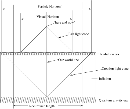
Figure 1: Creation lightcone larger than the identification scale. There are no particle horizons and all events at last scattering are causally connected.

Case 1. $\Psi_{H}(t_{eq})\geq\pi>\;2\Psi_{VH}(t_{eq}):$ all points on the LSS are in causal contact and their combined images cover the entire sky; thus the horizon problem is solved on all angular scales (see Fig. 1). There are no event horizons by the end of inflation.

While this can happen – when there is an extremely high value for $\Omega_{\Lambda}$ (much, much larger than $1$) – (25) together with realistic estimates for $c_{2}$ shows this is not true in most inflationary universes when $k=+1$. So we need to consider the situation when $\Psi_{H}(t_{eq})<\pi$. The geometry of the situation then is as follows: the visual horizon corresponds to the intersection of our past light-cone $C^{-}(E)$ with the LSS ($E$ is the point here and now) , which is a 2-sphere $\mathcal{C}_{H}$ of radius $D_{VH}(t_{eq})$ in the LSS, centered on our past world line $\gamma$. The particle horizon of any point $q$ in the LSS is a 2-sphere $\mathcal{S}_{H}$ of radius $D_{H}(t_{eq})$ in the LSS, centered on $q$, generated by the creation light cone of the observer . When $q$ is on $\gamma,$ these two spheres will be concentric. Now two cases are possible.

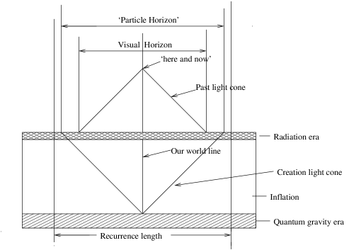
Figure 2: Creation lightcone less than the identification scale but larger than the visual horizon. There are particle horizons, but all seen events at last scattering are causally connected.

Case 2. $\pi>\Psi_{H}(t_{eq})>2\Psi_{VH}(t_{eq}):$ The horizon problem is solved in a theoretical sense when at least one photon or graviton can be interchanged between each observable point on the LSS (see Fig. 2). This will be the case if $\Psi_{H}(t_{eq})>2\Psi_{VH}(t_{eq})=2\Psi_{4},$ the factor 2 arising because we demand that points on the LSS that we see in opposite directions in the sky are able to communicate with each other (Note that these points are unable to communicate with each other, because $c_{4}<\pi/2.)$. Thus from (24,25), the requirement for solving the horizon problem in this sense is

$$\Psi_{H}(t_{eq})>\;0.24\frac{\pi}{2}\Leftrightarrow(c_{1}+c_{2}+c_{3})\approx 2c_{2}>0.24\;.$$ (27)

This is possible for some $k=+1$ inflationary models, as we see by the above analysis. 

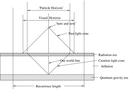
Figure 3: Creation light cone less than the identification scale and visual horizon. There are particle horizons, and not all seen events on last scattering are causally connected.

Case 3. $\pi>2\Psi_{VH}(t_{eq})>\Psi_{H}(t_{eq}):$ The horizon problem is not solved in the sense that points on the LSS that we can observe (they lie within the visual horizon) are not pairwise-causally connected to each other (see Fig. 3). This will be the case when (27) is not true, that is, when

$$c_{2}<0.12.$$ (28)

There are many $k=+1$ inflationary models for which this is true, irrespective of how many e-foldings occur; they simply have to start well away from the minimum of cosh$\lambda t$ (see (7)), which is given by $\Omega_{\Lambda}=\infty$.

IV.1 Causal Diagrams

How is this related to the usual causal diagrams Ref4a , that suggest that the horizon problem is solved by inflation pushing down the start of inflation $t=t_{i}$ arbitrarily far in those diagrams when inflation occurs? Horiz . The point here is that when $k=+1$, we can’t push the initial surface $t=t_{i}$ down arbitrarily far in those diagrams, however much inflation is allowed, because the integral (10) is bounded, see (21) above and the conformal diagrams in (Ref4a ). In analytic terms, the difference is essentially that between evaluating this integral for a de Sitter universe in a $k=0$ ($a(t)\;=expHt$) frame, when we can push the integral back to negative times as far as we like (the epoch $t=0$ being arbitrarily assigned), and evaluating it in a $k=+1$ ($a(t)=\cosh Ht)$ frame Schr , where the time $t=0$ is a preferred time (the turn-around time for the scale factor) and is the maximum to which the integral can be extended Paper_1 , see ( 8). The integral $\int dt/a(t)$ is quite different in these two cases, indeed this integral has a discontinuous limit as the spatial curvature $K(t_{o})=k/S^{2}(t_{o})$ goes to zero: for $\Omega\leq 1$, it is unbounded with unbounded integration limits, but for all $\Omega>1$, it has bounded integration limits and is bounded by the limits given above. This is possible because when $K>0$ and $\Lambda$ is indeed constant (or almost constant) the $k=+1$ term always dominates this integral eventually at early enough times, no matter how small $K$ is today (until radiation kicks in and becomes the dominant term: but that is the end of inflation). Thus given any desired number of e-foldings, evaluating the integral for $\Omega_{0}=1$ (as is usually done) gives quite a different result from evaluating it for $\Omega_{0}=1+\varepsilon$ with $\varepsilon>0,$ no matter how small $\varepsilon$ is.

IV.2 Realistic Estimates

In order to estimate how probable cases 2 and 3 are, we have examined a grid of models of the kind described above in which the inflationary epoch has at least 60 e-foldings, and is varied by allowing (i) different starting times after the end of the Planck epoch (i.e. different periods of radiation domination before inflation commences), (ii) different ending times well before the nucleosynthesis epoch but below the GUT energy, and (iii) different final values of the density parameter $\Omega_{0}$. Details are given in Paper_2 . The conclusion is that in most cases inflation will not succeed in solving the horizon problem because (27) is not true. The only cases in which inflation will solve the horizon problem are those in which it begins very close to the turn-around in the $\cosh$ function, that is at a very nearly static state and with an enormously high value for $\Omega_{\Lambda}$. The essential point is that given any chosen starting conditions, the integral (10) rapidly comes very close to its final value and thereafter no matter how much more inflation takes place, it adds a negligible amount to this integral;

V The Relation to Homogeneity

The above causal analysis gives upper limits to the scales on which causal processes can operate. But single contact by massless particles is clearly insufficient to cause homogenization; much more interaction is needed. Additionally, the effect of interactions restricts realistic causation much more. The extremely short mean free path for matter and radiation in the radiation-dominated era implies that only massless neutrinos and gravitational radiation travel at the speed of light in this epoch, and they cannot cause homogeneity; massive particles and electromagnetic radiation travel much slower. Thus effective causal interactions will come from a much more restricted domain at early times than indicated by causal horizons based on the local speed of light. This means the true horizon problem is even greater than indicated by the above estimates.

To examine this in detail, we need an estimation of the domain that causes significant effects locally in the neighbourhood of our Galaxy, as a function of time (or equivalently, of scale factor) - how large was this domain at nucleosynthesis, at baryosynthesis, at the end of inflation, at the Planck time? There are three major physical effects to consider: nucleosynthesis, smoothing and structure formation (growth of density inhomogeneities). A detailed discussion will be given in Paper_2 .

V.1 Chemical Composition: Uniform Thermal Histories

The local composition of matter depends on the relevant thermal histories of that matter, determined by local conditions near the particle world lines in the early universe. A uniform chemical composition on large scales thus depends on uniform thermal histories occurring in widely separated regions in the early universe Ref9 . The point is that while some diffusion of elements will take place after nucleosynthesis, this will be strongly damped by the expansion of the universe; neither particles nor radiation can move freely because of tight coupling between them, so element abundances set up early on will tend to stay put in the same (comoving) place. There might for example be an initial spatial variation in the baryon number density, lepton number density, and charge density, as well as in local densities and expansion rates, generating different photon-to-baryon ratios in different regions, and hence resulting in spatially varying nucleosynthesis patterns. The resulting inhomogeneous element abundances will remain unchanged in the same comoving locations until decoupling has taken place and star formation has begun.

The issue, then, is the particle horizon size at the times of nucleosynthesis and baryosynthesis, determining the limits of causality for the epochs of baryosynthesis and nucleosynthesis, and hence for resulting uniform thermal histories at later times. These scales will be more or less the same as those at the end of inflation, for which speed-of-light limits are given by $\Psi_{H}(t_{f}),$ estimated above (25); they will be seen on the surface of last scattering as in (15). From the estimates above, the implication is that in most $k=+1$ models, there will not be a possibility of setting up causally equalized conditions for nucleosynthesis by physical processes occurring during inflation. The element abundance sky will consist of many causally disconnected domains.

V.2 Smoothing by Expansion

What will take place unchanged is the smoothing out that is associated directly with expansion, which smooths out structures locally, independent of what happens at distant places. The argument is simple: choose a smooth enough domain, however small, at the end of the Planck era; enough e-foldings during inflation will make it larger than the visual horizon size at decoupling, and so will explain the observed homogeneity today. This is what is understood by many as the major causal mechanism by which inflation causes homogeneity at late times. On this scenario, the large-scale homogeneity we measure today is due to homogeneity on very small physical scales being set up prior to inflation, during the Planck epoch, so we can no longer ignore $\Psi_{Planck},$ as we have done up to now. Whether or not inflation is able to solve the horizon problem of causal connectivity is then irrelevant; the necessary homogeneity (on a very small physical scale) was created before inflation began, and then preserved when one follows the comoving evolution of inhomogeneities.

The causal implications for the Planck era are quite severe. Indeed it is clear from the relevant causal diagrams (see Fig. 4) that the essential requirement for this to succeed is that

$$\Psi_{Planck}>\Psi_{VH}=\Psi_{4}:$$ (29)

at the beginning of inflation, there was already causal connectivity on a scale larger than the scale of the entire visible universe today retrodicted to that time. When this is true, whether or not this local process in fact leads to smoothing is then totally dependent on (i) what relics are left over from the quantum gravity era at what wavelengths, and (ii) on how uniform the subsequent expansion is.

VI The quantum gravity problem

Ultimately causal estimates depend on unknown physics in the Planck era, where space-time foam, a lattice domain, or tumbling light cones may occur and determine causal connectivity at the start of inflation (Guth emphasizes that the initial size of an inflationary patch need be only one billionth the size of a single proton Ref1 .). It is certainly clear that physics in the Planck era influences initial conditions for inflation, and hence the anisotropy and inhomogeneity spectra observed today transPlanck ; what is not clear is that the almost-FL studies carried out so far give anything like the correct answer. If conditions are very inhomogeneous, almost everywhere inflation may not succeed in starting; however when it does succeed, it will soon dominate the local universe region in volume terms. In that region, inflation will dramatically amplify the comoving scales associated with whatever inhomogeneity there is to begin with. The remnants of quantum gravity may not be smooth: they may be arbitrarily inhomogeneous, even fractal - and usual inflationary studies do not consider this full range of possibilities Penrose . In contrast, some studies propose quantum mechanism that will indeed create the universe in a smooth state that solves the homogeneity problem in $k=+1$ models before inflation ever begins Linde , but as the link between quantum gravity and quantum cosmology models is not yet firmly established, this proposal must be treated with some caution.

Two principal questions we must therefore address to quantum cosmology are: 1. What processes in the Planck era were responsible for the initial causal self-connectedness and homogeneity of the primordial universe at the Planck transition (whatever its size)? and 2. What determines the limiting size of such a region – what are the limits to the correlations quantum gravitational process can establish at the Planck transition? Even if it turns out that this limit is indeed the Planck length, the first question demands an adequate answer. And, given that space and time – and therefore causality itself – would not have anywhere near the same structure in the Planck era as after the transition to classical space-time, the second question also demands careful consideration.

Thus, the fundamental problem is that we don’t know the causal connection size during the quantum gravity era nor at the Planck time. We can calculate it in a  FRW context, but that context will not obtain at very early times when quantum fluctuations in space-time structure are severe. Nevertheless, we need to estimate the Planck contribution $\Psi_{Planck}$ in order to truly understand the range of causality in the later universe. And the ‘smoothing by expansion’ proposal can only work if (29) is satisfied as a result of those processes.

VII Event Horizons

Event horizons Ref4 occur if $\Psi(E,F)\equiv\int_{t_{E}}^{t_{F}}(c/S(t))dt$ is bounded as $t(F)\rightarrow t_{\max}$. From the integral (17), this is indeed the case when if $k=+1$ and $\Lambda=0$, for then always $\Psi(1,E,F)<\pi$. If there is a cosmological constant in such models that will only make the situation worse, because such a constant by itself will always (i.e. with the single exception of the highly unstable case of a model asymptotic to an Einstein Static universe in the future) lead to this integral being bounded even if $t\rightarrow\infty$. That is, irrespective of the value of a cosmological constant, and, whether or not there is some entity like quintessence present, there will always by event horizons in $k=+1$ FL universe models. Thus the alleged problems for string theory resulting from the existence of event horizons Ref5 will always be implied by such models. This is in addition to any problems arising because the space sections are compact, so that there is no infinity to use for setting data.

However it is not clear that this would necessarily be a death-knell for string theory, even if we were eventually to conclude conclusively that $k=+1$ in the real universe. The key point here is that string theory is in essence a theory of small scale structure and quantum gravity properties, and we are here considering properties of the universe on the largest observable scales, and indeed on scales that might never be observable (c.f. Ref11 ). One might suggest that an ‘effective infinity’ for $S$-matrix calculations for string theory could be at a finite distance from a local object (for example, at CERN the ‘effective infinity’ where the outermost measurements are made is at a distance of about 10 meters from where the particle collisions take place), rather than having to be taken literally to infinity (which is way outside the visual horizon – so we have no chance of knowing what conditions are like there anyhow). Thus it may be worthwhile pursuing a somewhat more local version of the setting of data for string theory, in line with the spirit of the ‘finite infinity’ proposal in Fi .

VIII Conclusion

If the universe has positive spatial curvature $(k=+1)$, then no matter how much inflation takes place, effective causality since the Planck time is almost always smaller than the whole LSS – unless there were extreme conditions right at the beginning of inflation, that is, no significant cosmic expansion before that. The CBR intensity sky, mirroring the density fluctuations at last scattering that later led to structure formation, will usually consist of causally disconnected regions, and in these cases the same applies to the element abundance sky, mirroring the early epoch of nucleosynthesis. If inflation is going to solve the horizon problem in all cases, we must have $k=-1$ (given that $k=0$ is infinitely improbable). If $k=+1$ is observationally indicated, that will suggest that we need (in practically all cases) physical homogeneity prior to inflation, because it can be created by physical processes during inflation only in the extreme case of an enormously large (virtually infinite) $\Omega_{\Lambda}$, corresponding to virtually no cosmic expansion before inflation itself. This conclusion in fact accords with the understanding many have of inflation as simply expanding already homogenized patches of the universe, smoothed out by processes at work in the Planck era. While this may be a plausible mechanism, it is somewhat surprising to see this proposed causal structure (shown in Figure 4), based on comoving timelike world lines, given the emphasis placed in much of the inflationary literature on the way that inflation is directly able to solve the horizon problem.

It should be noted that this conclusion is based purely on examining inflation in FL universe models with a constant vacuum energy, and is not based on examinations of Trans-Planckian physics on the one hand, nor on studies of embedding such a FL region in a larger region on the other, nor does it take scalar field dynamics into account. In may be that physics in the Planck era will smooth things out on large enough comoving scales that the universe today is spatially homogeneous simply by comoving expansion; in that case the horizon problem is irrelevant. This indeed appears to be the option proposed in many inflationary studies. We suggest that in that case, this position should be made clear. Then inflation is not required to solve the causal issues raised by the horizon problem; it is the Planck era that is assumed to do so, despite the unknown physics of that era.

We do not expect any major difference from our results to occur for the case of more realistic exponential inflationary models of the early universe. But power-law inflation may give quite different answers, and one could solve the problem by models that are not slow-rolling for a major part of the scalar-field dominated early era; but then they fall outside the standard inflationary paradigm. We are fully aware that in order to properly study the issue, we need to examine anisotropic and inhomogeneous geometries rather than just FL models, because analyses based on FL models with their Robertson-Walker geometry cannot be used to analyse very anisotropic or inhomogeneous cases. Nevertheless this study shows there are major causal differences in inflationary FL universes with $k=+1$ or $k=-1,$ influencing the ability of physical processes to causally homogenise the universe. The implication is (a) that we need to try all observational methods available to determine which is the case, because this makes a significant difference not only to the spatial topology, but also to the causal structure of the universe, and (b) we should examine inhomogeneous inflationary cosmological models to see if any similar difference exists in those cases between causal behaviour of models that are necessarily spatially compact, and the rest.

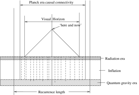
Figure 4: Causality generated by comoving expansion of world-lines. The vertical lines are comoving, and causality generated at the Plank scale is assumed to be bigger than the visual horizon. The creation light cone is irrelevant.

References

- (1) Netterfield et al.(2001): astro-ph/0104460.
- (2) Riess et al. (1998): Astron Journ. 116, 1009. Perlmutter et al (1999): Astrophys Journ 517 , 565.
- (3) Guth A H (1981), Phys Rev D23, 347. Linde A D (1990), Particle Physics and Inflationary Cosmology (Harwood, Chur). Kolb E W and Turner M S (1990), The Early Universe (Wiley, New York, 1990). For recent reviews, see Brandenberger, R. (2001): hep-th/0101119 and Guth, A. H.(2001): astro-ph/0101507.
- (4) Stompor R., at al (2001): astro-ph/015062. Wang X et al (2001): astro-ph/0105091. Douspis, M,. et al (2001): astro-ph/0105129. de Bernadis, P., et al. (2001): astro-ph/0105296.
- (5) Ellis G F R (1987). Astrophysical Journal 314, 1.
- (6) White M and Scott D (1996). Astrophys Journ 459, 415.
- (7) Ellis GFR Stoeger W McEwan P and Dunby P (2001). ‘Dynamics of Inflationary Universes with Positive Spatial Curvature”. Preprint.
- (8) Rindler W (1956). Mon Not Roy Ast Soc 116, 662.
- (9) Penrose R. in Relativity Groups and Topology , Eds. C M DeWitt and B S DeWitt (Gordon and Breach, New York, 1963). Hawking S W and Ellis G F R (1973). The Large Scale Structure of Spacetime. (Cambridge University Press). Tipler, F., Clarke, C.J.S., and Ellis, G.F.R. (1980). In General Relativity and Gravitation: One Hundred Years after the Birth of Albert Einstein, Vol. 2, Ed. A Held (Plenum Press, New York).
- (10) Fischler W et al (2001): hep-th/0104181.
- (11) He X-G (2001): astro-ph/0105005. Cline J M (2001): hep-ph/0105251. Kolda C and Lahneman W (2001): hep-ph/0105300.
- (12) P McEwan, W Stoeger, P Dunsby, and G F R Ellis (2001): in preparation.
- (13) Weinberg S (1972). Gravitation and Cosmology (Wiley, New York).
- (14) Ellis G F R (1987), in Vth Brazilian School on Cosmology and Gravitation, Ed. M Novello (World Scientific, Singapore).
- (15) Schroedinger E (1956). Expanding Universes (Cambridge University Press, Cambridge).
- (16) Ellis G F R and Stoeger W R, (1988). Class Qu Grav 5, 207.
- (17) Bergström L and Goobar A (1999). Cosmology and Astroparticle Physics (Wiley and Sons, Chichester).
- (18) Brandenberger R (2001), hep-th/0101119; Easther R. et al (2001), hep-th/0104102; Starobinsky A A (2001), astro-ph/0104043 [the latter in fact proves the opposite to what is claimed in the title: for in it, observational constraints are used to rule out a set of trans-Planckian possibilities].
- (19) Penrose R (1989). Ann New York Acad Sci 571, 249.
- (20) Linde A (1995). Phys Lett B, 351, 99.
- (21) Ellis G F R (1971) Gen Rel Grav 2 , 7. Ellis G F R and Schreiber G (1986). Phys. Lett. 115A, 97. Lachièze Rey M and Luminet J.-P (1995). Phys Rep 254, 135.
- (22) Ellis G F R (1984). In General Relativity and Gravitation (GR10 Proceedings), ed B Bertotti et al. (Reidel, 1984); Ellis G F R (2001): gr-qc/0102017; Ellis G F R and Hogan P A (1991). Annals of Physics 210, 178.
- (23) Gomero G I, Reboucas M J, and Tavakol R (2001), gr-qc/0105002.
- (24) Kantowski R (1988). Astrophys Journ 507 . astro-ph/9802208.
- (25) Bonnor W B and Ellis G F R (1986). Mon Not Roy Ast Soc 218, 605.
- (26) Ellis G F R (1971), in General Relativity and Cosmology, Proceedings of the XLVII Enrico Fermi Summer School, Ed. R K Sachs (Academic Press, New York).