Hoop conjecture for colliding black holes :
non-time-symmetric initial data

Abstract

The hoop conjecture is well confirmed in momentarily static spaces, but it has not been investigated systematically for the system with relativistic motion. To confirm the hoop conjecture for non-time-symmetric initial data, we consider the initial data of two colliding black holes with momentum and search an apparent horizon that encloses two black holes. In testing the hoop conjecture, we use two definitions of gravitational mass : one is the ADM mass and the other is the quasi-local mass defined by Hawking. Although both definitions of gravitational mass give fairly consistent picture of the hoop conjecture, the hoop conjecture with the Hawking mass can judge the existence of an apparent horizon for wider range of parameters of the initial data compared to the ADM mass.

I introduction

The concept of an apparent horizon is very important to understand the global feature of spacetimes because the formation of an apparent horizon implies the existence of an event horizon outside of it, and a black hole has formed. Hence it is of great interest to investigate the condition for the apparent horizon formation. But the necessary and sufficient condition for the existence of an apparent horizon is not precisely understood so far. Although one theorem that gives a sufficient condition for the apparent horizon formation was proved by Schoen and Yau SY , it cannot be applicable to vacuum spaces, and it does not give a necessary condition. As one possibility to give a necessary and sufficient condition for the black hole formation, there is the hoop conjecture MWM . The conjecture states that for a spacelike hypersurface $\Sigma$, a black hole horizon exists if and only if the mass $M$ of the system gets compacted into the interior of a closed surface S whose circumference (hoop) $C$ satisfies the condition

$$H\equiv\frac{C}{4\pi M}\lesssim 1.$$ (1)

Its physical meaning is that the mass concentration in all direction is essential for the formation of a horizon, and the ratio $H$ is a parameter to judge the horizon formation.

It is meaningful to confirm the hoop conjecture not only because it is interesting theoretically, but also it can be a useful tool to test the formation of a black hole in numerical simulations. If we want to know whether a black hole has formed, we must solve a differential equation that determines the location of apparent horizons. If the hoop conjecture is correct, we can judge the black hole formation by calculating the hoop $C$ and the mass $M$ and then taking their ratio. Therefore the hoop conjecture has a possibility to give an easier method to judge the black hole formation.

Several tests of the hoop conjecture has been done by various authors. Shapiro and Teukolsky ST calculated the gravitational collapse of collisionless gas spheroids numerically. They found that when a naked singularity appears, the ratio $H$ becomes greater than $1$ and when an apparent horizon forms, $H$ takes a value close to $1$. Nakamura et al. NST investigated an analytic series of the initial data for momentarily static dust spheroids. Their result shows that there does not exist a critical value $H$ that gives both the necessary and the sufficient condition for the apparent horizon formation. Nevertheless, they indicated that there exist two characteristic values of $H$ ; the larger one gives the necessary condition and the smaller one gives the sufficient condition for the horizon formation. This means that the value of $H$ can still be a useful parameter for the apparent horizon formation. Other tests with momentarily static initial data also show $H$ is a parameter for the horizon formation AHST ; CNNS ; Chiba , and they support the hoop conjecture.

In this paper, we concentrate on the test of the hoop conjecture using initial data of Einstein’s equation. Although there are several tests of the hoop conjecture, its validity for non-time-symmetric initial data has not been systematically investigated. We pay attention to the effect of the motion of gravitational bodies on the apparent horizon formation. We prepare the initial data of colliding black holes with equal mass and equal linear momentum. We use the solution obtained by Bowen and York BY . The initial data depends on two parameters : one is a separation $L$ of two black holes and the other is a momentum $P$ of each black hole. In the momentarily static case, it is well known that the decrease of the separation $L$ of two black holes causes the formation of an apparent horizon that envelopes both black holes. It is this horizon that we concentrate on in this paper. We search the parameters $L$ and $P$ that lead to the formation of an apparent horizon.

In testing the hoop conjecture, we must specify the definition of the circumference $C$ and the mass $M$. As the circumference $C$ of the hoop, Chiba et al. CNNS has proposed the appropriate definition for all $S^{2}$ surfaces. As the definition of the mass $M$, the ADM mass is adopted usually NST ; AHST ; CNNS ; Chiba . But intuitively, the formation of an apparent horizon occurs if the mass $M$ of the system is concentrated in a sufficiently small region. The ADM mass represents the total energy of the system and we expect that $H$ given by the ADM mass becomes a good parameter to judge the horizon formation only if the energy of the system is well concentrated in a region enclosed by a some compact surface S on which the circumference $C$ is evaluated. When a lot of energy is distributed outside the surface S, the ADM mass does not give a correct gravitational mass contained interior of the surface S and is not suitable for testing the hoop conjecture.

Actually, if the ADM mass is used, we have some examples that $H$ is not a good parameter for the horizon formation. One example is a charged star B , for which $H$ can take a value close to $0.5$ even if an apparent horizon does not exist. Flanagan F suggested that one should use “quasi-local mass” that extract gravitational energy contained interior of a closed surface, because the energy of electric field distributes outside the surface of a star. In fact, if we use quasi-local mass, we can show that $H$ becomes larger than unity for such an equilibrium star. As one cannot uniquely determine the local energy in general relativity, there are many definitions of quasi-local mass. We do not know what quasi-local mass is best for the hoop conjecture. In the case of a charged star, the definitions of the quasi-local mass due to Hawking H and Penrose P ; T give better results than the ADM mass. Another example is the Brill wave spacetime AHST . In this case, the gravitational energy cannot be localized so much. If we consider the Brill wave with large width, $H$ given by the ADM mass cannot be a good parameter to judge the horizon formation AHST . These two examples indicates that $H$ given by the quasi-local mass becomes a good parameter to judge the horizon formation.

For the Bowen-York initial data, Jansen et al. JDKN discussed that this space is not a pure black hole system. They calculated the mass and the scalar invariants of the Bowen-York initial data and compared them with those of the boosted Schwarzschild black hole initial data. Their result shows that the Bowen-York initial data for the moving black hole system contains a junk gravitational field at large distances from black holes. Hence, we expect that $H$ with the quasi-local mass can be a better parameter than $H$ with the ADM mass.

In this paper, we calculate $H$ using two different definition of the mass: the ADM mass and the quasi-local mass. As the quasi-local mass, we use Hawking’s quasi-local mass H because for spherically symmetric spaces, $H$ given by the Hawking mass has a critical value $H=1$ for the horizon formation ; if $H\leq 1$, there exists a horizon and if $H>1$, there is no apparent horizon. Thus $H$ given by the Hawking mass is a critical parameter for the horizon formation as far as the spherically symmetric cases are concerned. For axially symmetric cases, we expect that this desirable feature of the Hawking mass will hold. Even there is no critical value, we regard $H$ as a parameter to judge the horizon formation if there exist two values $H_{1}$ and $H_{2}$ ; for $H<H_{1}$, an apparent horizon exists and for $H>H_{2}$, an apparent horizon does not exist. Once $H$ are obtained as functions of the parameters $L$ and $P$, we can define two regions in the parameter space $(L,P)$:

$$\mathcal{R}_{1}\equiv\{(L,P)|~{}H(L,P)<H_{1}\},$$

$$\mathcal{R}_{2}\equiv\{(L,P)|~{}H(L,P)>H_{2}\}.$$ (2)

We compare the regions $\mathcal{R}_{1,2}$ for the ADM mass with those for the Hawking mass. If $\mathcal{R}_{1,2}(\rm{ADM})\subset\mathcal{R}_{1,2}(\rm{Hawking})$, we can say that $H$ with the Hawking mass is better than $H$ with the ADM mass because the former predict wider range of the initial data parameter on the existence of the apparent horizon.

This paper is organized as follows. In Section II, we explain the method of our analysis of the two black hole initial data. In Section III, we investigate the hoop conjecture for two black holes by estimating the ADM mass and the Hawking’s quasi-local mass. Section IV is devoted to summary and discussion. We adopt the units of $c=G=1$.

II Initial data for two black holes

II.1 Initial value equations and apparent horizons

Let $\Sigma$ be a spacelike hypersurface with the intrinsic three metric $h_{ij}$ and the extrinsic curvature $\mathcal{K}_{ij}$. The initial value equations for a vacuum space are

$${}^{(3)}R-h^{im}h^{jn}\mathcal{K}_{ij}\mathcal{K}_{mn}+\mathcal{K}^{2}=0,$$ (3)

$$~{}D^{i}(\mathcal{K}_{ij}-h_{ij}\mathcal{K})=0,$$ (4)

where ${}^{(3)}R$ is the Ricci scalar of the spacelike hypersurface $\Sigma$, $\mathcal{K}$ is the trace of the extrinsic curvature and $D_{i}$ is the induced covariant derivative on $\Sigma$. We assume that the space is conformally flat and maximally sliced:

$$h_{ij}=\Psi^{4}f_{ij},\quad\mathcal{K}=0,$$ (5)

where $f_{ij}$ is the flat space metric. Taking $\mathcal{K}_{ij}=\Psi^{-2}K_{ij}$, the initial value equation becomes

$$\partial^{2}\Psi=-\frac{1}{8}K^{ij}K_{ij}\Psi^{-7},$$ (6)

$$\partial^{i}K_{ij}=0,$$ (7)

where $\partial_{i}$ is the partial derivative of a flat space and $\partial^{2}$ is the flat space Laplacian. We use the solution of Eq. (7) obtained by Bowen and York BY :

$$K_{ij}=\frac{3}{2r^{2}}[P_{i}n_{j}+P_{j}n_{i}-\left(\delta_{ij}-n_{i}n_{j}\right)P^{k}n_{k}]~{},$$ (8)

where $n^{i}=x^{i}/r$ and $P^{i}$ is the linear momentum defined by

$$P_{i}=\frac{1}{8\pi}\int_{r\rightarrow\infty}(\mathcal{K}_{ij}N^{j}-\mathcal{K}N_{i})dS.$$ (9)

Because Eq. (7) is a linear equation, one can get a solution for two black holes with momentum by superposing the solution (8) as

$$K_{ij}=K_{ij}^{(+)}+K_{ij}^{(-)},$$ (10)

$$K_{ij}^{(\pm)}=\frac{3}{2r^{(\pm)}{}^{2}}[P_{i}^{(\pm)}n_{j}^{(\pm)}+P_{j}^{(\pm)}n_{i}^{(\pm)}-\left(\delta_{ij}-n_{i}^{(\pm)}n_{j}^{(\pm)}\right)P^{(\pm)k}n_{k}^{(\pm)}].$$ (11)

The location of each black hole is $(0,0,\pm L)$ and

$$P_{i}^{(\pm)}=\left(0,0,\mp P\right),\quad n_{i}^{(\pm)}={\left(x,y,z\mp L\right)}/{r^{(\pm)}},$$ (12)

where $r^{(\pm)}=\sqrt{x^{2}+y^{2}+(z\mp L)^{2}}$. For the collision of black holes, $P$ is positive. Eq.(6) can be rewritten as the form of integral equation

$$\Psi=1+\frac{M_{0}}{4r^{(+)}}+\frac{M_{0}}{4r^{(-)}}+\frac{1}{4\pi}\int\frac{K^{ij}K_{ij}\Psi^{-7}}{8|\boldsymbol{r}-\boldsymbol{r}^{\prime}|}d\boldsymbol{r}^{\prime}{}^{3}.$$ (13)

For $P=0$, this expression reduces to the solution of the Brill-Lindquist two black hole initial data that has two Einstein-Rosen bridges BL . Each singular point $r^{(\pm)}=0$ corresponds to the asymptotically flat region. Thus the solution of Eq. (13) represents a space with three asymptotically flat regions. We use this expression to specify the boundary condition at $r^{(\pm)}=0$. For sufficiently small value of $r^{(\pm)}$, Eq.(13) reduces to

$$\Psi\approx C+\frac{M_{0}}{4r^{(\pm)}},$$ (14)

and the boundary condition at $r^{(\pm)}=0$ can be written

$$\frac{d\Psi}{dr^{(\pm)}}=-\frac{M_{0}}{4r^{(\pm)}{}^{2}}\quad\text{as}\quad r^{(\pm)}\rightarrow 0.$$ (15)

We introduce a small cut off parameter $r^{(\pm)}_{\text{cut}}=L/\cosh(10)\approx 10^{-4}L$ to impose the boundary condition at $r^{(\pm)}=0$ in numerical integration. By using a different value of cut off parameter $r^{(\pm)}_{\text{cut}}=L/\cosh(9)$, we estimated the numerical error due to the cut off is $0.03\%$. The other boundary condition is

$$\frac{\partial\Psi}{\partial\rho}\Big{|}_{\rho=0}=\frac{\partial\Psi}{\partial z}\Big{|}_{z=0}=0,$$ (16)

where $\rho=\sqrt{x^{2}+y^{2}}$. This comes from the axial symmetry about $z$-axis and the mirror symmetry about the equatorial plane. We solve Eq. (6) numerically with these boundary conditions by a finite difference method with $160\times 100$ grids in bispherical coordinates. By comparing the calculation with $320\times 200$ grids, we estimate the numerical error is about $0.2\%$.

Once the initial data are obtained, we search apparent horizons for the initial data. The apparent horizon is a $S^{2}$ surface on which the expansion of the outgoing null geodesic congruence normal to it vanishes. Let $s^{a}$ be a unit vector tangent to $\Sigma$ and normal to a two-dimensional spacelike surface and $n^{a}$ be a unit vector normal to $\Sigma$. Then $k^{a}=n^{a}+s^{a}$ is a future directed and outward pointing null vector on the surface. This surface is an apparent horizon if the condition

$$\theta_{+}=\nabla_{a}k^{a}=D_{a}s^{a}-K+K_{ab}s^{a}s^{b}=0$$ (17)

is satisfied. We rewrite this equation with spherical coordinates $(r,\theta,\phi)$. By expressing the $S^{2}$ surface as $r=h(\theta)$, Eq. (17) becomes

$$h_{,\theta\theta}-\left(4\frac{\Psi_{,r}}{\Psi}+\frac{2}{h}\right)h^{2}-\left(4\frac{\Psi_{,r}}{\Psi}+\frac{3}{h}\right)h_{,\theta}^{2}+\left(4\frac{\Psi_{,\theta}}{\Psi}+\cot\theta\right)h_{,\theta}\left(1+\frac{h_{,\theta}^{2}}{h^{2}}\right)\\ -h^{2}\left(1+\frac{h_{,\theta}^{2}}{h^{2}}\right)^{1/2}\frac{1}{\Psi^{4}}\left(K_{rr}-2\frac{h_{,\theta}}{h^{2}}K_{r\theta}+\frac{h_{,\theta}^{2}}{h^{4}}K_{\theta\theta}\right)=0.$$ (18)

We solve this equation with the boundary condition $h_{,\theta}=0~{}\text{at}~{}\theta=0,\pi/2$.

II.2 Circumference, ADM mass and Hawking mass

In axially symmetric spaces, the circumference $C$ of a surface S is defined by

$$C(\text{S})={\text{max}}(L_{e},L_{p}),$$ (19)

where $L_{e}$ is the maximum length of closed azimuthal curves and $L_{p}$ is the twice of the distance from the north pole to the south pole. We survey all surfaces S which enclose two black holes. Because the circumference can become arbitrarily large, we must calculate the minimum value $H$ of $H(\rm{S})$ for all surfaces S.

We write $H$ given by the ADM mass as $H^{(\rm{A})}$ hereafter. Searching the minimum value $H^{(\rm{A})}$ of $H^{(\rm{A})}(S)$ corresponds to finding the surface with the minimum value of $C$ because the ADM mass is defined independent of the surface S. For our initial data, $L_{e}<L_{p}$ is always satisfied and we have

$$C=L_{p}=2\int^{\pi}_{0}\Psi^{2}\sqrt{{h_{,\theta}}^{2}+h^{2}}\,d\theta~{},$$ (20)

where we express the surface as $r=h(\theta)$. We obtain the equation to determine the hoop length by taking variation of this integral $\delta C=0$ :

$$h_{,\theta\theta}-\left(2\frac{\Psi_{,r}}{\Psi}+\frac{1}{h}\right)h^{2}-\left(2\frac{\Psi_{,r}}{\Psi}+\frac{2}{h}\right)h_{,\theta}^{2}+2\frac{\Psi_{,\theta}}{\Psi}h_{,\theta}\left(1+\frac{h_{,\theta}^{2}}{h^{2}}\right)=0.$$ (21)

We solve this equation with the boundary condition $h_{,\theta}=0$ at $\theta=0,\pi/2$. The ADM mass in a conformally flat space is defined as follows:

$$M_{\rm{ADM}}=-\frac{1}{2\pi}\int_{r\rightarrow\infty}\partial_{i}\Psi N^{i}dS~{},$$ (22)

where $N^{i}$ is a unit outward normal to a spherical surface at infinity. Using the Gauss law and the boundary condition at $r^{(\pm)}=0$, we get

$$M_{\rm{ADM}}=M_{0}+\frac{1}{2\pi}\int\frac{1}{8}K^{ij}K_{ij}\frac{1}{\Psi^{7}}d\boldsymbol{r}^{\prime}{}^{3}.$$ (23)

We also calculate the minimum value $H^{(\rm{H})}$ of $H^{(\rm{H})}(\rm{S})$ with the Hawking mass. The Hawking mass $M_{\rm{H}}(\rm{S})$ inside the surface S is defined by

$$M_{\rm{H}}(\text{S})=\frac{S^{1/2}}{(4\pi)^{3/2}}\left(2\pi+\frac{I(\rm{S})}{8}\right),$$ (24)

where $I({\rm{S}})=\int_{{\rm{S}}}\theta_{+}\theta_{-}dS$ and $S$ is the area of the surface S. $\theta_{+}$ and $\theta_{-}$ are the expansion for the outgoing and the ingoing null congruence on S, respectively. The minimum value $H^{\rm{(H)}}$ of $H^{(\rm{H})}(\rm{S})$ is expressed as

$$H^{\rm{(H)}}=\frac{C}{4\pi M_{H}}=\frac{C}{\sqrt{\pi S}}\left(1+\frac{I}{16\pi}\right)^{-1}$$ (25)

where $C$ and $S$ are evaluated on the surface $\rm{S}_{\rm{min}}$ that gives the minimum value of $H^{(\rm{H})}(\rm{S})$ and $I\equiv I(\rm{S}_{\rm{min}})$.

We expand the equation of the surface $r=h(\theta)$ by using Legendre’s polynormals:

$$h(\theta)=a_{0}+a_{2}P_{2}(\cos\theta)+a_{4}P_{4}(\cos\theta)+\cdots.$$ (26)

We truncate the series with some finite number $l_{c}$ and find the coefficient $a_{l}~{}(l=0,2,\cdots,l_{c})$ that make the value $H^{(\rm{H})}(\rm{S})$ minimum. We used $l_{c}=4$. By using the different value $l_{c}=2$, we estimated that the maximal numerical error is less than $0.1\%$.

III Numerical results

FIG. 1 shows the parameter $(L,P)$ of the initial data that the apparent horizon exists. Even for large separation $L$ of two black holes, an apparent horizon can exist provided that the momentum $P$ is sufficiently large. We call the boundary of these two regions as a critical line $P=P_{\rm{crit}}(L)$. The critical line intersects the $L$-axis at $L=0.383M_{0}$. The line $P=9.8L$ is an asymptote of the critical line for $1\ll L/M_{0}$ and $1\ll P/M_{0}$. Cook et al. C also obtained a critical line for two colliding black holes in a similar setting. He used the Misner-Lindquist type initial data with two Einstein-Rosen bridges and two asymptotically flat regions. He also got the result that the motion of two black holes helps the horizon formation in the colliding case.

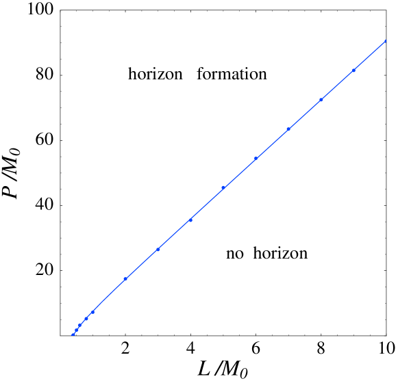
Figure 1: The parameter space $(L,P)$ of the initial data. For the parameters in the upper region, an apparent horizon that encloses the two black holes exists. The momentum $P$ helps the formation of the horizon. Two regions are separated by the critical line.

Now we test the hoop conjecture with the ADM mass. FIG. 2 shows the contour lines of $H^{(\rm{A})}$ in the $(L,P)$-plane.

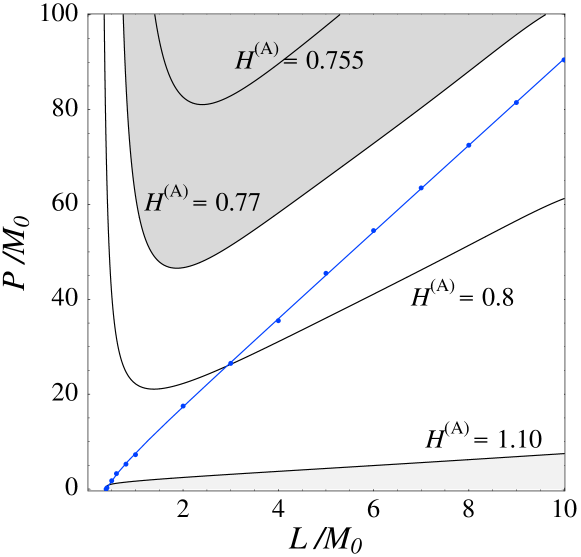
Figure 2: The contour lines of $H^{(\rm{A})}=C/(4\pi M_{\text{ADM}})$. For the initial data with parameters in the light gray region ($1.10<H^{(\rm{A})}$), there is no apparent horizon. For the initial data with parameters in the dark gray region ($H^{(\rm{A})}<0.77$), an apparent horizon always exists. We have two values $H_{1}^{(\rm{A})}=0.77$ and $H_{2}^{(\rm{A})}=1.10$.

The contour line with $H^{(\rm{A})}=1.10$ becomes a tangent line of the critical line near $(L,P)\sim(0.4M_{0},0)$. We can observe that the apparent horizon never exists for $1.10<H^{(\rm{A})}$ and we have $H^{(\rm{A})}_{2}=1.10$. For large $L$ and $P$, the contour line with $H^{(\rm{A})}=0.77$ becomes an asymptote of the critical line. For $H^{(\rm{A})}<0.77$, a black hole horizon always exists and we have $H^{(A)}_{1}=0.77$.

Next, we calculate the value $H^{(\rm{H})}$ using the Hawking’s quasi-local mass. The result is shown in FIG. 3.

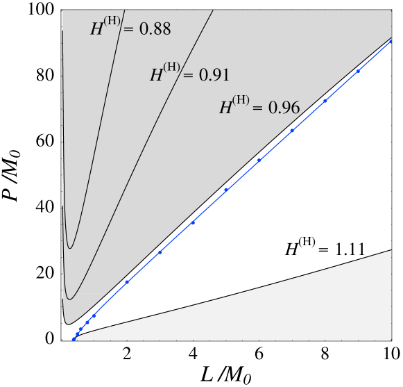
Figure 3: The contour lines of $H^{(\rm{H})}=C/(4\pi M_{\text{H}})$. For the initial data with parameters in the light gray region ( $1.11<H^{(\rm{H})}$), there is no horizon. For the initial data with parameters in the dark gray region ($H^{(\rm{H})}<1.11$), an apparent horizon always exists. We have two values $H_{1}^{(\rm{H})}=0.96$ and $H_{2}^{(\rm{H})}=1.11$.

The contour line with $H^{(\rm{H})}=1.11$ is a tangent line of the critical line near $(L,P)\sim(0.4M_{0},0)$. The apparent horizon never exists for $1.11<H^{(\rm{H})}$ and we have $H^{(\rm{H})}_{2}=1.11$. For large $L$ and $P$, the contour line with $H^{(\rm{H})}=0.96$ becomes an asymptote of the critical line. For $H^{(\rm{H})}<0.96$, a horizon always exists and we have $H^{(\rm{H})}_{1}=0.96$.

In both cases that we use the ADM mass and the Hawking mass, we obtain two values $H_{1}$ and $H_{2}$, and the ratio $H$ is related to the existence of the horizon. As the kinetic energy due to the colliding motion of black holes increases the rest mass of the system, the increase of the momentum $P$ results in the increase of the mass. This leads to the decrease of $H$ in accordance with the horizon formation. In the $(L,P)$-plane, the region $H^{(\rm{H})}<H^{(\rm{H})}_{1}$ contains the region $H^{(\rm{A})}<H^{(\rm{A})}_{1}$, and the region $H^{(\rm{H})}_{2}<H^{(\rm{H})}$ contains the region $H^{(\rm{A})}_{2}<H^{(\rm{A})}$. Hence $H^{(\rm{H})}$ is superior to $H^{(\rm{A})}$ because there are some cases that we can judge the existence of a horizon by using $H^{(\rm{H})}$ but cannot judge it by using $H^{(\rm{A})}$.

We explain the reason why $H^{(\rm{H})}$ is the better parameter for the horizon formation compared to $H^{(\rm{A})}$ as follows. The Bowen-York initial data for two black holes contains a lot of gravitational wave mode which is not localized so much. The ADM mass evaluates not only the gravitational energy that is the source to make a black hole horizon, but also the gravitational energy that does not contributes to the horizon formation. As the Hawking mass gives proper gravitational mass, $H^{(\rm{H})}$ gives a better picture of the hoop conjecture compared to $H^{(\rm{A})}$.

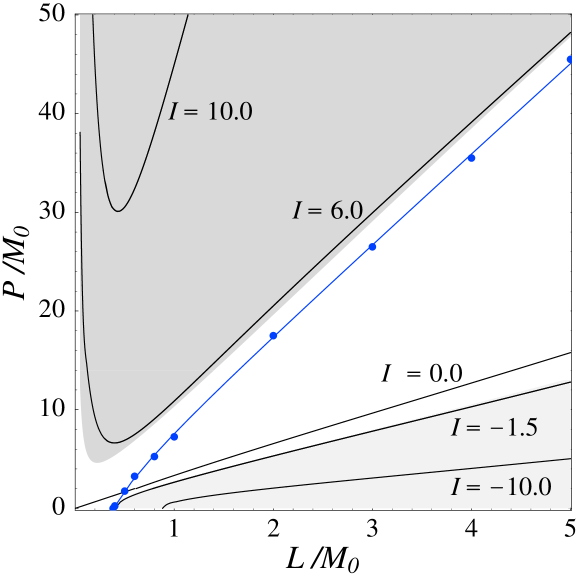
Figure 4: The contour lines of the integral $I=\int_{\text{S}}\theta_{+}\theta_{-}dS$ in the Hawking mass. The regions $H^{(\textrm{H})}_{2}<H^{(\textrm{H})}$ (light grey region) and $H^{(\textrm{H})}<H^{(\textrm{H})}_{1}$ (dark grey region) are also shown.

In introduction, we stated that $H^{\rm{(H)}}$ has a critical value for the horizon formation in the spherically symmetric case and it is the desirable feature of $H^{(\rm{H})}$. For the spherically symmetric spaces, $C/\sqrt{\pi S}=1$ and Eq. (25) becomes $H^{(\rm{H})}=(1+I/16\pi)^{-1}$. If we restrict our attention to the spherically symmetric space without white hole regions, $\theta_{-}$ is negative for all surfaces S. Because $I(\textrm{S})=\int_{\textrm{S}}\theta_{+}\theta_{-}dS=\theta_{+}\theta_{-}S$, the sign of $I(\rm{S})$ is opposite to the sign of $\theta_{+}$ on S. If there is no apparent horizon, $\theta_{+}>0$ and $I(\rm{S})<0$ for all surfaces S. Thus $I$ is negative and $H^{(\rm{H})}$ becomes greater than unity. If there is an apparent horizon, there exists a surface S on which $\theta_{+}\leq 0$ and $I(\rm{S})\geq 0$. Thus $I\geq 0$ and $H^{(\rm{H})}$ becomes smaller than unity. Therefore in the spherically symmetric cases, the sign of $I$ exactly corresponds to the existence of an apparent horizon and $H^{(\rm{H})}$ becomes a critical parameter for the horizon formation.

In the two black hole case, the factor $C/\sqrt{\pi S}$ in Eq. (25) varies in the range $1.0\leq C/\sqrt{\pi S}\leq 1.1$ for the parameters $(L,P)$ that we have investigated. Hence the value of $H^{\rm{(H)}}$ depends mainly on the value of $I$. The contour lines of $I$ in the $(L,P)$-plane is shown in FIG. 4. The line with $I=0$ that can be approximated as $P=3.2L$ crosses the critical line. In contrast to the case of the spherical collapse, the sign of $I$ does not exactly corresponds to the existence of a horizon. There exist parameter regions that $I<0$ with a horizon and $I>0$ without a horizon. In $P=0$ case, $\theta_{+}=-\theta_{-}$ holds on S and $I$ always becomes negative, even there is a horizon. Because $I$ depends continuously on parameters $L$ and $P$, there is a region $P_{\rm{crit}}(L)<P<3.2L$ where $I<0$ with a horizon. By the equation (25), this negative $I$ implies that $H^{\rm{(H)}}>{C}/{\sqrt{\pi S}}>1$. Thus there is a region in $(L,P)$-plane where $H^{\rm{(H)}}$ takes the value greater than $1$ but there is a horizon. For the initial data with parameters $3.2L<P<P_{\rm{crit}}(L)$, a horizon does not exist and there is no surface on which $\theta_{+}\theta_{-}$ keeps positive definite value. But the sign of the integral $I$ is positive. This is because for non-time-symmetric initial data, it is possible to make a surface on which $\theta_{+}\theta_{-}$ changes its sign. Thus there exists a surface S that satisfy $I(\text{S})>0$ even there is no horizon. On the surface $\rm{S}_{\rm{min}}$, $\theta_{+}\theta_{-}$ is positive near the poles and this makes the integral $I$ positive. In the region $3.2L<P<P_{\rm{crit}}(L)$, $I$ takes a value up to $6.0$ . For $I\simeq 6$, $H^{(\rm{H})}\simeq 0.89C/\sqrt{\pi S}<1$. This is the reason why there is the parameter region that $H^{(\text{H})}$ takes the value less than unity but the apparent horizon does not exist.

In the two black hole case, the sign of $I$ does not exactly correspond to the existence of a horizon. A horizon exists if $I>6$, and a horizon does not exist if $I<-1.5$. These correspond to the values $H^{\rm{(H)}}_{1}=0.96$ and $H^{\rm{(H)}}_{2}=1.11$. Contrary to the spherically symmetric case, $H^{(\rm{H})}$ does not have a critical value for the horizon formation in the axially symmetric case. But $H^{(\rm{H})}$ is the better parameter than $H^{(\rm{A})}$ to judge the horizon formation.

IV Summary and discussion

In the context of the hoop conjecture, we investigated the condition for the apparent horizon formation for two colliding black holes. The motion of black holes helps the formation of the horizon. We tested the hoop conjecture using the ADM mass and the Hawking mass. Although in both cases the ratio $H$ is related to the existence of the horizon, $H^{(\rm{H})}$ is superior to $H^{(\rm{A})}$ for the purpose of judging the existence of the horizon.

In this paper, we considered the two black hole system only in colliding case. We have also investigated the receding case $P<0$. When two black holes are receding, the motion prevents the formation of the black hole horizon. But with the increase of $|P|$, the value $H$ decreases and we have no value $H_{1}$. This behavior of $H$ shows that the ratio $H$ is not a parameter for the black hole formation in the receding case. However in the receding case, $H$ is related to the formation of a white hole horizon on which $\theta_{-}=0$. Combining the colliding and the receding cases, we can say that $H$ is a parameter of either the black hole formation or the white hole formation.

In the receding case, if a black hole horizon exists, it is located in a white hole region. Even S is in a black hole region, $I(\rm{S})$ becomes negative because $\theta_{+}<0$ and $\theta_{-}>0$ are satisfied on S. Thus the sign of $I$ scarcely corresponds to the existence of the black hole horizon. This is the reason why $H^{(\rm{H})}$ cannot be a parameter for the black hole formation in the receding case. Similarly, in spherically symmetric case, $H^{(\rm{H})}$ cannot be a parameter for the black hole horizon formation if white hole horizon exists outside of it.

The formation of a black hole occurs as the result of the temporal evolution of the initial data, and a black hole horizon in a white hole region may not be realized by the process of usual gravitational collapse if the initial data does not contain white hole regions. As far as the physically realizable situation is concerned, we expect that $H^{(\rm{H})}$ is a good parameter to judge the black hole formation.

References

- (1) R. Schoen and S. T. Yau, Commun. Math. Phys. 90, 575 (1983).
- (2) K. S. Thorne, in Magic without Magic: John Archbald Wheeler, edited by J.Klauder (Freeman, San Francisco, 1972).
- (3) S. L. Shapiro and S. A. Teukolsky, Phys. Rev. Lett. 66, 994 (1991).
- (4) T. Nakamura, S. L. Shapiro and S. A. Teukolsky, Phys. Rev. D 38, 2972 (1988).
- (5) A. M. Abrahams, K. R. Heiderich, S. L. Shapiro and S. A. Teukolsky, Phys. Rev. D 46, 2452 (1992).
- (6) T. Chiba, T. Nakamura, K. Nakao and M. Sasaki, Class. Quantum. Grav.11, 431 (1994).
- (7) T. Chiba, Phys. Rev. D 60, 044003 (1999).
- (8) J. M. Bowen and J. W. York, Jr., Phys. Rev. D 21, 2047 (1980).
- (9) N. Jansen, P. Diener, A. Khokhlov, and I. Novikov, gr-qc/0103109 (2001).
- (10) W. B. Bonnor, Phys. Lett. 99A, 424 (1983).
- (11) E. Flanagan, Phys. Rev. D 44, 2409 (1991).
- (12) S. Hawking, J. Math. Phys. 9, 598 (1968).
- (13) R. Penrose, Proc. R. Soc. London A381, 53 (1982).
- (14) K. P. Tod, Proc. R. Soc. London A388, 457 (1983).
- (15) D. R. Brill and R. W. Lindquist, Phys. Rev. 131, 471 (1963).
- (16) G. B. Cook and A. M. Abrahams, Phys. Rev. D 46, 702 (1992).