[

Density Discontinuity of a Neutron Star and Gravitational Waves

Hajime Sotani1 Electronic address:sotani@gravity.phys.waseda.ac.jp    Kazuhiro Tominaga1 Electronic address:tominaga@gravity.phys.waseda.ac.jp    and Kei-ichi Maeda1,2 Electronic address:maeda@gravity.phys.waseda.ac.jp 1 Department of Physics, Waseda University, 3-4-1 Okubo, Shinjuku, Tokyo 169-8555, Japan 2 Advanced Research Institute for Science and Engineering,
Waseda University, Shinjuku, Tokyo 169-8555, Japan
Abstract

We calculate quasi-normal f- and g-modes of a neutron star with density discontinuity, which may appear in a phase transition at extreme high density. We find that discontinuity will reflect largely on the f-mode, and that the g-mode could also be important for a less massive star.

pacs:
PACS number(s): 04.25.Nx, 04.30.-w, 04.40.Dg

]

I Introduction

Gravitational wave interferometers such as LIGO, VIRGO, GEO600, and TAMA300 on earth, and LISA in space [1] are almost ready to observe directly the gravitational waves from the Universe. The significance of direct observation of gravitational waves is that we obtain new method to observe the Universe by gravitational waves (the so-called gravitational wave astronomy), and that we may be able to verify the theory of gravity, and that new physics at high density or high energy region can be found by observing a merger of a binary neutron star.

The one of the sources of the gravitational waves is supposed to be supernova explosion, which occurs at the last phase of a massive star. After explosion, a newly formed compact object may oscillate violently, and the emitted gravitational waves carry the information of the sources. The oscillation will eventually damp out because that the gravitational waves carry the energy. The merger of two coalescing black holes or neutron stars is another source. It is naturally expected that the final object will also oscillate. If a final compact object is a neutron star, its structure will reflect on the emitted gravitational waves. There should be some relation between a structure of a neutron star and the emitted gravitational waves. The structure of a neutron star not yet well-known because the equation of state is uncertain at the high density over the nuclear density. Therefore, although main composition of matter in a neutron star is neutron, it is possible that there appear new phase in extremely high density such as a pion condensation, or a kaon condensation. In such a situation, a phase transition may occur, and if it is strongly first order, one may expect that there appears the discontinuity of density at some density as the case of the kaon condensation [2]. If we know in advance the relation between the structure of a neutron star and the emitted gravitational waves, we will get the information or the restriction on the equation of state over the nuclear density. In particular, if we find any specific feature in the emitted gravitational waves from a neutron star with discontinuity, we may be able to predict the existence of a phase transition in a neutron star. This is the main subject of the present paper. We will just focus into quasi-normal modes of a neutron star.

Although the gravitational waves emitted in a supernova explosion or from a merger of a binary may show very complicated wave form, only quasi-normal modes will eventually remain. We expect that these quasi normal modes contain a lot of information about a neutron star. Hence, it is very important for us to study those modes for a possible situation. The quasi normal modes are classified into various types. For the modes coupled to the fluid of a non-rotating neutron star, we have f-, p- and g-modes.

The damping rate of these modes is very small compared with the oscillation period of fluid because matter couples to gravity very weakly. There exists only one f-mode for each l𝑙l. The p-mode which is caused by the pressure of fluid. The g-mode is originated by density discontinuity or temperature of a star. Its damping rate is usually quite small, so few calculation has been done. There also exists another mode (the so-called w-mode) which is related to metric perturbations of spacetime rather than fluid oscillation. This mode has high damping rate in comparison with modes related to fluid oscillation.

For the case without density discontinuity, the relation between quasi normal modes of a star and equation of state has been studied by many authors[3], [4], [5]. For g-mode, there are a few works. Newtonian case is studied in [6] and also in [10], which includes the effect of temperature of neutron stars by use of the Cowling approximation[9]. For the relativistic case, Finn adopted an approximate method which is called the “slow motion formalism” and calculated the imaginary part by the energy loss for the case of density discontinuity [7], [8].

Although these works are very important, they have not discussed density discontinuity at high density, which may appear via a phase transition. In this paper, we shall study a neutron star with such a discontinuity, and investigate its quasi normal modes. Just for simplicity, we assume that equation of state is given by a polytrope (P=Kρ1+1/n𝑃𝐾superscript𝜌11𝑛P=K\rho^{1+1/n}). We discuss only even parity modes, which are coupled to oscillation of matter fluid in a neutron star. We then assume that there exists density discontinuity due to a phase transition and density discontinuity.

First we present the basic equations to solve in §II, including the equation for a background neutron star with density discontinuity. In §III, we show an explicit structure of a neutron star with the density discontinuity and numerical results for quasi normal modes. We also compare our results with those obtained by the relativistic Cowling approximation[11]. Conclusion is given in §IV. In Appendix A, we present the explicit boundary condition at the center of a star. In Appendix B, we briefly summarize the method of how to calculate the quasi normal modes.

In this paper we adopt the unit of c=G=1𝑐𝐺1c=G=1, where c𝑐c and G𝐺G denote the speed of light and the gravitational constant, respectively, and the metric signature of (,+,+,+)(-,+,+,+).

II basic equation

A stellar model with discontinuity

We first construct a neutron star model with discontinuity of density to calculate its quasi-normal modes. A static and spherically symmetric spacetime is described by

ds2=e2Φdt2+e2Λdr2+r2(dθ2+sin2θdϕ2),𝑑superscript𝑠2superscript𝑒2Φ𝑑superscript𝑡2superscript𝑒2Λ𝑑superscript𝑟2superscript𝑟2𝑑superscript𝜃2superscript2𝜃𝑑superscriptitalic-ϕ2ds^{2}=-e^{2\Phi}dt^{2}+e^{2\Lambda}dr^{2}+r^{2}\left(d\theta^{2}+\sin^{2}\theta d\phi^{2}\right), (1)

where Φ,ΛΦΛ\Phi,\Lambda are metric functions with respect to r𝑟r. A mass function m(r)𝑚𝑟m(r), which is defined as

m(r)=12r(1e2Λ),𝑚𝑟12𝑟1superscript𝑒2Λm(r)=\frac{1}{2}r\left(1-e^{-2\Lambda}\right), (2)

satisfies

dmdr=4πr2ρ.𝑑𝑚𝑑𝑟4𝜋superscript𝑟2𝜌\frac{dm}{dr}=4\pi r^{2}\rho. (3)

The equilibrium condition of a stellar model is given by the Tolman-Oppenheimer-Volkoff equation,

dPdr=(ρ+P)(m+4πr3P)r(r2m),𝑑𝑃𝑑𝑟𝜌𝑃𝑚4𝜋superscript𝑟3𝑃𝑟𝑟2𝑚\frac{dP}{dr}=-\frac{\left(\rho+P\right)\left(m+4\pi r^{3}P\right)}{r\left(r-2m\right)}, (4)

where the function ρ𝜌\rho and P𝑃P are the energy density and the pressure of the fluid. The potential ΦΦ\Phi is given by

dΦdr=(m+4πr3P)r(r2m).𝑑Φ𝑑𝑟𝑚4𝜋superscript𝑟3𝑃𝑟𝑟2𝑚\frac{d\Phi}{dr}=\frac{\left(m+4\pi r^{3}P\right)}{r\left(r-2m\right)}. (5)

With an additional equation, i.e. the equation of state, we can solve these equations.

As for the boundary conditions, there are two boundaries; the center of a star and the surface. The stellar radius R𝑅R is determined by the condition that the pressure vanishes at the surface, i.e. P(R)=0𝑃𝑅0P(R)=0. The total mass M𝑀M is given by m(R)𝑚𝑅m(R), and the potential Φ(r)Φ𝑟\Phi(r) is smoothly connected at the surface, i.e.

e2Φ(R)=12MR.superscript𝑒2Φ𝑅12𝑀𝑅e^{2\Phi(R)}=1-\frac{2M}{R}. (6)

At the center, a regularity condition should be imposed.

As for the equation of state, just for simplicity, we adopt a polytropic equation of state except at a discontinuous surface of density, which is assumed to exist inside of the star. Then, the equation of state is given by two equations;

P=K(+)ρ1+1/n(+)𝑃subscript𝐾superscript𝜌11subscript𝑛\displaystyle P=K_{(+)}\rho^{1+1/n_{(+)}} for0rRdis,for0𝑟subscript𝑅dis\displaystyle\hskip 14.22636pt\mbox{for}\hskip 5.69054pt0\leq r\leq R_{\rm dis}, (7)
P=K()ρ1+1/n()𝑃subscript𝐾superscript𝜌11subscript𝑛\displaystyle P=K_{(-)}\rho^{1+1/n_{(-)}} forRdisrR,forsubscript𝑅dis𝑟𝑅\displaystyle\hskip 14.22636pt\mbox{for}\hskip 5.69054ptR_{\rm dis}\leq r\leq R, (8)

where Rdissubscript𝑅disR_{\rm dis} is the radius of a discontinuous surface. The values of two adiabatic indecies (n(+)subscript𝑛n_{(+)} and n()subscript𝑛n_{(-)}), and those of two coefficients (K(+)subscript𝐾K_{(+)} and K()subscript𝐾K_{(-)}) may be different. However, since the pressure should be continuos at the discontinuous surface Rdissubscript𝑅disR_{\rm dis}, we have one constraint on those parameters. For example, K(+)subscript𝐾K_{(+)} is fixed as

K(+)=K()×(ρdis())[1+1/n()](ρdis(+))[1+1/n(+)].subscript𝐾subscript𝐾superscriptsuperscriptsubscript𝜌disdelimited-[]11subscript𝑛superscriptsuperscriptsubscript𝜌disdelimited-[]11subscript𝑛K_{(+)}=K_{(-)}\times\frac{\left(\rho_{\rm dis}^{(-)}\right)^{[1+1/n_{(-)}]}}{\left(\rho_{\rm dis}^{(+)}\right)^{[1+1/n_{(+)}]}}. (9)

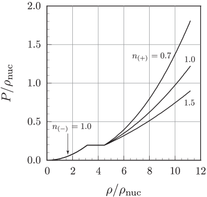
Now we have six parameters; the central density of the star ρcsubscript𝜌𝑐\rho_{c}, the inner density at the discontinuous surface ρdis(+)superscriptsubscript𝜌dis\rho_{\rm dis}^{(+)}, the ratio of the outer density to the inner density at the discontinuous surface ρdis()/ρdis(+)superscriptsubscript𝜌dissuperscriptsubscript𝜌dis\rho_{\rm dis}^{(-)}/\rho_{\rm dis}^{(+)}, the inner polytropic index n(+)subscript𝑛n_{(+)}, the outer polytropic index n()subscript𝑛n_{(-)} and the outer polytropic coefficient K()subscript𝐾K_{(-)}. Some examples of this equation of state with discontinuous density are given in Figure 1.
Refer to caption
FIG. 1.: Equation of state with density discontinuity. The density and pressure are normalized by the standard nuclear density ρnuc=2.68×10¹⁴subscript𝜌nuc2.68superscript1014\rho_{\rm nuc}=2.68\times 10^{14} (g/cm3). We set ρc=3.0×10¹⁵subscript𝜌𝑐3.0superscript1015\rho_{c}=3.0\times 10^{15} (g/cm3), ρdis(+)=1.2×10¹⁵superscriptsubscript𝜌dis1.2superscript1015\rho_{\rm dis}^{(+)}=1.2\times 10^{15} (g/cm3), ρdis()/ρdis(+)=0.7superscriptsubscript𝜌dissuperscriptsubscript𝜌dis0.7\rho_{\rm dis}^{(-)}/\rho_{\rm dis}^{(+)}=0.7, K()=100subscript𝐾100K_{(-)}=100 (km2) and n()=1.0subscript𝑛1.0n_{(-)}=1.0.

B perturbation equations inside the star

Here we present the basic equations for perturbations against the background metric of a spherically symmetric star (1). The perturbation is given by

gμν=gμν(B)+hμν.subscript𝑔𝜇𝜈subscriptsuperscript𝑔𝐵𝜇𝜈subscript𝜇𝜈g_{\mu\nu}=g^{(B)}_{\mu\nu}+h_{\mu\nu}. (10)

The perturbations against a spherical background can be decomposed by the spherical harmonics Ymlsubscriptsuperscript𝑌𝑙𝑚Y^{l}_{m}, and are classified into two by its parity, i.e. odd or even. Because we are interested in to discuss relation between a discontinuity in stellar density and the gravitational waves emitted from such a neutron star, in this paper, we only study even-parity perturbations, in which gravitational waves are coupled to fluid oscillation.

Following the method by Lindblom and Detweiler[12], hμνsubscript𝜇𝜈h_{\mu\nu} is described as

hμν=(rlH^e2Φiωrl+1H^100iωrl+1H^1rlH^e2Λ0000rl+2K^0000rl+2K^sin2θ)Ymleiωt,subscript𝜇𝜈superscript𝑟𝑙^𝐻superscript𝑒2Φ𝑖𝜔superscript𝑟𝑙1subscript^𝐻100𝑖𝜔superscript𝑟𝑙1subscript^𝐻1superscript𝑟𝑙^𝐻superscript𝑒2Λ0000superscript𝑟𝑙2^𝐾0000superscript𝑟𝑙2^𝐾superscript2𝜃subscriptsuperscript𝑌𝑙𝑚superscript𝑒𝑖𝜔𝑡h_{\mu\nu}=\left(\begin{array}[]{cccc}r^{l}\hat{H}e^{2\Phi}&i\omega r^{l+1}\hat{H}_{1}&0&0\\ i\omega r^{l+1}\hat{H}_{1}&r^{l}\hat{H}e^{2\Lambda}&0&0\\ 0&0&r^{l+2}\hat{K}&0\\ 0&0&0&r^{l+2}\hat{K}\sin^{2}\theta\end{array}\right)Y^{l}_{m}\,e^{i\omega t}, (11)

where H^,H^1,^𝐻subscript^𝐻1\hat{H},\hat{H}_{1}, and K^^𝐾\hat{K} are the perturbed metric function with respect to r𝑟r. The fluid perturbations are described by the Lagrangian displacement vectors ξi=(ξr,ξθ,ξϕ)superscript𝜉𝑖superscript𝜉𝑟superscript𝜉𝜃superscript𝜉italic-ϕ\xi^{i}=(\xi^{r},\xi^{\theta},\xi^{\phi}) as follows:

ξrsuperscript𝜉𝑟\displaystyle\xi^{r} =\displaystyle= rlreΛW^Ymleiωt,superscript𝑟𝑙𝑟superscript𝑒Λ^𝑊subscriptsuperscript𝑌𝑙𝑚superscript𝑒𝑖𝜔𝑡\displaystyle\frac{r^{l}}{r}e^{\Lambda}\hat{W}Y^{l}_{m}\,e^{i\omega t}, (12)
ξθsuperscript𝜉𝜃\displaystyle\xi^{\theta} =\displaystyle= rlr2eΛV^θYmleiωt,superscript𝑟𝑙superscript𝑟2superscript𝑒Λ^𝑉𝜃subscriptsuperscript𝑌𝑙𝑚superscript𝑒𝑖𝜔𝑡\displaystyle-\frac{r^{l}}{r^{2}}e^{\Lambda}\hat{V}\frac{\partial}{\partial\theta}Y^{l}_{m}\,e^{i\omega t}, (13)
ξϕsuperscript𝜉italic-ϕ\displaystyle\xi^{\phi} =\displaystyle= rlr2sin2θeΛV^ϕYmleiωt,superscript𝑟𝑙superscript𝑟2superscript2𝜃superscript𝑒Λ^𝑉italic-ϕsubscriptsuperscript𝑌𝑙𝑚superscript𝑒𝑖𝜔𝑡\displaystyle-\frac{r^{l}}{r^{2}\sin^{2}\theta}e^{\Lambda}\hat{V}\frac{\partial}{\partial\phi}Y^{l}_{m}\,e^{i\omega t}, (14)

where W^^𝑊\hat{W} and V^^𝑉\hat{V} are functions with respect to r𝑟r. Furthermore we introduce the new variable X^^𝑋\hat{X} instead of V^^𝑉\hat{V} to make the boundary condition at the surface of a star simple (see below);

X^ω2(P+ρ)eΦV^eΦΛrdPdrW^12(P+ρ)eΦH^.^𝑋superscript𝜔2𝑃𝜌superscript𝑒Φ^𝑉superscript𝑒ΦΛ𝑟𝑑𝑃𝑑𝑟^𝑊12𝑃𝜌superscript𝑒Φ^𝐻\hat{X}\equiv\omega^{2}\left(P+\rho\right)e^{-\Phi}\hat{V}-\frac{e^{\Phi-\Lambda}}{r}\frac{dP}{dr}\hat{W}-\frac{1}{2}\left(P+\rho\right)e^{\Phi}\hat{H}. (15)

The perturbation equations of the Einstein equations are given by

dH^1dr=1r[l+1+2mre2Λ+4πr2(Pρ)e2Λ]H^1𝑑subscript^𝐻1𝑑𝑟1𝑟delimited-[]𝑙12𝑚𝑟superscript𝑒2Λ4𝜋superscript𝑟2𝑃𝜌superscript𝑒2Λsubscript^𝐻1\displaystyle\frac{d\hat{H}_{1}}{dr}=-\frac{1}{r}\left[l+1+\frac{2m}{r}e^{2\Lambda}+4\pi r^{2}(P-\rho)e^{2\Lambda}\right]\hat{H}_{1} (16)
+1re2Λ[H^+K^+16π(P+ρ)V^],1𝑟superscript𝑒2Λdelimited-[]^𝐻^𝐾16𝜋𝑃𝜌^𝑉\displaystyle\hskip 34.14322pt+\frac{1}{r}e^{2\Lambda}\left[\hat{H}+\hat{K}+16\pi(P+\rho)\hat{V}\right], (17)
dK^dr=l(l+1)2rH^1+1rH^(l+1rdΦdr)K^+8πr(P+ρ)eΛW^,𝑑^𝐾𝑑𝑟𝑙𝑙12𝑟subscript^𝐻11𝑟^𝐻𝑙1𝑟𝑑Φ𝑑𝑟^𝐾8𝜋𝑟𝑃𝜌superscript𝑒Λ^𝑊\displaystyle\frac{d\hat{K}}{dr}=\frac{l(l+1)}{2r}\hat{H}_{1}+\frac{1}{r}\hat{H}-\left(\frac{l+1}{r}-\frac{d\Phi}{dr}\right)\hat{K}+\frac{8\pi}{r}(P+\rho)e^{\Lambda}\hat{W}, (18)
dW^dr=l+1rW^+reΛ[1γPeΦX^l(l+1)r2V^12H^K^],𝑑^𝑊𝑑𝑟𝑙1𝑟^𝑊𝑟superscript𝑒Λdelimited-[]1𝛾𝑃superscript𝑒Φ^𝑋𝑙𝑙1superscript𝑟2^𝑉12^𝐻^𝐾\displaystyle\frac{d\hat{W}}{dr}=-\frac{l+1}{r}\hat{W}+re^{\Lambda}\left[\frac{1}{\gamma P}e^{-\Phi}\hat{X}-\frac{l(l+1)}{r^{2}}\hat{V}-\frac{1}{2}\hat{H}-\hat{K}\right], (19)
dX^dr=lrX^+(P+ρ)eΦ[12(dΦdr1r)H^12(ω2re2Φ+l(l+1)2r)H^1\displaystyle\frac{d\hat{X}}{dr}=-\frac{l}{r}\hat{X}+(P+\rho)e^{\Phi}\biggl{[}\frac{1}{2}\left(\frac{d\Phi}{dr}-\frac{1}{r}\right)\hat{H}-\frac{1}{2}\left(\omega^{2}re^{-2\Phi}+\frac{l(l+1)}{2r}\right)\hat{H}_{1} (20)
+(12r32dΦdr)K^l(l+1)r2dΦdrV^12𝑟32𝑑Φ𝑑𝑟^𝐾𝑙𝑙1superscript𝑟2𝑑Φ𝑑𝑟^𝑉\displaystyle\hskip 34.14322pt+\left(\frac{1}{2r}-\frac{3}{2}\frac{d\Phi}{dr}\right)\hat{K}-\frac{l(l+1)}{r^{2}}\frac{d\Phi}{dr}\hat{V} (21)
1r(ω2e2Φ+Λ+4π(P+ρ)eΛr2{ddr(1r2eΛdΦdr)})W^],\displaystyle\hskip 34.14322pt-\frac{1}{r}\left(\omega^{2}e^{-2\Phi+\Lambda}+4\pi(P+\rho)e^{\Lambda}-r^{2}\left\{\frac{d}{dr}\left(\frac{1}{r^{2}}e^{-\Lambda}\frac{d\Phi}{dr}\right)\right\}\right)\hat{W}\biggr{]}, (22)
[13mrl(l+1)24πr2P]H^8πr2eΦX^delimited-[]13𝑚𝑟𝑙𝑙124𝜋superscript𝑟2𝑃^𝐻8𝜋superscript𝑟2superscript𝑒Φ^𝑋\displaystyle\biggl{[}1-\frac{3m}{r}-\frac{l(l+1)}{2}-4\pi r^{2}P\biggr{]}\hat{H}-8\pi r^{2}e^{-\Phi}\hat{X} (23)
+r2e2Λ[ω2e2Φl(l+1)2rdΦdr]H^1superscript𝑟2superscript𝑒2Λdelimited-[]superscript𝜔2superscript𝑒2Φ𝑙𝑙12𝑟𝑑Φ𝑑𝑟subscript^𝐻1\displaystyle\hskip 34.14322pt+r^{2}e^{-2\Lambda}\left[\omega^{2}e^{-2\Phi}-\frac{l(l+1)}{2r}\frac{d\Phi}{dr}\right]\hat{H}_{1} (24)
[1+ω2r2e2Φl(l+1)2(r3m4πr3P)dΦdr]K^=0,delimited-[]1superscript𝜔2superscript𝑟2superscript𝑒2Φ𝑙𝑙12𝑟3𝑚4𝜋superscript𝑟3𝑃𝑑Φ𝑑𝑟^𝐾0\displaystyle\hskip 34.14322pt-\left[1+\omega^{2}r^{2}e^{-2\Phi}-\frac{l(l+1)}{2}-\left(r-3m-4\pi r^{3}P\right)\frac{d\Phi}{dr}\right]\hat{K}=0, (25)
V^=e2Φω2(P+ρ)[eΦX^+1rdPdreΛW^+12(P+ρ)H^],^𝑉superscript𝑒2Φsuperscript𝜔2𝑃𝜌delimited-[]superscript𝑒Φ^𝑋1𝑟𝑑𝑃𝑑𝑟superscript𝑒Λ^𝑊12𝑃𝜌^𝐻\displaystyle\hat{V}=\frac{e^{2\Phi}}{\omega^{2}(P+\rho)}\left[e^{-\Phi}\hat{X}+\frac{1}{r}\frac{dP}{dr}e^{-\Lambda}\hat{W}+\frac{1}{2}(P+\rho)\hat{H}\right], (26)

where γ𝛾\gamma is the adiabatic index of the unperturbed stellar model defined by

γ=ρ+PP(Pρ)ad.𝛾𝜌𝑃𝑃subscript𝑃𝜌ad\gamma=\frac{\rho+P}{P}\left(\frac{\partial P}{\partial\rho}\right)_{\rm ad}. (27)

Eqs. (17)-(22) give a set of differential equations for the variables H^1subscript^𝐻1\hat{H}_{1}, K^^𝐾\hat{K}, W^^𝑊\hat{W} and X^^𝑋\hat{X}, while Eqs. (25) and (26) are the algebraic equations for the variables H^^𝐻\hat{H} and V^^𝑉\hat{V}.

C the perturbations outside the stars

In the region outside the star, the perturbations are described by the Zerilli equations. Setting m=M,W^=V^=0formulae-sequence𝑚𝑀^𝑊^𝑉0m=M,\hat{W}=\hat{V}=0, and replacing H^1,K^subscript^𝐻1^𝐾\hat{H}_{1},\hat{K} with new variables Z𝑍Z, dZ/dr𝑑𝑍𝑑subscript𝑟dZ/dr_{*} defined by

rlK^superscript𝑟𝑙^𝐾\displaystyle r^{l}\hat{K} =\displaystyle= λ(λ+1)r2+3λMr+6M2r2(λr+3M)Z+dZdr,𝜆𝜆1superscript𝑟23𝜆𝑀𝑟6superscript𝑀2superscript𝑟2𝜆𝑟3𝑀𝑍𝑑𝑍𝑑subscript𝑟\displaystyle\frac{\lambda(\lambda+1)r^{2}+3\lambda Mr+6M^{2}}{r^{2}(\lambda r+3M)}Z+\frac{dZ}{dr_{*}}, (28)
rl+1H^1superscript𝑟𝑙1subscript^𝐻1\displaystyle r^{l+1}\hat{H}_{1} =\displaystyle= λr23λMr3M2(r2M)(λr+3M)Z+r2r2MdZdr,𝜆superscript𝑟23𝜆𝑀𝑟3superscript𝑀2𝑟2𝑀𝜆𝑟3𝑀𝑍superscript𝑟2𝑟2𝑀𝑑𝑍𝑑subscript𝑟\displaystyle\frac{\lambda r^{2}-3\lambda Mr-3M^{2}}{(r-2M)(\lambda r+3M)}Z+\frac{r^{2}}{r-2M}\frac{dZ}{dr_{*}}, (29)

we recover the Zerilli equations. Here rsubscript𝑟r_{*} is the tortoise coordinates and λl(l+1)/21𝜆𝑙𝑙121\lambda\equiv l(l+1)/2-1.

D boundary conditions

In order to solve the above perturbation equations, we have to impose the boundary conditions. At the center of the star, we have regularity condition for the perturbative variables. We expand all variables by Taylor power-series near r=0𝑟0r=0 in a similar way of Detweiler and Lindblom [12] (see Appendix A). Another boundary condition is that the pressure vanishes at the stellar surface. Then the perturbed pressure X^^𝑋\hat{X}, ΔPΔ𝑃\Delta P is given by

ΔP=rleΦX^Δ𝑃superscript𝑟𝑙superscript𝑒Φ^𝑋\Delta P=-r^{l}e^{-\Phi}\hat{X} (30)

also vanishes there. This boundary condition at the surface of star is equivalent to X^(R)=0^𝑋𝑅0\hat{X}(R)=0. The last condition is that there exist only outgoing gravitational waves at infinity. We also have a junction condition at the surface of discontinuity, where the variables of H^1,K^,W^,ΔPsubscript^𝐻1^𝐾^𝑊Δ𝑃\hat{H}_{1},\hat{K},\hat{W},\Delta P (and then X^^𝑋\hat{X}) must be continuous. Note that, H^^𝐻\hat{H} and V^^𝑉\hat{V} are determined by Eqs. (25) and (26). H^^𝐻\hat{H} is continuos but V^^𝑉\hat{V} is discontinuous.

III numerical results

A models of neutron star

As a concrete example of density discontinuity, we know kaon condensation [2], which may occur at ρdis(+)=1.466×10¹⁵superscriptsubscript𝜌dis1.466superscript1015\rho_{\rm dis}^{(+)}=1.466\times 10^{15} g/cm3 with the discontinuity ρdis()/ρdis(+)=0.414superscriptsubscript𝜌dissuperscriptsubscript𝜌dis0.414\rho_{\rm dis}^{(-)}/\rho_{\rm dis}^{(+)}=0.414 for a cold neutron star. Hence we consider density discontinuity around this value, i.e. we study the following three cases: ρdis(+)=8.0×10¹⁴superscriptsubscript𝜌dis8.0superscript1014\rho_{\rm dis}^{(+)}=8.0\times 10^{14}, 1.2×10151.2superscript10151.2\times 10^{15} and 1.6×10151.6superscript10151.6\times 10^{15} g/cm3. First we briefly discuss a models of a neutron star with density discontinuity. As mentioned before, we have six unknown parameters: n(),K(),n(+),ρdis(+),ρdis()/ρdis(+)subscript𝑛subscript𝐾subscript𝑛superscriptsubscript𝜌dissuperscriptsubscript𝜌dissuperscriptsubscript𝜌disn_{(-)},K_{(-)},n_{(+)},\rho_{\rm dis}^{(+)},\rho_{\rm dis}^{(-)}/\rho_{\rm dis}^{(+)} and ρcsubscript𝜌𝑐\rho_{c}. We set n()=1.0subscript𝑛1.0n_{(-)}=1.0 and K()=100(km2)subscript𝐾100superscriptkm2K_{(-)}=100\,(\text{km}^{2}), which are usually adopted in a neutron star model. The rest four are n(+),ρdis(+),ρdis()/ρdis(+)subscript𝑛superscriptsubscript𝜌dissuperscriptsubscript𝜌dissuperscriptsubscript𝜌disn_{(+)},\rho_{\rm dis}^{(+)},\rho_{\rm dis}^{(-)}/\rho_{\rm dis}^{(+)} and ρcsubscript𝜌𝑐\rho_{c}.

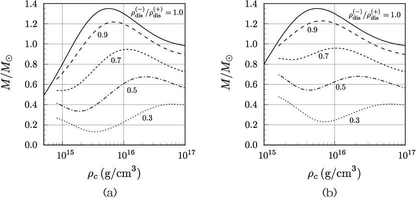
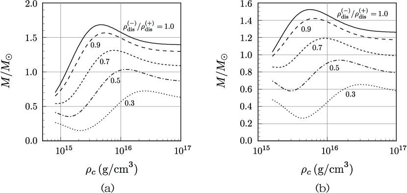
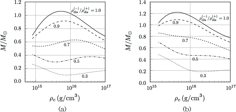
First we show the gravitational mass M𝑀M with respect to a central density ρcsubscript𝜌𝑐\rho_{c} for several values of n(+),ρdis(+),ρdis()/ρdis(+)subscript𝑛superscriptsubscript𝜌dissuperscriptsubscript𝜌dissuperscriptsubscript𝜌disn_{(+)},\rho_{\rm dis}^{(+)},\rho_{\rm dis}^{(-)}/\rho_{\rm dis}^{(+)} in Figs. 2-4.

Refer to caption
FIG. 2.: The relation between the central density ρcsubscript𝜌𝑐\rho_{c} and the gravitational mass of a neutron star M𝑀M for n(+)=1.0subscript𝑛1.0n_{(+)}=1.0. Fig. 2(a) is the case of ρdis(+)=8.0×10¹⁴superscriptsubscript𝜌dis8.0superscript1014\rho_{\rm dis}^{(+)}=8.0\times 10^{14}  (g/cm3) , while Fig. 2(b) is the case of ρdis(+)=1.6×10¹⁵superscriptsubscript𝜌dis1.6superscript1015\rho_{\rm dis}^{(+)}=1.6\times 10^{15}  (g/cm3). The numbers associated with each curve are the values of ρdis()/ρdis(+)superscriptsubscript𝜌dissuperscriptsubscript𝜌dis\rho_{\rm dis}^{(-)}/\rho_{\rm dis}^{(+)}.
Refer to caption
FIG. 3.: The same figures as Fig. 2 for the case of n(+)=0.7subscript𝑛0.7n_{(+)}=0.7.

As for inner polytropic index, we set n(+)=subscript𝑛absentn_{(+)}= 1.0 (Fig. 2), 0.7 (Fig. 3), 1.5 (Fig. 4). For each polytropic index, we consider two models with different density at discontinuity:ρdis(+)=8.0×10¹⁴superscriptsubscript𝜌dis8.0superscript1014\rho_{\rm dis}^{(+)}=8.0\times 10^{14} (a) and 1.6×10151.6superscript10151.6\times 10^{15} g/cm3 (b). We depict the M𝑀M-ρcsubscript𝜌𝑐\rho_{c} diagram for each value of ρdis()/ρdis(+)superscriptsubscript𝜌dissuperscriptsubscript𝜌dis\rho_{\rm dis}^{(-)}/\rho_{\rm dis}^{(+)} = 1.0 (no discontinuity), 0.9, 0.7, 0.5, and 0.3. Fig. 2 for n(+)=1.0subscript𝑛1.0n_{(+)}=1.0 shows that the maximum masses for each value of ρdis()/ρdis(+)superscriptsubscript𝜌dissuperscriptsubscript𝜌dis\rho_{\rm dis}^{(-)}/\rho_{\rm dis}^{(+)} do not depend on density discontinuity ρdis(+)superscriptsubscript𝜌dis\rho_{\rm dis}^{(+)}. As ρdis()/ρdis(+)superscriptsubscript𝜌dissuperscriptsubscript𝜌dis\rho_{\rm dis}^{(-)}/\rho_{\rm dis}^{(+)} gets small, the maximum mass decreases and the stable region (dM/dρc>0𝑑𝑀𝑑subscript𝜌𝑐0dM/d\rho_{c}>0) becomes narrower and moves to high density region.

For n(+)1.0subscript𝑛1.0n_{(+)}\neq 1.0, the maximum mass depends on ρdis(+)superscriptsubscript𝜌dis\rho_{\rm dis}^{(+)}. In fact, for n(+)<1.0subscript𝑛1.0n_{(+)}<1.0 (Fig. 3), the maximum mass decreases as ρdis(+)superscriptsubscript𝜌dis\rho_{\rm dis}^{(+)} increases, while for n(+)>1.0subscript𝑛1.0n_{(+)}>1.0 (Fig. 4), the maximum mass increases. As the equation of state of inner region becomes more stiff, i.e. as n(+)subscript𝑛n_{(+)} decreases, the maximum mass gets large. The other properties about maximum mass for n(+)=0.7subscript𝑛0.7n_{(+)}=0.7 and 1.51.51.5 are same as those of n(+)=1.0subscript𝑛1.0n_{(+)}=1.0. Note that for the case of n(+)=1.5subscript𝑛1.5n_{(+)}=1.5, all stellar models are unstable if discontinuity gets large.

In what follows, we discuss only stable stellar models, i.e. dM/dρc>0𝑑𝑀𝑑subscript𝜌𝑐0dM/d\rho_{c}>0. In our analysis, we fix the mass of a neutron star M𝑀M (1.2M1.2subscript𝑀direct-product1.2M_{\odot}, 0.5M0.5subscript𝑀direct-product0.5M_{\odot}) because M𝑀M may be determined by other observations. In Table I, Table II and Table III, we summarize the properties of background stellar models.
Refer to caption
FIG. 4.: The same figures as Fig. 2 for the case of n(+)=1.5subscript𝑛1.5n_{(+)}=1.5.

B Quasi-normal modes for a stellar model without discontinuity

In order to find a specific property in quasi-normal modes of a neutron star with discontinuity, first we calculate of l=2𝑙2l=2 in the case of a stellar model without discontinuity as reference. In this case, we have to set two parameters; the polytropic index n𝑛n and polytropic coefficient K𝐾K, if we fix the total mass M𝑀M. We adopt the following values; (n,K)=(1.0,100km2)𝑛𝐾1.0100superscriptkm2(n,K)=(1.0,100\text{km}^{2}), (1.0,200km2)1.0200superscriptkm2(1.0,200\text{km}^{2}), (1.5,15km4/3)1.515superscriptkm43(1.5,15\text{km}^{4/3}), (2.0,3.5km)2.03.5km(2.0,3.5\text{km}) for M=1.2M𝑀1.2subscript𝑀direct-productM=1.2M_{\odot}. We also the case of M=0.5M𝑀0.5subscript𝑀direct-productM=0.5M_{\odot} with (n,K)=(1.0,100km2)𝑛𝐾1.0100superscriptkm2(n,K)=(1.0,100\text{km}^{2}) to examine the mass dependence. The properties of the neutron star models are summarized in Table IV.

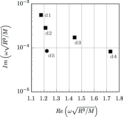
The quasi-normal modes of the gravitational wave emitted from such stars are plotted in Figure 5 and listed in Table V. The plot point corresponds to the so-called f-mode of each stellar model. In this table we show the mode frequency ω𝜔\omega by two normalizations: one is ωM𝜔𝑀\omega M and the other is ω(R3/M)1/2𝜔superscriptsuperscript𝑅3𝑀12\omega(R^{3}/M)^{1/2}. Although the f-mode is determined by the radius as well as the mass, we may not know the radius from observation. Then we can plot the data by ωM𝜔𝑀\omega M. In the figure, however, we only show  ω(R3/M)1/2𝜔superscriptsuperscript𝑅3𝑀12\omega(R^{3}/M)^{1/2}. In a neutron star, we usually find many p-modes as well as f-mode, but we only show the lowest f-mode here because that we are interested in new mode which appears in low frequency for a star with discontinuity.
Refer to caption
FIG. 5.: The quasi normal mode (f-mode) of a neutron star without density discontinuity. The labels associated with each mark correspond to the models in Table IV.

From Fig. 5, we find that the real part of eigenfrequency gets large as equation of state is softer. For example, the frequency in the case ’d4’ is by 47%percent4747\% larger than that in the case ’d1’. However, this tendency becomes reverse if we use another normalization (ωM𝜔𝑀\omega M) because the radius of a neutron star constructed by soft matter is larger than one constructed by stiff matter (see Table IV). We also find that the imaginary part of eigenfrequency increases as the stellar mass increases, but the real part is insensitive to the mass.

C Quasi-normal modes for a stellar model with discontinuity

In the case with discontinuity, we have three unknown parameters: n(+)subscript𝑛n_{(+)}, ρdis(+)superscriptsubscript𝜌dis\rho_{\rm dis}^{(+)} and ρdis()/ρdis(+)superscriptsubscript𝜌dissuperscriptsubscript𝜌dis\rho_{\rm dis}^{(-)}/\rho_{\rm dis}^{(+)}. First we show the eigenfrequency of quasi-normal modes of l=2𝑙2l=2 for the case of n(+)=1.0subscript𝑛1.0n_{(+)}=1.0. We fix the mass of a neutron star as M=1.2M𝑀1.2subscript𝑀direct-productM=1.2M_{\odot} or 0.5M0.5subscript𝑀direct-product0.5M_{\odot}. Now two free parameters are ρdis(+)superscriptsubscript𝜌dis\rho_{\rm dis}^{(+)} and ρdis()/ρdis(+)superscriptsubscript𝜌dissuperscriptsubscript𝜌dis\rho_{\rm dis}^{(-)}/\rho_{\rm dis}^{(+)}.

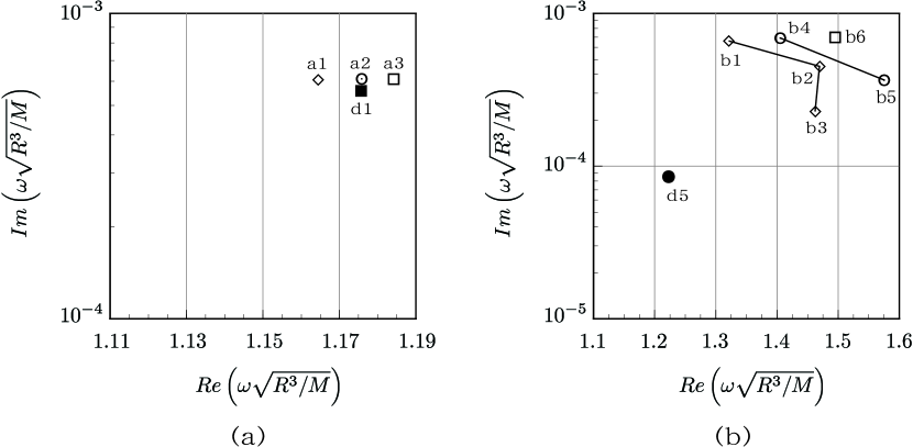
We show the f-mode for M=1.2M𝑀1.2subscript𝑀direct-productM=1.2M_{\odot} and 0.5M0.5subscript𝑀direct-product0.5M_{\odot} in Fig. 6. The numerical values are given in Table VI and Table VII.

Refer to caption
FIG. 6.: The quasi normal mode (f-mode) of a neutron star with density discontinuity. We set n(+)=1.0subscript𝑛1.0n_{(+)}=1.0. The left figure (a) shows the result of a star with M=1.2M𝑀1.2subscript𝑀direct-productM=1.2M_{\odot}, while the right one (b) corresponds to a star with M=0.5M𝑀0.5subscript𝑀direct-productM=0.5M_{\odot}. The labels associated with each mark correspond to the models in Table I and in Table II. The data of ’d1’ and ’d5’, which are the models without discontinuity for n=1.0𝑛1.0n=1.0 and K=100𝐾100K=100 (km2), are also plotted as a reference.

For f-mode, we find that the mode frequency for less massive star (0.5 Msubscript𝑀direct-productM_{\odot}) is more sensitive to discontinuity than that for massive star (1.2 Msubscript𝑀direct-productM_{\odot}). For example, the difference of the model ’b5’ from the model without discontinuity is larger than 28% for 0.5M0.5subscript𝑀direct-product0.5M_{\odot}. It is also found that the imaginary part of eigenfrequencies in the model with discontinuity is larger than one without discontinuity, and this difference becomes larger as M/R𝑀𝑅M/R increases.

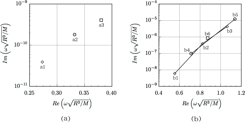
The results of g-mode for M=1.2M𝑀1.2subscript𝑀direct-productM=1.2M_{\odot} and 0.5M0.5subscript𝑀direct-product0.5M_{\odot} are given in Fig. 7 and in Table VIII and Table IX. For g-mode, we also find the similar properties to the f-mode. The mode frequency in a less massive star is more sensitive than that in a massive star, in particular the imaginary part changes by the factor 102104superscript102superscript10410^{2}-10^{4} for the same ρdis(+)superscriptsubscript𝜌dis\rho_{\rm dis}^{(+)} depending on the amount of discontinuity (see Fig.7). Furthermore, the existence of g-mode is due to discontinuity, and it turns out that its imaginary part of g-mode is not always so small if the discontinuity is very large. We conclude that the damping rate of g-mode may not be ignored in a particular situation.

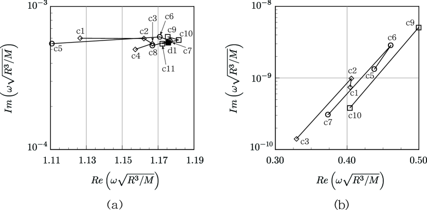
Next we calculate the eigenfrequencies of f-mode and g-mode for n(+)=0.7subscript𝑛0.7n_{(+)}=0.7. The results of f-modes and g-mode are shown in Fig. 8(a) with the case of the model without discontinuity, and in Fig. 8(b), respectively. The numerical data are given in Table X and Table XI, respectively. By comparing the upper panel in Fig. 6(a), we find that the effect of change of equation of state is quite small. On the other hand, the imaginary part of g-mode becomes by 10 times larger than the case of n=1𝑛1n=1 due to the existence of the inner stiff matter. Furthermore, in this case, even if the density is continuous (ρdis()/ρdis(+)=1.0superscriptsubscript𝜌dissuperscriptsubscript𝜌dis1.0\rho_{\rm dis}^{(-)}/\rho_{\rm dis}^{(+)}=1.0), one may expect the appearance of g-mode because of discontinuity of the equation of state (n(+)=0.7subscript𝑛0.7n_{(+)}=0.7 and n()=1.0subscript𝑛1.0n_{(-)}=1.0). However, we could not find g-mode in our calculation. This may be because the g-mode does not exist or is too small to be found.
Refer to caption
FIG. 7.: The quasi normal mode (g-mode) of a neutron star with density discontinuity. The setting is the same as Fig. 6.
Refer to caption
FIG. 8.: The quasi normal modes of a neutron star with density discontinuity ((a) f-mode and (b) g-mode). We set n(+)=0.7subscript𝑛0.7n_{(+)}=0.7 and M=1.2M𝑀1.2subscript𝑀direct-productM=1.2M_{\odot}. The labels associated with each mark correspond to the models in Table III. The data of ’d1’, which is the model without discontinuity for n=1.0𝑛1.0n=1.0 and K=100𝐾100K=100 (km2), are also plotted as a reference.

D Comparison with the Cowling approximation

Finally, by using relativistic Cowling approximation [11], we shall calculate the f- and g-modes, and compare them to our results. In the Cowling approximation, metric perturbation is ignored and only stellar oscillation is taken into account. Hence, the eigenfrequency has only the real part. The result is given in Table XII for ρ(+)=8.0×10¹⁴subscript𝜌8.0superscript1014\rho_{(+)}=8.0\times 10^{14} (g/cm3). The error (the difference from our numerical value) estimated by

error=ωCowe(ω)e(ω),𝑒𝑟𝑟𝑜𝑟subscript𝜔Cow𝑒𝜔𝑒𝜔error=\frac{\omega_{\rm Cow}-{\cal R}e(\omega)}{{\cal R}e(\omega)}, (31)

is also shown. Here ωCowsubscript𝜔Cow\omega_{\rm Cow} is the eigenfrequency found by the Cowling approximation, and ωCow(g)superscriptsubscript𝜔Cow𝑔\omega_{\rm Cow}^{(g)} and ωCow(f)superscriptsubscript𝜔Cow𝑓\omega_{\rm Cow}^{(f)} denote those of g- and f-modes, respectively. From Table XII, we find that the Cowling approximation is very accurate for g-mode if ρ(+)subscript𝜌\rho_{(+)} is at least in this region, although it is not so good for the f-mode.

IV conclusion

In this paper we calculate the eigenfrequencies of f-mode and g-mode to examine the dependence of the discontinuity of the density if there exists. We investigate with the various discontinuity, by changing ρdis(+)superscriptsubscript𝜌dis\rho_{\rm dis}^{(+)} and ρdis()/ρdis(+)superscriptsubscript𝜌dissuperscriptsubscript𝜌dis\rho_{\rm dis}^{(-)}/\rho_{\rm dis}^{(+)}, for the case that the total mass is fixed 1.2M1.2subscript𝑀direct-product1.2M_{\odot} for n(+)=1.0subscript𝑛1.0n_{(+)}=1.0, 0.70.70.7 and 0.5M0.5subscript𝑀direct-product0.5M_{\odot} for n(+)=1.0subscript𝑛1.0n_{(+)}=1.0. In consequence we find that the dependence of the eigenfrequencies of f-mode on the discontinuity of the density is more strongly for the case that the total mass is smaller. The effect that the inner matter is stiff, n(+)=0.7subscript𝑛0.7n_{(+)}=0.7 and n()=1.0subscript𝑛1.0n_{(-)}=1.0, is quite small for f-mode. And it is found that the imaginary part of the eigenfrequencies of g-mode become a little large for the case that inner matter is stiff. In general imaginary part of g-mode is quite small, but we find that in particular situation such that an inner polytropic index is the same as an outer one and total mass is rather small, the imaginary part of g-mode may not be ignored.

For the considering the circumstances mentioned above, it might be possible to judge whether the discontinuity of the density exist or not by the direct observation of the gravitational waves, which might be practicable in future observation, for even f-mode in the particular situation which the total mass is small. Of course, if the gravitational waves of g-mode is directly observed for such stars as the small massive ones, it is found that the discontinuity of the density exist. So we can judge the existence of the phase transition of the density in the neutron stars by the direct observation of the gravitational waves, though we need to collect the detailed data of the eigenfrequencies for some characteristic mode.

Finally we find also that Cowling approximation is quite accurate for g-mode.

Acknowledgements.
We would like to thank M. Saijo for useful discussion. HS acknowledges T. Harada for valuable comments. This work was supported partially by JSPS Grants-in-Aid (No. 1205705) and by the Waseda University Grant for Special Research Projects.

A the Taylor expansion at the center of a neutron star

Here we present the explicit perturbation equations (17)- (26) by the expansion at the center of a neutron star. ρ𝜌\rho, P𝑃P and ΦΦ\Phi are expanded at r=0𝑟0r=0 as

ρ(r)𝜌𝑟\displaystyle\rho(r) =\displaystyle= ρ(0)+12ρ(2)r2+O(r4),superscript𝜌012superscript𝜌2superscript𝑟2𝑂superscript𝑟4\displaystyle\rho^{(0)}+\frac{1}{2}\rho^{(2)}r^{2}+O(r^{4}), (A1)
P(r)𝑃𝑟\displaystyle P(r) =\displaystyle= P(0)+12P(2)r2+14P(4)r4+O(r6),superscript𝑃012superscript𝑃2superscript𝑟214superscript𝑃4superscript𝑟4𝑂superscript𝑟6\displaystyle P^{(0)}+\frac{1}{2}P^{(2)}r^{2}+\frac{1}{4}P^{(4)}r^{4}+O(r^{6}), (A2)
Φ(r)Φ𝑟\displaystyle\Phi(r) =\displaystyle= Φ(0)+12Φ(2)r2+14Φ(4)r4+O(r6).superscriptΦ012superscriptΦ2superscript𝑟214superscriptΦ4superscript𝑟4𝑂superscript𝑟6\displaystyle\Phi^{(0)}+\frac{1}{2}\Phi^{(2)}r^{2}+\frac{1}{4}\Phi^{(4)}r^{4}+O(r^{6}). (A3)

where the coefficients are obtained from Eqs. (2)-(4) and (27) as

Φ(2)superscriptΦ2\displaystyle\Phi^{(2)} =4π3ρ(0)+4πP(0),absent4𝜋3superscript𝜌04𝜋superscript𝑃0\displaystyle=\frac{4\pi}{3}\rho^{(0)}+4\pi P^{(0)}, (A4)
P(2)superscript𝑃2\displaystyle P^{(2)} =(P(0)+ρ(0))Φ(2),absentsuperscript𝑃0superscript𝜌0superscriptΦ2\displaystyle=-\left(P^{(0)}+\rho^{(0)}\right)\Phi^{(2)}, (A5)
ρ(2)superscript𝜌2\displaystyle\rho^{(2)} =P(0)+ρ(0)P(0)γ(0)P(2),absentsuperscript𝑃0superscript𝜌0superscript𝑃0superscript𝛾0superscript𝑃2\displaystyle=\frac{P^{(0)}+\rho^{(0)}}{P^{(0)}\gamma^{(0)}}P^{(2)}, (A6)
Φ(4)superscriptΦ4\displaystyle\Phi^{(4)} =2π5ρ(2)+2πP(2)+32π29ρ(0)2+32π23ρ(0)P(0),absent2𝜋5superscript𝜌22𝜋superscript𝑃232superscript𝜋29superscriptsuperscript𝜌0232superscript𝜋23superscript𝜌0superscript𝑃0\displaystyle=\frac{2\pi}{5}\rho^{(2)}+2\pi P^{(2)}+\frac{32\pi^{2}}{9}{\rho^{(0)}}^{2}+\frac{32\pi^{2}}{3}\rho^{(0)}P^{(0)}, (A7)
P(4)superscript𝑃4\displaystyle P^{(4)} =(P(0)+ρ(0))Φ(4)12(P(2)+ρ(2))Φ(2).absentsuperscript𝑃0superscript𝜌0superscriptΦ412superscript𝑃2superscript𝜌2superscriptΦ2\displaystyle=-\left(P^{(0)}+\rho^{(0)}\right)\Phi^{(4)}-\frac{1}{2}\left(P^{(2)}+\rho^{(2)}\right)\Phi^{(2)}. (A8)

γ(0)superscript𝛾0\gamma^{(0)} is the adiabatic index at r=0𝑟0r=0, which is defined by the equation of state. The perturbation variables H^1subscript^𝐻1\hat{H}_{1}, K^^𝐾\hat{K}, W^^𝑊\hat{W} and X^^𝑋\hat{X} are expanded at r=0𝑟0r=0 follows,

H^1(r)subscript^𝐻1𝑟\displaystyle\hat{H}_{1}(r) =H^1(0)+12H^1(2)r2+O(r4),absentsuperscriptsubscript^𝐻1012superscriptsubscript^𝐻12superscript𝑟2𝑂superscript𝑟4\displaystyle={\hat{H}_{1}}^{(0)}+\frac{1}{2}{\hat{H}_{1}}^{(2)}r^{2}+O(r^{4}), (A9)
K^(r)^𝐾𝑟\displaystyle\hat{K}(r) =K^(0)+12K^(2)r2+O(r4),absentsuperscript^𝐾012superscript^𝐾2superscript𝑟2𝑂superscript𝑟4\displaystyle=\hat{K}^{(0)}+\frac{1}{2}\hat{K}^{(2)}r^{2}+O(r^{4}), (A10)
W^(r)^𝑊𝑟\displaystyle\hat{W}(r) =W^(0)+12W^(2)r2+O(r4),absentsuperscript^𝑊012superscript^𝑊2superscript𝑟2𝑂superscript𝑟4\displaystyle=\hat{W}^{(0)}+\frac{1}{2}\hat{W}^{(2)}r^{2}+O(r^{4}), (A11)
X^(r)^𝑋𝑟\displaystyle\hat{X}(r) =X^(0)+12X^(2)r2+O(r4),absentsuperscript^𝑋012superscript^𝑋2superscript𝑟2𝑂superscript𝑟4\displaystyle=\hat{X}^{(0)}+\frac{1}{2}\hat{X}^{(2)}r^{2}+O(r^{4}), (A12)

where the leading order coefficients in these equations are fixed by the perturbation equations (17)-(26) as

H^(0)1subscriptsuperscript^𝐻01\displaystyle{\hat{H}^{(0)}}_{1} =1l(l+1)[2lK^(0)16π(P(0)+ρ(0))W^(0)],absent1𝑙𝑙1delimited-[]2𝑙superscript^𝐾016𝜋superscript𝑃0superscript𝜌0superscript^𝑊0\displaystyle=\frac{1}{l(l+1)}\left[2l{\hat{K}^{(0)}}-16\pi\left({P^{(0)}}+{\rho^{(0)}}\right){\hat{W}^{(0)}}\right], (A13)
X^(0)superscript^𝑋0\displaystyle{\hat{X}^{(0)}} =(P(0)+ρ(0))eΦ(0)[12K^(0)+(4π3ρ(0)+4πP(0)ω2le2Φ(0))W^(0)].absentsuperscript𝑃0superscript𝜌0superscript𝑒superscriptΦ0delimited-[]12superscript^𝐾04𝜋3superscript𝜌04𝜋superscript𝑃0superscript𝜔2𝑙superscript𝑒2superscriptΦ0superscript^𝑊0\displaystyle=({P^{(0)}}+{\rho^{(0)}})e^{{\Phi^{(0)}}}\left[-\frac{1}{2}{\hat{K}^{(0)}}+\left(\frac{4\pi}{3}\rho^{(0)}+4\pi P^{(0)}-\frac{\omega^{2}}{l}e^{-2{\Phi^{(0)}}}\right){\hat{W}^{(0)}}\right]. (A14)

In the similar way, by using the equations (17)- (26), we find the second order coefficients in the expansion as

l+32H1^(2)K^(2)+8π(P(0)+ρ(0))l+3l(l+1)W^(2)𝑙32superscript^subscript𝐻12superscript^𝐾28𝜋superscript𝑃0superscript𝜌0𝑙3𝑙𝑙1superscript^𝑊2\displaystyle\frac{l+3}{2}\hat{H_{1}}^{(2)}-\hat{K}^{(2)}+8\pi(P^{(0)}+\rho^{(0)})\frac{l+3}{l(l+1)}\hat{W}^{(2)} (A15)
={4π3(2l+3)4πP(0)}H1^(0)8πl(P(2)+ρ(2))W^(0)+8π(P(0)+ρ(0))Q1+12Q0,absent4𝜋32𝑙34𝜋superscript𝑃0superscript^subscript𝐻108𝜋𝑙superscript𝑃2superscript𝜌2superscript^𝑊08𝜋superscript𝑃0superscript𝜌0subscript𝑄112subscript𝑄0\displaystyle\hskip 28.45274pt=\left\{\frac{4\pi}{3}(2l+3)-4\pi P^{(0)}\right\}\hat{H_{1}}^{(0)}-\frac{8\pi}{l}(P^{(2)}+\rho^{(2)})\hat{W}^{(0)}+8\pi(P^{(0)}+\rho^{(0)})Q_{1}+\frac{1}{2}Q_{0}, (A16)
l+22K^(2)l(l+1)4H1^(2)4π(P(0)+ρ(0))W^(2)𝑙22superscript^𝐾2𝑙𝑙14superscript^subscript𝐻124𝜋superscript𝑃0superscript𝜌0superscript^𝑊2\displaystyle\frac{l+2}{2}\hat{K}^{(2)}-\frac{l(l+1)}{4}\hat{H_{1}}^{(2)}-4\pi(P^{(0)}+\rho^{(0)})\hat{W}^{(2)} (A17)
=4π[P(2)+ρ(2)+8π3ρ(0)(P(0)+ρ(0))]W^(0)+(4π3ρ(0)+4πP(0))K^(0)+12Q0,absent4𝜋delimited-[]superscript𝑃2superscript𝜌28𝜋3superscript𝜌0superscript𝑃0superscript𝜌0superscript^𝑊04𝜋3superscript𝜌04𝜋superscript𝑃0superscript^𝐾012subscript𝑄0\displaystyle\hskip 28.45274pt=4\pi\left[P^{(2)}+\rho^{(2)}+\frac{8\pi}{3}\rho^{(0)}(P^{(0)}+\rho^{(0)})\right]\hat{W}^{(0)}+\left(\frac{4\pi}{3}\rho^{(0)}+4\pi P^{(0)}\right)\hat{K}^{(0)}+\frac{1}{2}Q_{0}, (A18)
eΦ(0)(P(0)+ρ(0))[ω22e2Φ(0)+2π(P(0)+ρ(0))l+22Φ(2)]W^(2)superscript𝑒superscriptΦ0superscript𝑃0superscript𝜌0delimited-[]superscript𝜔22superscript𝑒2superscriptΦ02𝜋superscript𝑃0superscript𝜌0𝑙22superscriptΦ2superscript^𝑊2\displaystyle e^{\Phi^{(0)}}(P^{(0)}+\rho^{(0)})\left[\frac{\omega^{2}}{2}e^{-2\Phi^{(0)}}+2\pi(P^{(0)}+\rho^{(0)})-\frac{l+2}{2}\Phi^{(2)}\right]\hat{W}^{(2)} (A19)
+l+22X^(2)+l(l+1)8eΦ(0)(P(0)+ρ(0))H1^(2)𝑙22superscript^𝑋2𝑙𝑙18superscript𝑒superscriptΦ0superscript𝑃0superscript𝜌0superscript^subscript𝐻12\displaystyle\hskip 42.67912pt+\frac{l+2}{2}\hat{X}^{(2)}+\frac{l(l+1)}{8}e^{\Phi^{(0)}}(P^{(0)}+\rho^{(0)})\hat{H_{1}}^{(2)} (A20)
=eΦ(0)(P(0)+ρ(0))[Φ(2)K^(0)14Q0ω22e2Φ(0)H1^(0)l(l+1)2Φ(2)Q1\displaystyle\hskip 28.45274pt=e^{\Phi^{(0)}}(P^{(0)}+\rho^{(0)})\bigg{[}-\Phi^{(2)}\hat{K}^{(0)}-\frac{1}{4}Q_{0}-\frac{\omega^{2}}{2}e^{-2\Phi^{(0)}}\hat{H_{1}}^{(0)}-\frac{l(l+1)}{2}\Phi^{(2)}Q_{1} (A21)
+{(l+1)Φ(4)2π(P(2)+ρ(2))16π23ρ(0)(P(0)+ρ(0))4π3ρ(0)Φ(2)\displaystyle\hskip 42.67912pt+\bigg{\{}(l+1)\Phi^{(4)}-2\pi(P^{(2)}+\rho^{(2)})-\frac{16\pi^{2}}{3}\rho^{(0)}(P^{(0)}+\rho^{(0)})-\frac{4\pi}{3}\rho^{(0)}\Phi^{(2)} (A22)
+Φ(4)+ω2e2Φ(0)(Φ(2)4π3ρ(0))}W^(0)]+l2(Φ(2)+P(2)+ρ(2)P(0)+ρ(0))X^(0),\displaystyle\hskip 42.67912pt+\Phi^{(4)}+\omega^{2}e^{-2\Phi^{(0)}}\left(\Phi^{(2)}-\frac{4\pi}{3}\rho^{(0)}\right)\bigg{\}}\hat{W}^{(0)}\bigg{]}+\frac{l}{2}\left(\Phi^{(2)}+\frac{P^{(2)}+\rho^{(2)}}{P^{(0)}+\rho^{(0)}}\right)\hat{X}^{(0)}, (A23)
14(P(0)+ρ(0))K^(2)12[P(2)+l+3l(l+1)ω2e2Φ(0)(P(0)+ρ(0))]W^(2)12eΦ(0)X^(2)14superscript𝑃0superscript𝜌0superscript^𝐾212delimited-[]superscript𝑃2𝑙3𝑙𝑙1superscript𝜔2superscript𝑒2superscriptΦ0superscript𝑃0superscript𝜌0superscript^𝑊212superscript𝑒superscriptΦ0superscript^𝑋2\displaystyle-\frac{1}{4}(P^{(0)}+\rho^{(0)})\hat{K}^{(2)}-\frac{1}{2}\left[P^{(2)}+\frac{l+3}{l(l+1)}\omega^{2}e^{-2\Phi^{(0)}}(P^{(0)}+\rho^{(0)})\right]\hat{W}^{(2)}-\frac{1}{2}e^{-\Phi^{(0)}}\hat{X}^{(2)} (A24)
=12eΦ(0)Φ(2)X^(0)+14(P(2)+ρ(2))K^(0)+14(P(0)+ρ(0))Q0absent12superscript𝑒superscriptΦ0superscriptΦ2superscript^𝑋014superscript𝑃2superscript𝜌2superscript^𝐾014superscript𝑃0superscript𝜌0subscript𝑄0\displaystyle\hskip 28.45274pt=-\frac{1}{2}e^{-\Phi^{(0)}}\Phi^{(2)}\hat{X}^{(0)}+\frac{1}{4}(P^{(2)}+\rho^{(2)})\hat{K}^{(0)}+\frac{1}{4}(P^{(0)}+\rho^{(0)})Q_{0} (A25)
+[P(4)4π3ρ(0)P(2)+ω2le2Φ(0){12(P(2)+ρ(2))(P(0)+ρ(0))Φ(2)}]W^(0)delimited-[]superscript𝑃44𝜋3superscript𝜌0superscript𝑃2superscript𝜔2𝑙superscript𝑒2superscriptΦ012superscript𝑃2superscript𝜌2superscript𝑃0superscript𝜌0superscriptΦ2superscript^𝑊0\displaystyle\hskip 42.67912pt+\left[P^{(4)}-\frac{4\pi}{3}\rho^{(0)}P^{(2)}+\frac{\omega^{2}}{l}e^{-2\Phi^{(0)}}\left\{\frac{1}{2}(P^{(2)}+\rho^{(2)})-(P^{(0)}+\rho^{(0)})\Phi^{(2)}\right\}\right]\hat{W}^{(0)} (A26)
12ω2e2Φ(0)(P(0)+ρ(0))Q1,12superscript𝜔2superscript𝑒2superscriptΦ0superscript𝑃0superscript𝜌0subscript𝑄1\displaystyle\hskip 42.67912pt-\frac{1}{2}\omega^{2}e^{-2\Phi^{(0)}}(P^{(0)}+\rho^{(0)})Q_{1}, (A27)

where Q0subscript𝑄0Q_{0} and Q1subscript𝑄1Q_{1} are defined by

Q04(l+2)(l1)[8πeΦ(0)X^(0)(ω2e2Φ(0)+8π3ρ(0))K^(0)\displaystyle Q_{0}\equiv\frac{4}{(l+2)(l-1)}\biggl{[}-8\pi e^{-\Phi^{(0)}}\hat{X}^{(0)}-\left(\omega^{2}e^{-2\Phi^{(0)}}+\frac{8\pi}{3}\rho^{(0)}\right)\hat{K}^{(0)} (A28)
+{ω2e2Φ(0)l(l+1)(2π3ρ(0)+2πP(0))}H1^(0)],\displaystyle\hskip 99.58464pt+\left\{\omega^{2}e^{-2\Phi^{(0)}}-l(l+1)\left(\frac{2\pi}{3}\rho^{(0)}+2\pi P^{(0)}\right)\right\}\hat{H_{1}}^{(0)}\biggr{]}, (A29)
Q12l(l+1)[1γ(0)P(0)eΦ(0)X^(0)32K^(0)+4π(l+1)3ρ(0)W^(0)].subscript𝑄12𝑙𝑙1delimited-[]1superscript𝛾0superscript𝑃0superscript𝑒superscriptΦ0superscript^𝑋032superscript^𝐾04𝜋𝑙13superscript𝜌0superscript^𝑊0\displaystyle Q_{1}\equiv\frac{2}{l(l+1)}\left[\frac{1}{\gamma^{(0)}P^{(0)}}e^{-\Phi^{(0)}}\hat{X}^{(0)}-\frac{3}{2}\hat{K}^{(0)}+\frac{4\pi(l+1)}{3}\rho^{(0)}\hat{W}^{(0)}\right]. (A30)

H^^𝐻\hat{H} and V^^𝑉\hat{V} are also expanded at r=0𝑟0r=0 as

H^(r)^𝐻𝑟\displaystyle\hat{H}(r) =H^(0)+12H^(2)r2+O(r4),absentsuperscript^𝐻012superscript^𝐻2superscript𝑟2𝑂superscript𝑟4\displaystyle=\hat{H}^{(0)}+\frac{1}{2}\hat{H}^{(2)}r^{2}+O(r^{4}), (A31)
V^(r)^𝑉𝑟\displaystyle\hat{V}(r) =V^(0)+12V^(2)r2+O(r4),absentsuperscript^𝑉012superscript^𝑉2superscript𝑟2𝑂superscript𝑟4\displaystyle=\hat{V}^{(0)}+\frac{1}{2}\hat{V}^{(2)}r^{2}+O(r^{4}), (A32)

where the coefficients are given by

H^(0)superscript^𝐻0\displaystyle\hat{H}^{(0)} =K^(0),absentsuperscript^𝐾0\displaystyle=\hat{K}^{(0)}, (A33)
V^(0)superscript^𝑉0\displaystyle\hat{V}^{(0)} =1lW^(0),absent1𝑙superscript^𝑊0\displaystyle=-\frac{1}{l}\hat{W}^{(0)}, (A34)
H^(2)superscript^𝐻2\displaystyle\hat{H}^{(2)} =Q0+K^(2),absentsubscript𝑄0superscript^𝐾2\displaystyle=Q_{0}+\hat{K}^{(2)}, (A35)
V^(2)superscript^𝑉2\displaystyle\hat{V}^{(2)} =Q1l+3l(l+1)W^(2).absentsubscript𝑄1𝑙3𝑙𝑙1superscript^𝑊2\displaystyle=Q_{1}-\frac{l+3}{l(l+1)}\hat{W}^{(2)}. (A36)

B How to calculate the quasi normal modes

To calculate the quasi normal modes of a neutron star, we follow the method developed by Leins, Nollert and Soffel [13]. First, we change the variables from Zerilli’s one (Z𝑍Z) to the Regge-Wheeler’s one (Q𝑄Q), because the effective potential in the Regge-Wheeler equation is very simple. The relation between those two variables given by[14]

(κ+2iωβ)Z𝜅2𝑖𝜔𝛽𝑍\displaystyle\left(\kappa+2i\omega\beta\right)Z =\displaystyle= (κ+2β2f(r))Q+2βdQdr,𝜅2superscript𝛽2𝑓𝑟𝑄2𝛽𝑑𝑄𝑑subscript𝑟\displaystyle\left(\kappa+2\beta^{2}f(r)\right)Q+2\beta\frac{dQ}{dr_{*}}, (B1)
(κ2iωβ)Q𝜅2𝑖𝜔𝛽𝑄\displaystyle\left(\kappa-2i\omega\beta\right)Q =\displaystyle= (κ+2β2f(r))Z2βdZdr,𝜅2superscript𝛽2𝑓𝑟𝑍2𝛽𝑑𝑍𝑑subscript𝑟\displaystyle\left(\kappa+2\beta^{2}f(r)\right)Z-2\beta\frac{dZ}{dr_{*}}, (B2)

where

β𝛽\displaystyle\beta \displaystyle\equiv 6M,6𝑀\displaystyle 6M, (B3)
κ𝜅\displaystyle\kappa \displaystyle\equiv 4λ(λ+1),4𝜆𝜆1\displaystyle 4\lambda(\lambda+1), (B4)
f(r)𝑓𝑟\displaystyle f(r) \displaystyle\equiv r2M2r2(λr+3M).𝑟2𝑀2superscript𝑟2𝜆𝑟3𝑀\displaystyle\frac{r-2M}{2r^{2}(\lambda r+3M)}. (B5)

To find the solution of the Regge-Wheeler with appropriate boundary condition at infinity, we expand the variable Q𝑄Q at a finite radius r=ra𝑟subscript𝑟𝑎r=r_{a} as

Q(r)=(r2M1)2iMωeiωrn=0an(1rar)n.𝑄𝑟superscript𝑟2𝑀12𝑖𝑀𝜔superscript𝑒𝑖𝜔𝑟superscriptsubscript𝑛0subscript𝑎𝑛superscript1subscript𝑟𝑎𝑟𝑛Q(r)=\left(\frac{r}{2M}-1\right)^{-2iM\omega}e^{-i\omega r}\sum_{n=0}^{\infty}a_{n}\left(1-\frac{r_{a}}{r}\right)^{n}. (B6)

By substituting this into the Regge-Wheeler equation, we obtain a four-term recurrence relation for ansubscript𝑎𝑛a_{n} (n2𝑛2n\geq 2) ;

αnan+1+βnan+γnan1+δnan2=0,subscript𝛼𝑛subscript𝑎𝑛1subscript𝛽𝑛subscript𝑎𝑛subscript𝛾𝑛subscript𝑎𝑛1subscript𝛿𝑛subscript𝑎𝑛20\alpha_{n}a_{n+1}+\beta_{n}a_{n}+\gamma_{n}a_{n-1}+\delta_{n}a_{n-2}=0, (B7)

where

αnsubscript𝛼𝑛\displaystyle\alpha_{n} =\displaystyle= (12Mra)n(n+1),12𝑀subscript𝑟𝑎𝑛𝑛1\displaystyle\left(1-\frac{2M}{r_{a}}\right)n(n+1), (B8)
βnsubscript𝛽𝑛\displaystyle\beta_{n} =\displaystyle= 2{iωra+(13Mra)n}n,2𝑖𝜔subscript𝑟𝑎13𝑀subscript𝑟𝑎𝑛𝑛\displaystyle-2\left\{i\omega r_{a}+\left(1-\frac{3M}{r_{a}}\right)n\right\}n, (B9)
γnsubscript𝛾𝑛\displaystyle\gamma_{n} =\displaystyle= (16Mra)n(n1)+6Mral(l+1),16𝑀subscript𝑟𝑎𝑛𝑛16𝑀subscript𝑟𝑎𝑙𝑙1\displaystyle\left(1-\frac{6M}{r_{a}}\right)n(n-1)+\frac{6M}{r_{a}}-l(l+1), (B10)
δnsubscript𝛿𝑛\displaystyle\delta_{n} =\displaystyle= 2Mra(n3)(n+1).2𝑀subscript𝑟𝑎𝑛3𝑛1\displaystyle\frac{2M}{r_{a}}(n-3)(n+1). (B11)

The coefficients a1subscript𝑎1a_{-1}, a0subscript𝑎0a_{0}, and a1subscript𝑎1a_{1} are given by the value of Q𝑄Q and dQ/dr𝑑𝑄𝑑𝑟dQ/dr at r=ra𝑟subscript𝑟𝑎r=r_{a} as

a1=0,subscript𝑎10\displaystyle a_{-1}=0, (B12)
a0=Q(ra)χ(ra),subscript𝑎0𝑄subscript𝑟𝑎𝜒subscript𝑟𝑎\displaystyle a_{0}=\frac{Q(r_{a})}{\chi(r_{a})}, (B13)
a1=raχ(ra)[dQ(ra)dr+iωrara2MQ(ra)],subscript𝑎1subscript𝑟𝑎𝜒subscript𝑟𝑎delimited-[]𝑑𝑄subscript𝑟𝑎𝑑𝑟𝑖𝜔subscript𝑟𝑎subscript𝑟𝑎2𝑀𝑄subscript𝑟𝑎\displaystyle a_{1}=\frac{r_{a}}{\chi(r_{a})}\left[\frac{dQ(r_{a})}{dr}+\frac{i\omega r_{a}}{r_{a}-2M}Q(r_{a})\right], (B14)

where

χ(r)=(r2M1)2iMωeiωr.𝜒𝑟superscript𝑟2𝑀12𝑖𝑀𝜔superscript𝑒𝑖𝜔𝑟\chi(r)=\left(\frac{r}{2M}-1\right)^{-2iM\omega}e^{-i\omega r}. (B15)

The convergence condition (|an+1/an|<1subscript𝑎𝑛1subscript𝑎𝑛1|a_{n+1}/a_{n}|<1) is now ra>4Msubscript𝑟𝑎4𝑀r_{a}>4M[15]. If R>4M𝑅4𝑀R>4M, we set ra=Rsubscript𝑟𝑎𝑅r_{a}=R, while if R4M𝑅4𝑀R\leq 4M, we integrate the Regge-Wheeler equation from r=R𝑟𝑅r=R to r=ra(>4M)𝑟annotatedsubscript𝑟𝑎absent4𝑀r=r_{a}(>4M) to find the values of Q(ra)𝑄subscript𝑟𝑎Q(r_{a}) and dQ(ra)/dr𝑑𝑄subscript𝑟𝑎𝑑𝑟dQ(r_{a})/dr. Furthermore, defining new coefficients α^nsubscript^𝛼𝑛\hat{\alpha}_{n}, β^nsubscript^𝛽𝑛\hat{\beta}_{n}, and γ^nsubscript^𝛾𝑛\hat{\gamma}_{n} as

α^1=α1,β^1=β1,γ^1=γ1,formulae-sequencesubscript^𝛼1subscript𝛼1formulae-sequencesubscript^𝛽1subscript𝛽1subscript^𝛾1subscript𝛾1\hat{\alpha}_{1}=\alpha_{1},\,\,\hat{\beta}_{1}=\beta_{1},\,\,\hat{\gamma}_{1}=\gamma_{1}, (B16)

and for n2𝑛2n\geq 2

α^nsubscript^𝛼𝑛\displaystyle\hat{\alpha}_{n} =\displaystyle= αn,subscript𝛼𝑛\displaystyle\alpha_{n}, (B17)
β^nsubscript^𝛽𝑛\displaystyle\hat{\beta}_{n} =\displaystyle= βnα^n1δnγ^n1,subscript𝛽𝑛subscript^𝛼𝑛1subscript𝛿𝑛subscript^𝛾𝑛1\displaystyle\beta_{n}-\frac{\hat{\alpha}_{n-1}\delta_{n}}{\hat{\gamma}_{n-1}}, (B18)
γ^nsubscript^𝛾𝑛\displaystyle\hat{\gamma}_{n} =\displaystyle= γnβ^n1δnγ^n1,subscript𝛾𝑛subscript^𝛽𝑛1subscript𝛿𝑛subscript^𝛾𝑛1\displaystyle\gamma_{n}-\frac{\hat{\beta}_{n-1}\delta_{n}}{\hat{\gamma}_{n-1}}, (B19)
δ^nsubscript^𝛿𝑛\displaystyle\hat{\delta}_{n} =\displaystyle= 0,0\displaystyle 0, (B20)

the above four-term recurrence relation is reduced into a three-term recurrence relation

α^nan+1+β^nan+γ^nan1=0.subscript^𝛼𝑛subscript𝑎𝑛1subscript^𝛽𝑛subscript𝑎𝑛subscript^𝛾𝑛subscript𝑎𝑛10\hat{\alpha}_{n}a_{n+1}+\hat{\beta}_{n}a_{n}+\hat{\gamma}_{n}a_{n-1}=0. (B21)

Using this three-term recurrence relation, we find the relation between α^nsubscript^𝛼𝑛\hat{\alpha}_{n}, β^nsubscript^𝛽𝑛\hat{\beta}_{n} and γ^nsubscript^𝛾𝑛\hat{\gamma}_{n} as the form of continued fraction:

a1a0=γ^1β^1α^1γ^2β^2α^2γ^3β^3,subscript𝑎1subscript𝑎0subscript^𝛾1limit-fromsubscript^𝛽1subscript^𝛼1subscript^𝛾2limit-fromsubscript^𝛽2subscript^𝛼2subscript^𝛾3limit-fromsubscript^𝛽3\frac{a_{1}}{a_{0}}=\frac{-\hat{\gamma}_{1}}{\hat{\beta}_{1}-}\frac{\hat{\alpha}_{1}\hat{\gamma}_{2}}{\hat{\beta}_{2}-}\frac{\hat{\alpha}_{2}\hat{\gamma}_{3}}{\hat{\beta}_{3}-}\cdots, (B22)

which can be rewritten as

0=β^0α^0γ^1β^1α^1γ^2β^2α^2γ^3β^3f(ω),0subscript^𝛽0subscript^𝛼0subscript^𝛾1limit-fromsubscript^𝛽1subscript^𝛼1subscript^𝛾2limit-fromsubscript^𝛽2subscript^𝛼2subscript^𝛾3limit-fromsubscript^𝛽3𝑓𝜔0=\hat{\beta}_{0}-\frac{\hat{\alpha}_{0}\hat{\gamma}_{1}}{\hat{\beta}_{1}-}\frac{\hat{\alpha}_{1}\hat{\gamma}_{2}}{\hat{\beta}_{2}-}\frac{\hat{\alpha}_{2}\hat{\gamma}_{3}}{\hat{\beta}_{3}-}\cdots\equiv f(\omega), (B23)

where β^0a1/a0subscript^𝛽0subscript𝑎1subscript𝑎0\hat{\beta}_{0}\equiv a_{1}/a_{0}, α^01subscript^𝛼01\hat{\alpha}_{0}\equiv-1. The eigenfrequency ω𝜔\omega of a quasi normal mode is obtained by solving the equation f(ω)=0𝑓𝜔0f(\omega)=0.

REFERENCES

  • [1] K. S. Thorne, in Black Holes and Relativistic Stars, edited by R. M. Wald (University of Chicago Press, Chicago, 1998), p. 41.
  • [2] T. Tatsumi, and M. Yasuhira, Nucl. Phys. A 670, 218 (2000).
  • [3] N. Andersson, and K. D. Kokkotas, Phys. Rev. Lett. 77, 4134 (1996).
  • [4] N. Andersson, and K. D. Kokkotas, Mon. Not. R. Astron. Soc. 299, 1059 (1998).
  • [5] K. D. Kokkotas, T. A. Apostolatos, and N. Andersson, preprint gr-pc/9901072.
  • [6] P. N. McDermott, Mon. Not. R. Astron. Soc. 245, 508 (1990).
  • [7] L. S. Finn, Mon. Not. R. Astron. Soc. 222, 393 (1986).
  • [8] L. S. Finn, Mon. Not. R. Astron. Soc. 227, 265 (1987).
  • [9] T. G. Cowling, Mon. Not. R. Astron. Soc. 101, 367 (1941).
  • [10] T. E. Strohmayer, Astrophys. J. 417, 273 (1993).
  • [11] P. N. McDermott, H. M. Van Horn and J. F. Scholl Astrophys. J. 268, 837 (1983).
  • [12] L. Lindblom and S. Detweiler, Astrophys. J. Suppl. Ser. 53, 73 (1983); S. Detweiler and L. Lindblom, Astrophys. J. 292, 12 (1985).
  • [13] M. Leins, H. -P. Nollert, and M. H. Soffel, Phys.Rev.D 48, 3467 (1993).
  • [14] S. Chandrasekhar, in The Mathematical Theory of Black Holes (ClarendonPress, Oxford, 1983), chap.4.
  • [15] O. Benhar, E. Berti, and V. Ferrari, preprint gr-qc/9901037.
TABLE I.: The properties of a neutron star constructed by the equation of state with discontinuity. We set M=1.2M𝑀1.2subscript𝑀direct-productM=1.2M_{\odot} and n(+)=1.0subscript𝑛1.0n_{(+)}=1.0.
label ρdis(+)(g/cm3)superscriptsubscript𝜌dissuperscriptg/cm3\rho_{\rm dis}^{(+)}\,\,(\text{g/cm}^{3}) ρdis()/ρdis(+)superscriptsubscript𝜌dissuperscriptsubscript𝜌dis\rho_{\rm dis}^{(-)}/\rho_{\rm dis}^{(+)} ρc(g/cm3)subscript𝜌𝑐superscriptg/cm3\rho_{c}\,\,(\text{g/cm}^{3}) R(km)𝑅kmR\,\,(\text{km}) Rdis/R(%)R_{\rm dis}/R\,\,(\%) Mdis/M(%)M_{\rm dis}/M\,\,(\%) M/R𝑀𝑅M/R
a1 8.00×10148.00superscript10148.00\times 10^{14} 0.90.90.9 5.017×10155.017superscript10155.017\times 10^{15} 7.5777.5777.577 81.4281.4281.42 89.2389.2389.23 0.23390.23390.2339
a2 1.20×10151.20superscript10151.20\times 10^{15} 0.90.90.9 4.716×10154.716superscript10154.716\times 10^{15} 7.8007.8007.800 73.1373.1373.13 78.2078.2078.20 0.22720.22720.2272
a3 1.60×10151.60superscript10151.60\times 10^{15} 0.90.90.9 4.278×10154.278superscript10154.278\times 10^{15} 8.1128.1128.112 64.0264.0264.02 62.9062.9062.90 0.21840.21840.2184
TABLE II.: The properties of a neutron star constructed by the equation of state with discontinuity. We set M=0.5M𝑀0.5subscript𝑀direct-productM=0.5M_{\odot} and n(+)=1.0subscript𝑛1.0n_{(+)}=1.0.
label ρdis(+)(g/cm3)superscriptsubscript𝜌dissuperscriptg/cm3\rho_{\rm dis}^{(+)}\,\,(\text{g/cm}^{3}) ρdis()/ρdis(+)superscriptsubscript𝜌dissuperscriptsubscript𝜌dis\rho_{\rm dis}^{(-)}/\rho_{\rm dis}^{(+)} ρc(g/cm3)subscript𝜌𝑐superscriptg/cm3\rho_{c}\,\,(\text{g/cm}^{3}) R(km)𝑅kmR\,\,(\text{km}) Rdis/R(%)R_{\rm dis}/R\,\,(\%) Mdis/M(%)M_{\rm dis}/M\,\,(\%) M/R𝑀𝑅M/R
b1 8.00×10148.00superscript10148.00\times 10^{14} 0.40.40.4 1.759×10161.759superscript10161.759\times 10^{16} 3.9253.9253.925 86.9986.9986.99 98.7698.7698.76 0.18810.18810.1881
b2 8.00×10148.00superscript10148.00\times 10^{14} 0.50.50.5 5.800×10155.800superscript10155.800\times 10^{15} 6.0506.0506.050 73.6573.6573.65 91.1091.1091.10 0.12200.12200.1220
b3 8.00×10148.00superscript10148.00\times 10^{14} 0.60.60.6 2.484×10152.484superscript10152.484\times 10^{15} 8.4658.4658.465 56.7656.7656.76 65.2565.2565.25 0.08720.08720.08721
b4 1.20×10151.20superscript10151.20\times 10^{15} 0.40.40.4 1.733×10161.733superscript10161.733\times 10^{16} 4.1374.1374.137 80.7180.7180.71 97.1697.1697.16 0.17850.17850.1785
b5 1.20×10151.20superscript10151.20\times 10^{15} 0.50.50.5 5.127×10155.127superscript10155.127\times 10^{15} 6.9856.9856.985 59.3859.3859.38 76.6476.6476.64 0.10570.10570.1057
b6 1.60×10151.60superscript10151.60\times 10^{15} 0.40.40.4 1.680×10161.680superscript10161.680\times 10^{16} 4.4074.4074.407 74.2874.2874.28 94.6994.6994.69 0.16750.16750.1675
TABLE III.: The properties of a neutron star constructed by the equation of state with discontinuity. We set M=1.2M𝑀1.2subscript𝑀direct-productM=1.2M_{\odot} and n(+)=0.7subscript𝑛0.7n_{(+)}=0.7.
label ρdis(+)(g/cm3)superscriptsubscript𝜌dissuperscriptg/cm3\rho_{\rm dis}^{(+)}\,\,(\text{g/cm}^{3}) ρdis()/ρg(+)superscriptsubscript𝜌dissuperscriptsubscript𝜌𝑔\rho_{\rm dis}^{(-)}/\rho_{g}^{(+)} ρc(g/cm3)subscript𝜌𝑐superscriptg/cm3\rho_{c}\,\,(\text{g/cm}^{3}) R(km)𝑅kmR\,\,(\text{km}) Rdis/R(%)R_{\rm dis}/R\,\,(\%) Mdis/M(%)M_{\rm dis}/M\,\,(\%) M/R𝑀𝑅M/R
c1 8.00×10148.00superscript10148.00\times 10^{14} 0.70.70.7 4.237×10154.237superscript10154.237\times 10^{15} 7.3517.3517.351 85.6485.6485.64 93.6193.6193.61 0.24100.24100.2410
c2 8.00×10148.00superscript10148.00\times 10^{14} 0.80.80.8 2.787×10152.787superscript10152.787\times 10^{15} 8.4888.4888.488 79.5779.5779.57 85.5385.5385.53 0.20880.20880.2088
c3 8.00×10148.00superscript10148.00\times 10^{14} 0.90.90.9 2.029×10152.029superscript10152.029\times 10^{15} 9.3879.3879.387 73.4773.4773.47 74.0374.0374.03 0.18880.18880.1888
c4 8.00×10148.00superscript10148.00\times 10^{14} 1.01.01.0 1.580×10151.580superscript10151.580\times 10^{15} 10.0410.0410.04 67.3867.3867.38 60.3160.3160.31 0.17650.17650.1765
c5 1.20×10151.20superscript10151.20\times 10^{15} 0.70.70.7 5.924×10155.924superscript10155.924\times 10^{15} 6.7246.7246.724 83.1183.1183.11 91.8691.8691.86 0.26350.26350.2635
c6 1.20×10151.20superscript10151.20\times 10^{15} 0.80.80.8 3.483×10153.483superscript10153.483\times 10^{15} 8.0908.0908.090 73.8873.8873.88 78.5478.5478.54 0.21900.21900.2190
c7 1.20×10151.20superscript10151.20\times 10^{15} 0.90.90.9 2.449×10152.449superscript10152.449\times 10^{15} 9.0469.0469.046 65.0865.0865.08 60.6860.6860.68 0.19590.19590.1959
c8 1.20×10151.20superscript10151.20\times 10^{15} 1.01.01.0 1.903×10151.903superscript10151.903\times 10^{15} 9.6349.6349.634 56.6256.6256.62 42.1442.1442.14 0.18390.18390.1839
c9 1.60×10151.60superscript10151.60\times 10^{15} 0.80.80.8 4.068×10154.068superscript10154.068\times 10^{15} 7.8627.8627.862 68.9568.9568.95 71.7571.7571.75 0.22540.22540.2254
c10 1.60×10151.60superscript10151.60\times 10^{15} 0.90.90.9 2.740×10152.740superscript10152.740\times 10^{15} 8.9128.9128.912 56.7956.7956.79 46.6946.6946.69 0.19880.19880.1988
c11 1.60×10151.60superscript10151.60\times 10^{15} 1.01.01.0 2.146×10152.146superscript10152.146\times 10^{15} 9.4219.4219.421 45.7145.7145.71 25.4625.4625.46 0.18810.18810.1881
TABLE IV.: The properties of a neutron star constructed by the equation of state without discontinuity. The total mass M𝑀M is fixed 1.2M1.2subscript𝑀direct-product1.2M_{\odot} or 0.5M0.5subscript𝑀direct-product0.5M_{\odot}.
label Mass  (Msubscript𝑀direct-productM_{\odot}) n𝑛n K𝐾K ρc(g/cm3)subscript𝜌𝑐superscriptg/cm3\rho_{c}\,\,(\text{g/cm}^{3}) R(km)𝑅kmR\,\,(\text{km}) M/R𝑀𝑅M/R
d1 1.21.21.2 1.01.01.0 100100100 (km2) 2.427×10152.427superscript10152.427\times 10^{15} 9.2969.2969.296 0.19060.19060.1906
d2 1.21.21.2 1.01.01.0 200200200 (km2) 5.507×10145.507superscript10145.507\times 10^{14} 15.1015.1015.10 0.11730.11730.1173
d3 1.21.21.2 1.51.51.5 151515 (km4/3) 2.691×10142.691superscript10142.691\times 10^{14} 23.4923.4923.49 0.075420.075420.07542
d4 1.21.21.2 2.02.02.0 3.53.53.5 (km) 1.153×10141.153superscript10141.153\times 10^{14} 38.7938.7938.79 0.045680.045680.04568
d5 0.50.50.5 1.01.01.0 100100100 (km2) 5.067×10145.067superscript10145.067\times 10^{14} 11.5711.5711.57 0.063840.063840.06384
TABLE V.: The numerical data of quasi normal mode (f-mode) of the models in TableIV. These data are plotted in Fig.5 .
label e(ωM)𝑒𝜔𝑀{\cal R}e\left(\omega M\right) m(ωM)𝑚𝜔𝑀{\cal I}m\left(\omega M\right) e(ωR3/M)𝑒𝜔superscript𝑅3𝑀{\cal R}e\left(\omega\sqrt{R^{3}/M}\right) m(ωR3/M)𝑚𝜔superscript𝑅3𝑀{\cal I}m\left(\omega\sqrt{R^{3}/M}\right)
d1 0.097840.097840.09784 4.643×1054.643superscript1054.643\times 10^{-5} 1.1761.1761.176 5.579×1045.579superscript1045.579\times 10^{-4}
d2 0.048690.048690.04869 1.145×1051.145superscript1051.145\times 10^{-5} 1.2111.2111.211 2.849×1042.849superscript1042.849\times 10^{-4}
d3 0.029900.029900.02990 3.572×1063.572superscript1063.572\times 10^{-6} 1.4431.4431.443 1.725×1041.725superscript1041.725\times 10^{-4}
d4 0.016880.016880.01688 8.075×1078.075superscript1078.075\times 10^{-7} 1.7291.7291.729 8.270×1058.270superscript1058.270\times 10^{-5}
d5 0.019740.019740.01974 1.374×1061.374superscript1061.374\times 10^{-6} 1.2241.2241.224 8.517×1058.517superscript1058.517\times 10^{-5}
TABLE VI.: The numerical data of quasi normal mode (f-mode) of the models in TableI (M=1.2M𝑀1.2subscript𝑀direct-productM=1.2M_{\odot} and n(+)=1.0subscript𝑛1.0n_{(+)}=1.0). These data are plotted in Fig.6 (a).
label e(ωM)𝑒𝜔𝑀{\cal R}e\left(\omega M\right) m(ωM)𝑚𝜔𝑀{\cal I}m\left(\omega M\right) e(ωR3/M)𝑒𝜔superscript𝑅3𝑀{\cal R}e\left(\omega\sqrt{R^{3}/M}\right) m(ωR3/M)𝑚𝜔superscript𝑅3𝑀{\cal I}m\left(\omega\sqrt{R^{3}/M}\right)
a1 0.13170.13170.1317 6.856×1056.856superscript1056.856\times 10^{-5} 1.1641.1641.164 6.062×1046.062superscript1046.062\times 10^{-4}
a2 0.12730.12730.1273 6.604×1056.604superscript1056.604\times 10^{-5} 1.1761.1761.176 6.098×1046.098superscript1046.098\times 10^{-4}
a3 0.12090.12090.1209 6.221×1056.221superscript1056.221\times 10^{-5} 1.1841.1841.184 6.093×1046.093superscript1046.093\times 10^{-4}
TABLE VII.: The numerical data of quasi normal mode (f-mode) of the models in TableII (M=0.5M𝑀0.5subscript𝑀direct-productM=0.5M_{\odot} and n(+)=1.0subscript𝑛1.0n_{(+)}=1.0). These data are plotted in Fig.6 (b).
label e(ωM)𝑒𝜔𝑀{\cal R}e\left(\omega M\right) m(ωM)𝑚𝜔𝑀{\cal I}m\left(\omega M\right) e(ωR3/M)𝑒𝜔superscript𝑅3𝑀{\cal R}e\left(\omega\sqrt{R^{3}/M}\right) m(ωR3/M)𝑚𝜔superscript𝑅3𝑀{\cal I}m\left(\omega\sqrt{R^{3}/M}\right)
b1 0.10780.10780.1078 5.384×1055.384superscript1055.384\times 10^{-5} 1.3211.3211.321 6.600×1046.600superscript1046.600\times 10^{-4}
b2 0.062660.062660.06266 1.916×1051.916superscript1051.916\times 10^{-5} 1.4701.4701.470 4.495×1044.495superscript1044.495\times 10^{-4}
b3 0.037670.037670.03767 5.867×1065.867superscript1065.867\times 10^{-6} 1.4621.4621.462 2.278×1042.278superscript1042.278\times 10^{-4}
b4 0.10600.10600.1060 5.185×1055.185superscript1055.185\times 10^{-5} 1.4061.4061.406 6.878×1046.878superscript1046.878\times 10^{-4}
b5 0.054160.054160.05416 1.253×1051.253superscript1051.253\times 10^{-5} 1.5761.5761.576 3.645×1043.645superscript1043.645\times 10^{-4}
b6 0.10250.10250.1025 4.780×1054.780superscript1054.780\times 10^{-5} 1.4951.4951.495 6.971×1046.971superscript1046.971\times 10^{-4}
TABLE VIII.: The numerical data of quasi normal mode (g-mode) of the models in TableI (M=1.2M𝑀1.2subscript𝑀direct-productM=1.2M_{\odot} and n(+)=1.0subscript𝑛1.0n_{(+)}=1.0). These data are plotted in Fig.7 (a).
label e(ωM)𝑒𝜔𝑀{\cal R}e\left(\omega M\right) m(ωM)𝑚𝜔𝑀{\cal I}m\left(\omega M\right) e(ωR3/M)𝑒𝜔superscript𝑅3𝑀{\cal R}e\left(\omega\sqrt{R^{3}/M}\right) m(ωR3/M)𝑚𝜔superscript𝑅3𝑀{\cal I}m\left(\omega\sqrt{R^{3}/M}\right)
a1 3.090×1023.090superscript1023.090\times 10^{-2} 4.410×10124.410superscript10124.410\times 10^{-12} 0.27320.27320.2732 3.899×10113.899superscript10113.899\times 10^{-11}
a2 3.598×1023.598superscript1023.598\times 10^{-2} 1.955×10111.955superscript10111.955\times 10^{-11} 0.33220.33220.3322 1.806×10101.806superscript10101.806\times 10^{-10}
a3 3.884×1023.884superscript1023.884\times 10^{-2} 4.137×10114.137superscript10114.137\times 10^{-11} 0.38040.38040.3804 4.052×10104.052superscript10104.052\times 10^{-10}
TABLE IX.: The numerical data of quasi normal mode (g-mode) of the models in TableII (M=0.5M𝑀0.5subscript𝑀direct-productM=0.5M_{\odot} and n(+)=1.0subscript𝑛1.0n_{(+)}=1.0). These data are plotted in Fig.7 (b).
label e(ωM)𝑒𝜔𝑀{\cal R}e\left(\omega M\right) m(ωM)𝑚𝜔𝑀{\cal I}m\left(\omega M\right) e(ωR3/M)𝑒𝜔superscript𝑅3𝑀{\cal R}e\left(\omega\sqrt{R^{3}/M}\right) m(ωR3/M)𝑚𝜔superscript𝑅3𝑀{\cal I}m\left(\omega\sqrt{R^{3}/M}\right)
b1 4.514×1024.514superscript1024.514\times 10^{-2} 4.849×10104.849superscript10104.849\times 10^{-10} 0.55320.55320.5532 5.944×1095.944superscript1095.944\times 10^{-9}
b2 3.510×1023.510superscript1023.510\times 10^{-2} 1.650×1081.650superscript1081.650\times 10^{-8} 0.82340.82340.8234 3.870×1073.870superscript1073.870\times 10^{-7}
b3 2.737×1022.737superscript1022.737\times 10^{-2} 1.104×1071.104superscript1071.104\times 10^{-7} 1.0621.0621.062 4.287×1064.287superscript1064.287\times 10^{-6}
b4 5.387×1025.387superscript1025.387\times 10^{-2} 7.374×1097.374superscript1097.374\times 10^{-9} 0.71450.71450.7145 9.781×1089.781superscript1089.781\times 10^{-8}
b5 3.916×1023.916superscript1023.916\times 10^{-2} 4.150×1074.150superscript1074.150\times 10^{-7} 1.1391.1391.139 1.208×1051.208superscript1051.208\times 10^{-5}
b6 5.992×1025.992superscript1025.992\times 10^{-2} 5.865×1085.865superscript1085.865\times 10^{-8} 0.87380.87380.8738 8.553×1078.553superscript1078.553\times 10^{-7}
TABLE X.: The numerical data of quasi normal mode (f-mode) of the models in TableIII (M=1.2M𝑀1.2subscript𝑀direct-productM=1.2M_{\odot} and n(+)=0.7subscript𝑛0.7n_{(+)}=0.7). These data are plotted in Fig.8 (a).
label e(ωM)𝑒𝜔𝑀{\cal R}e\left(\omega M\right) m(ωM)𝑚𝜔𝑀{\cal I}m\left(\omega M\right) e(ωR3/M)𝑒𝜔superscript𝑅3𝑀{\cal R}e\left(\omega\sqrt{R^{3}/M}\right) m(ωR3/M)𝑚𝜔superscript𝑅3𝑀{\cal I}m\left(\omega\sqrt{R^{3}/M}\right)
c1 0.13330.13330.1333 7.102×1057.102superscript1057.102\times 10^{-5} 1.1261.1261.126 6.001×1046.001superscript1046.001\times 10^{-4}
c2 0.11080.11080.1108 5.692×1055.692superscript1055.692\times 10^{-5} 1.1621.1621.162 5.967×1045.967superscript1045.967\times 10^{-4}
c3 0.095690.095690.09569 4.503×1054.503superscript1054.503\times 10^{-5} 1.1671.1671.167 5.490×1045.490superscript1045.490\times 10^{-4}
c4 0.085790.085790.08579 3.713×1053.713superscript1053.713\times 10^{-5} 1.1571.1571.157 5.008×1045.008superscript1045.008\times 10^{-4}
c5 0.15030.15030.1503 7.432×1057.432superscript1057.432\times 10^{-5} 1.1111.1111.111 5.494×1045.494superscript1045.494\times 10^{-4}
c6 0.12000.12000.1200 6.278×1056.278superscript1056.278\times 10^{-5} 1.1711.1711.171 6.125×1046.125superscript1046.125\times 10^{-4}
c7 0.10200.10200.1020 4.975×1054.975superscript1054.975\times 10^{-5} 1.1771.1771.177 5.739×1045.739superscript1045.739\times 10^{-4}
c8 0.092050.092050.09205 4.201×1054.201superscript1054.201\times 10^{-5} 1.1671.1671.167 5.326×1045.326superscript1045.326\times 10^{-4}
c9 0.12580.12580.1258 6.560×1056.560superscript1056.560\times 10^{-5} 1.1751.1751.175 6.130×1046.130superscript1046.130\times 10^{-4}
c10 0.10470.10470.1047 5.163×1055.163superscript1055.163\times 10^{-5} 1.1811.1811.181 5.824×1045.824superscript1045.824\times 10^{-4}
c11 0.095640.095640.09564 4.476×1054.476superscript1054.476\times 10^{-5} 1.1721.1721.172 5.487×1045.487superscript1045.487\times 10^{-4}
TABLE XI.: The numerical data of quasi normal mode (g-mode) of the models in TableIII (M=1.2M𝑀1.2subscript𝑀direct-productM=1.2M_{\odot} and n(+)=0.7subscript𝑛0.7n_{(+)}=0.7). These data are plotted in Fig.8 (b).
label e(ωM)𝑒𝜔𝑀{\cal R}e\left(\omega M\right) m(ωM)𝑚𝜔𝑀{\cal I}m\left(\omega M\right) e(ωR3/M)𝑒𝜔superscript𝑅3𝑀{\cal R}e\left(\omega\sqrt{R^{3}/M}\right) m(ωR3/M)𝑚𝜔superscript𝑅3𝑀{\cal I}m\left(\omega\sqrt{R^{3}/M}\right)
c1 4.782×1024.782superscript1024.782\times 10^{-2} 8.763×10118.763superscript10118.763\times 10^{-11} 0.40400.40400.4040 7.404×10107.404superscript10107.404\times 10^{-10}
c2 3.870×1023.870superscript1023.870\times 10^{-2} 9.396×10119.396superscript10119.396\times 10^{-11} 0.40570.40570.4057 9.851×10109.851superscript10109.851\times 10^{-10}
c3 2.701×1022.701superscript1022.701\times 10^{-2} 1.154×10111.154superscript10111.154\times 10^{-11} 0.32930.32930.3293 1.407×10101.407superscript10101.407\times 10^{-10}
c5 5.926×1025.926superscript1025.926\times 10^{-2} 1.799×10101.799superscript10101.799\times 10^{-10} 0.43810.43810.4381 1.330×1091.330superscript1091.330\times 10^{-9}
c6 4.725×1024.725superscript1024.725\times 10^{-2} 2.931×10102.931superscript10102.931\times 10^{-10} 0.46100.46100.4610 2.859×1092.859superscript1092.859\times 10^{-9}
c7 3.238×1023.238superscript1023.238\times 10^{-2} 2.666×10112.666superscript10112.666\times 10^{-11} 0.37350.37350.3735 3.075×10103.075superscript10103.075\times 10^{-10}
c9 5.346×1025.346superscript1025.346\times 10^{-2} 5.412×10105.412superscript10105.412\times 10^{-10} 0.49960.49960.4996 5.058×1095.058superscript1095.058\times 10^{-9}
c10 3.578×1023.578superscript1023.578\times 10^{-2} 3.374×10113.374superscript10113.374\times 10^{-11} 0.40360.40360.4036 3.805×10103.805superscript10103.805\times 10^{-10}
TABLE XII.: Comparison with the results of Cowling approximation. The labels in the table corresponds to each model. The data in this Table is only for ρ(+)=8.0×10¹⁴subscript𝜌8.0superscript1014\rho_{(+)}=8.0\times 10^{14} (g/cm3).
label ωCow(g)R3/Msuperscriptsubscript𝜔Cow𝑔superscript𝑅3𝑀\omega_{\rm Cow}^{(g)}\sqrt{R^{3}/M} error(g)(%)error^{(g)}\,(\%) ωCow(f)R3/Msuperscriptsubscript𝜔Cow𝑓superscript𝑅3𝑀\omega_{\rm Cow}^{(f)}\sqrt{R^{3}/M} error(f)(%)error^{(f)}\,(\%)
a1 0.26890.26890.2689 1.5701.570-1.570 1.3041.3041.304 12.0112.0112.01
b1 0.55330.55330.5533 0.018080.018080.01808 1.5201.5201.520 15.1015.1015.10
b2 0.83290.83290.8329 1.1611.1611.161 1.7331.7331.733 17.9417.9417.94
b3 1.1071.1071.107 4.2164.2164.216 1.7171.7171.717 17.4117.4117.41
c1 0.40150.40150.4015 0.61880.6188-0.6188 1.2911.2911.291 14.6314.6314.63
c2 0.40160.40160.4016 1.0031.003-1.003 1.3551.3551.355 16.5716.5716.57
c3 0.32320.32320.3232 1.8371.837-1.837 1.3791.3791.379 18.2118.2118.21
c4 --- --- 1.3881.3881.388 19.9719.9719.97