Abstract

The behaviors of quantum stress tensor for the scalar field on the classical background of spherical dust collapse is studied. In the previous works diverging flux of quantum radiation was predicted. We use the exact expressions in a 2D model formulated by Barve et al. Our present results show that the back reaction does not become important during the semiclassical phase. The appearance of the naked singularity would not be affected by this quantum field radiation. To predict whether the naked singularity explosion occurs or not we need the theory of quantum gravity. We depict the generation of the diverging flux inside the collapsing star. The quantum energy is gathered around the center positively. This would be converted to the diverging flux along the Cauchy horizon. The ingoing negative flux crosses the Cauchy horizon. The intensity of it is divergent only at the central naked singularity. This diverging negative ingoing flux is balanced with the outgoing positive diverging flux which propagates along the Cauchy horizon. After the replacement of the naked singularity to the practical high density region the instantaneous diverging radiation would change to more milder one with finite duration.

YITP-01-22 WU-AP/121/01

I Introduction

It is known that several models of gravitational collapse end in naked singularities from regular initial data. Among these models the most fully studied one is the spherically symmetric inhomogeneous dust collapse, which is described by the Lemaître-Tolman-Bondi (LTB) solution [1, 2, 3]. The final fate of this model was investigated by numerous authors [4, 5, 6, 7, 8]. They concluded that the singularity could be naked or covered by event horizon depending on the initial density and velocity profiles of collapsing cloud. There are also other examples of the naked singularity formation. Recent review of these examples and cosmic censorship hypothesis were given by some authors [9, 10].

It is expected that the quantum effects analogous to Hawking radiation play an important role in the final stage of the naked singularity formation. From this point of view some researchers investigated a quantized massless scalar field on the classical background of such collapse [11, 12, 13, 14, 15, 16]. Their results showed that the diverging outgoing quantum radiation appears in the approach to the Cauchy horizon. These results are in contrast to the investigation of the classical radiation, i.e., gravitational waves given by the authors and K. Nakao[17, 18, 19, 20], where the energy flux of the gravitational waves remains finite as the Cauchy horizon is approached. Therefore the interpretation of this diverging quantum flux is important for the understanding of the nature of these naked singularities and for the proof or disproof of the cosmic censorship hypothesis. In another context we can also expect the intense radiation from a naked singularity and get information about strongly curved spacetime. In this respect the naked singularity formation is discussed as a possible origin of $\gamma$-ray bursts [15, 21]. Also these observational aspects of the naked singularity might be useful to distinguish naked singularities from black holes on the astrophysical observations [22, 23].

The above quantum radiation was estimated perturbatively in the semiclassical treatment. Seemingly the divergence of the quantum flux would mean the breakdown of the perturbative estimate and the plausible next step will be to consider the backreaction of the quantum radiation. However this is not necessarily true. At the Cauchy horizon the classical gravity is broken down because of the causal connection to the singularity. Therefore the semiclassical treatment, where the gravity is treated as classical, is also broken down independently of whether or not the quantum radiation diverges. It is not obvious whether the backreaction of the quantum radiation is significant or not within the region where the semiclassical treatment is plausible.

There would be two criterion for deciding when the back reaction becomes important. One is that the total energy received at infinity becomes comparable to the mass of the collapsing star. In [24] it has been shown that, in the spherical dust model, the emitted flux is at most order of Planck energy before the quantum gravity phase. Here the quantum gravity phase means the spacetime region to where the central high curvature region can causally affect, e.g., the region within one Planck time up to the Cauchy horizon. If the mass of the collapsing star is much greater than the Planck mass, then the back reaction does not become important. The second criterion is that the energy density of the quantum field becomes comparable to the background energy density inside the star. To estimate the energy density of the quantum field we should calculate the vacuum expectation value of the stress tensor for the quantum field. In a four-dimensional model, it is difficult to establish this issue. However one can study the quantum stress tensor for a two-dimensional model which is obtained by suppressing the angular part of the 4D model [25]. For the self-similar dust collapse, the exact expression of it was computed [26]. Using this model, this paper investigates the exact behaviors of the quantum stress tensor and discusses the generation of the diverging quantum flux inside the star. Also we show that the back reaction does not become significant during the semiclassical evolution inside the collapsing star fated to be a naked singularity.

The plan of this paper is as follows. In Sec. II we introduce the calculation for the quantum stress tensor for a massless scalar field in the 2D self-similar spherical dust collapse performed by Barve et al. [26]. In Sec. III using this expressions we investigate the exact behaviors of the quantum stress tensor and consider the generation of diverging flux and the criterion of the semiclassical treatment inside the cloud. In Sec. IV we summarize our results. We use the units $G=c=\hbar=1$.

II Exact expression for quantum stress tensor in self-similar dust collapse

We consider the exact expression for the quantum stress tensor of the massless scalar fields in a 2D collapsing LTB spacetime. This was first done by Barve et al. [26]. Here we briefly introduce their results, taking care of the consistency of signs.

A Self-similar spherical dust collapse

A spherically symmetric dust collapse is represented by the LTB solution. Using the synchronous comoving coordinate system, the line element of the LTB spacetime can be expressed in the form

$$ds^{2}=dt^{2}-\tilde{A}^{2}(t,r)dr^{2}-R^{2}(t,r)d\Omega^{2}.$$ (1)

The energy-momentum tensor for the dust fluid is

$${T}^{\mu\nu}={\rho}(t,r){u}^{\mu}{u}^{\nu}$$ (2)

where ${\rho}(t,r)$ is the rest mass density and ${u}^{\mu}$ is the 4-velocity of the dust fluid.

Then the Einstein equations and the equation of motion for the dust fluid reduce to the following simple equations

$$\tilde{A} = \frac{R^{\prime}}{\sqrt{1+f(r)}}$$ (3)

$${\rho}(t,r) = \frac{1}{8\pi}\frac{1}{R^{2}R^{\prime}}{dF(r)\over dr}$$ (4)

$$\dot{R}^{2}-\frac{F(r)}{R} = f(r)$$ (5)

where $f(r)$ and $F(r)$ are arbitrary functions of the radial coordinate $r$, and the overdot and prime denote partial derivatives with respect to $t$ and $r$, respectively. From equation (4), $F(r)$ is related to the Misner-Sharp mass function, $m(r)$, of the dust cloud in the manner

$$m(r)=4\pi\int_{0}^{R(t,r)}{\rho}(t,r)R^{2}dR=4\pi\int_{0}^{r}{\rho}(t,r)R^{2}R^{\prime}dr=\frac{F(r)}{2}.$$ (6)

Hence equation (5) might be regarded as the energy equation per unit mass. This means that the other arbitrary function, $f(r)$, is recognized as the specific energy of the dust fluid. The motion of the dust cloud is completely specified by the function, $F(r)$, and the specific energy, $f(r)$.

The self-similar solution corresponds to the choice of $2m(r)=\lambda r$, where $\lambda$ is a constant, and $f(r)=0$. Following Barve et al. [26], we assume that the central singularity appears at $t=0$ and rescale $R$ as $R(0,r)$ $=$ $(3/2)^{2/3}\lambda^{1/3}r$ at $t=0$. The self-similar collapse solution is then

$$R=(2m(r))^{1/3}\left(\frac{3}{2}(r-t)\right)^{2/3}.$$ (7)

The derivative of $R$ with respect to $r$ is

$$R^{\prime}=\left(\frac{9\lambda}{4}\right)^{1/3}\frac{1-z/3}{\left(1-z\right)^{1/3}}$$ (8)

where $z=t/r$. And the first and second derivatives of $R^{\prime}$ with respect to $z$ are given by

$$\frac{dR^{\prime}}{dz}=\frac{2}{9}\left(\frac{9\lambda}{4}\right)^{1/3}\frac{z}{\left(1-z\right)^{4/3}}$$ (9)

and

$$\frac{d^{2}R^{\prime}}{dz^{2}}=\frac{2}{9}\left(\frac{9\lambda}{4}\right)^{1/3}\frac{1+z/3}{\left(1-z\right)^{7/3}}.$$ (10)

Using this solution, the density function $\rho(t,r)$ is expressed as

$$\rho(t,r)=\frac{1}{6\pi(r-t)(3r-t)}.$$ (11)

At the center the density diverges as

$$\rho(t,0)=\frac{1}{6\pi t^{2}}$$ (12)

to the singularity.

From the analysis of the null geodesic equations, the condition for the central singularity to be naked is obtained as [27]

$$\lambda\leq 156-90\sqrt{3}=0.115427\cdots.$$ (13)

If the singularity is naked, there exist $z$ which satisfies

$$z-R^{\prime}(z)=z-\left(\frac{9\lambda}{4}\right)^{1/3}\frac{1-z/3}{(1-z)^{1/3}}=0.$$ (14)

This condition is equivalent to the existence of positive root for the following equation,

$$f(y)\equiv y^{4}+\frac{a}{3}y^{3}-y+\frac{2}{3}a=0$$ (15)

where $y=(1-z)^{1/3}$ and $a=\left(\frac{9}{4}\lambda\right)^{1/3}$. The Cauchy horizon is determined by $z=z_{\mbox{CH}}$ which satisfies this equation. It can be shown that this naked singularity is always globally naked [13].

To obtain the exact expression for the quantum stress tensor, we need double-null coordinates for the 2D part of the metric (1). In the interior region, we introduce null coordinates $(\eta,\zeta)$

$$\eta=\left\{\begin{array}[]{ll}re^{\int dz/(z-R^{\prime})}&(z-R^{\prime}>0)\\ -re^{\int dz/(z-R^{\prime})}&(z-R^{\prime}<0)\end{array}\right.$$ (16)

and

$$\zeta=\left\{\begin{array}[]{ll}re^{\int dz/(z+R^{\prime})}&(z+R^{\prime}>0)\\ -re^{\int dz/(z+R^{\prime})}&(z+R^{\prime}<0).\end{array}\right.$$ (17)

For the convenience of the calculation for the quantum stress tensor, we introduce another null coordinates $(U,V)$ as

$$U = \left\{\begin{array}[]{ll}\ln\eta&(z-R^{\prime}>0)\\ -\ln|\eta|&(z-R^{\prime}<0)\\ \end{array}\right.$$ (20)

$$V = \left\{\begin{array}[]{ll}\ln\zeta&(z+R^{\prime}>0)\\ -\ln|\zeta|&(z+R^{\prime}<0).\end{array}\right.$$ (23)

In these coordinates the center of the cloud is expressed by $V=U$ from the fact that $\eta=\zeta$ at the center [13]. Hereafter we concentrate our attention to the outside of the Cauchy horizon where $z-R^{\prime}<0$. Then 2D metric is expressed as

$$ds^{2}=A^{2}(U,V)dUdV$$ (24)

where

$$A^{2}(U,V)=\left\{\begin{array}[]{ll}-r^{2}(z^{2}-R^{\prime 2})&(z+R^{\prime}>0)\\ r^{2}(z^{2}-R^{\prime 2})&(z+R^{\prime}<0).\\ \end{array}\right.$$ (25)

In the exterior region, the metric can be expressed as

$$ds^{2}=D^{2}(u,v)dudv=\left(1-\frac{2M}{R}\right)dudv$$ (26)

using the Eddinton-Finkelstein double null coordinates given by

$$u=T-R^{*},\hskip 28.45274ptv=T+R^{*}$$ (27)

where

$$R^{*}=R+2M\ln\left(\frac{R}{2M}-1\right)$$ (28)

and

$$T=t-2\sqrt{2MR}-2M\ln\frac{\sqrt{R}-\sqrt{2M}}{\sqrt{R}+\sqrt{2M}}.$$ (29)

B Exact expression for quantum stress tensor

For simplicity, we consider a minimally coupled scalar field as a quantum field, although the situation would not be changed for other massless fields, such as electromagnetic fields.

It is known that any two dimensional spacetime is conformally flat. Then its metric can be expressed by double null coordinates $(\hat{u},\hat{v})$ as

$$ds^{2}=C^{2}(\hat{u},\hat{v})d\hat{u}d\hat{v}.$$ (30)

If the initial quantum state is set to the vacuum state in the Minkowski spacetime $ds^{2}=d\hat{u}d\hat{v}$, then the expectation value of the stress tensor of the scalar field is given by [25]

$$\langle T_{\hat{u}\hat{u}}\rangle = -\frac{1}{12\pi}C\left(\frac{1}{C}\right)_{,\hat{u},\hat{u}},$$ (31)

$$\langle T_{\hat{v}\hat{v}}\rangle = -\frac{1}{12\pi}C\left(\frac{1}{C}\right)_{,\hat{v},\hat{v}}$$ (32)

$$\langle T_{\hat{u}\hat{v}}\rangle = \frac{{\cal{R}}C^{2}}{96\pi},$$ (33)

where $\cal R$ is the two dimensional scalar curvature.

We are now in the situation to compute the exact expression for the quantum stress tensor in the two-dimensional self-similar collapse. As usual, we require that the regular center is given by $\hat{u}=\hat{v}$ and that $\hat{v}$ coincides with the standard Eddington-Finkelstein advanced time coordinate $v$. Assuming the relation between internal and external null coordinates,

$$U=\alpha(u)\hskip 28.45274ptv=\beta(V)$$ (34)

we can obtain all the coordinate relations as

$$\hat{v}=v=\beta(V)\hskip 28.45274pt\hat{u}=\beta(U)=\beta(\alpha(u)).$$ (35)

Then we can transform the quantum stress tensor given by $(\hat{u},\hat{v})$ coordinates to the ones in the interior and the exterior double null coordinates.

Using the coordinate relation equation (35) we can transform the equations (31) - (33) to the components expressed in the interior $(U,V)$ coordinates and in the exterior $(u,v)$ coordinates. The components of the interior $(U,V)$ coordinates is given by

$$\langle T_{UU}\rangle = F_{U}(\beta^{\prime})-F_{U}(A^{2})$$ (36)

$$\langle T_{VV}\rangle = F_{V}(\beta^{\prime})-F_{V}(A^{2})$$ (37)

$$\langle T_{UV}\rangle = -\frac{1}{24\pi}(\ln A^{2})_{,U,V}$$ (38)

$$= \pm\frac{1}{24\pi}\frac{z^{2}-R^{\prime 2}}{2R^{\prime}}\frac{d^{2}R^{\prime}}{dz^{2}}~{}~{}~{}~{}~{}(z+R^{\prime}\gtrless 0)$$ (39)

where

$$F_{x}(y)=\frac{1}{12\pi}\sqrt{y}\left(\frac{1}{\sqrt{y}}\right)_{,x,x}.$$ (40)

The $\beta^{\prime}$ in equation (36) should be considered as $\beta^{\prime}(U)$. After a long calculation, we obtain

$$F_{V}(\beta^{\prime}) = \frac{1}{12\pi}\left\{\frac{3}{4}\left(\frac{(\beta^{\prime})_{,V}}{\beta^{\prime}}\right)^{2}-\frac{1}{2}\frac{(\beta^{\prime})_{,V,V}}{\beta^{\prime}}\right\}$$ (41)

$$= \frac{1}{12\pi}\frac{1}{4(1+x)^{2}}\left\{(1+x-\frac{x^{2}}{2})^{2}+x^{5}(1+\frac{x}{2})\left(\frac{1}{\lambda}-\frac{2}{3x^{3}}+\frac{x}{\lambda}+\frac{1}{3x^{2}}\right)\right\}$$ (42)

where $x$ is determined by the equation

$$\frac{r_{b}-v}{2M}=\frac{2}{3x^{3}}+\frac{2}{x}-\frac{1}{x^{2}}-2\ln\frac{1+x}{x}.$$ (43)

$F_{U}(\beta^{\prime})$ can be expressed by the same equation (41) but with $x$ which is determined by the equation related to the retarded time as

$$\frac{r_{b}-\beta(\alpha(u))}{2M}=\frac{2}{3x^{3}}+\frac{2}{x}-\frac{1}{x^{2}}-2\ln\frac{1+x}{x}.$$ (44)

$F_{U}(A^{2})$ and $F_{V}(A^{2})$ become

$$F_{U}(A^{2}) = \frac{1}{12\pi}\left\{\frac{1}{4}\left(\frac{dR^{\prime}}{dz}-1\right)^{2}+\frac{1}{2}\frac{z^{2}-R^{\prime 2}}{2R^{\prime}}\frac{d^{2}R^{\prime}}{dz^{2}}\right\}$$ (45)

$$F_{V}(A^{2}) = \frac{1}{12\pi}\left\{\frac{1}{4}\left(\frac{dR^{\prime}}{dz}+1\right)^{2}+\frac{1}{2}\frac{z^{2}-R^{\prime 2}}{2R^{\prime}}\frac{d^{2}R^{\prime}}{dz^{2}}\right\}.$$ (46)

In the exterior Schwarzschild region we obtain

$$\langle T_{uu}\rangle = -F_{u}(D^{2})+\alpha^{\prime 2}F_{U}(\beta^{\prime})+F_{u}(\alpha^{\prime})$$ (47)

$$\langle T_{vv}\rangle = -F_{v}(D^{2})$$ (48)

$$\langle T_{uv}\rangle = -\frac{1}{24\pi}(\ln D^{2})_{,u,v}$$ (49)

$$= \frac{1}{24\pi}\left(2\frac{M^{2}}{R^{4}}-\frac{M}{R^{3}}\right).$$ (50)

The $\beta^{\prime}$ in equation (47) should be also considered as $\beta^{\prime}(U)$.

In this region we obtain

$$F_{u}(D^{2})=F_{v}(D^{2})=-\frac{1}{24\pi}\left(\frac{3}{2}\frac{M^{2}}{R^{4}}-\frac{M}{R^{3}}\right).$$ (51)

These values are always positive for $R>\frac{3}{2}M$. Also we obtain

$$F_{u}(\alpha^{\prime}) = \frac{1}{12\pi}\left[-\frac{\alpha^{\prime 2}}{4}\left(1-\frac{w^{2}}{2\lambda}+\frac{w}{3}\right)^{2}+\frac{\alpha^{\prime}}{4\left(2M\right)}\left(\frac{w^{4}}{3}+\frac{2w^{8}}{\lambda}-\frac{2w^{7}}{\lambda}-\frac{w^{5}}{3}\right)+\frac{1}{16\left(2M\right)^{2}}\left(8w^{7}-7w^{8}\right)\right]$$ (52)

$$= \frac{1}{12\pi}\frac{3w^{6}\lambda(-(5w^{4}+12w^{3}-8w^{2}-24w+12)\lambda-6w^{7}+18w^{6}-12w^{5})}{16(2M)^{2}(3w^{3}-2\lambda-3w^{4}-w\lambda)^{2}}$$ (53)

where $w$ is determined by the equation

$$\frac{r_{b}-u}{2M}=\frac{2}{3w^{3}}+\frac{2}{w}+\frac{1}{w^{2}}+2\ln\frac{1-w}{w}.$$ (54)

The relation between $u$ and $U$ is obtained as

$$\frac{1}{\alpha^{\prime}(u)}=-\frac{2M}{1-w}\left(\frac{1}{\lambda}-\frac{2}{3w^{3}}-\frac{w}{\lambda}-\frac{1}{3w^{2}}\right).$$ (55)

Here we interpret the outgoing flux emitted from the star. For this sake, we look into the right hand side of equation (47). The first term clearly denotes the vacuum polarization, which tends to vanish so rapidly as $R$ goes to infinity that there is no net contribution to the flux at infinity. The second term is originated in the interior of the star as seen in equations (36) and (37). First it appears as ingoing flux at the passage of the ingoing rays through the stellar surface, crosses the center and becomes outgoing flux. Since this term depends on both $\alpha^{\prime}$ and $\beta^{\prime}$, not only the outgoing but also ingoing null rays are relevant to this term. It implies that this term strongly depends on the details of the spacetime geometry in the interior of the star. Since the third term depends only on $\alpha^{\prime}$, only the outgoing null rays determine this contribution. Such a term is not seen in equation (36). Therefore, this contribution seems to originate at the passage of the outgoing rays through the stellar surface. As will be discussed later, the third term corresponds to the Hawking radiation, while the second term becomes important in the naked singularity explosion.

III Exact behavior of quantum stress tensor

Using the above exact expressions, we can now investigate the exact behaviors of the quantum stress tensor for the massless scalar fields. The key processes are to get $x$ which satisfy equations (43) and (44) and $w$ in equation (54).

From equations (27), (28) and (29) it is easy to confirm that the following equations hold at the dust surface,

$$\frac{r-v}{2M} = \frac{2}{3}\left(\frac{R}{2M}\right)^{3/2}+2\sqrt{\frac{R}{2M}}-\frac{R}{2M}+2\ln\left(\frac{1}{\sqrt{\frac{R}{2M}}+1}\right)$$ (56)

$$\frac{r-u}{2M} = \frac{2}{3}\left(\frac{R}{2M}\right)^{3/2}+2\sqrt{\frac{R}{2M}}+\frac{R}{2M}-2\ln\left(\frac{1}{\sqrt{\frac{R}{2M}}-1}\right).$$ (57)

Therefore $x$ in equations(43) and (44) and $w$ in equation (54) become

$$x,w=\sqrt{\frac{2M}{R}}$$ (58)

where $R$ is the value at the dust surface on the corresponding null trajectory. Therefore, to obtain the value of $x$ in equation (43) at some spacetime point, we integrate the ingoing null geodesic equation in the past direction from there to the surface of the cloud. For equation (44) at first we integrate the outgoing null geodesic equation in the past direction to the center. From there we integrate the ingoing null geodesic equation in the past direction to the surface of the cloud. These integration is performed numerically by the 4-th order Runge-Kutta method. We need $w$ in the exterior of the dust cloud. At the surface $u$ is obtained from equations (27), (28) and (29). Therefore we should not integrate the null geodesic equation in the exterior.

To determine what would be actually measured, the world line of the observer must be specified. For the observer with the velocity $u^{\mu}$, the energy density $\langle T_{\mu\nu}\rangle u^{\mu}u^{\nu}$ and energy flux $\langle T_{\mu\nu}\rangle u^{\mu}n^{\nu}$ are measured, where $u^{\mu}n_{\mu}=0$.

To investigate the importance of the back reaction for the central singularity formation, we compare the energy density observed by the comoving observer to the background energy density around the center. The energy density observed by the comoving observer becomes

$$\rho_{\mbox{{q}}}\equiv\langle T_{\mu\nu}\rangle u^{\mu}u^{\nu}=\frac{\langle T_{UU}\rangle}{r^{2}(z-R^{\prime})^{2}}+\frac{\langle T_{VV}\rangle}{r^{2}(z+R^{\prime})^{2}}\mp 2\frac{\langle T_{UV}\rangle}{r^{2}(z^{2}-R^{\prime 2})}.$$ (59)

The results are shown in figure 1. Basically we use the background parameters $\lambda=0.1$ and $r_{b}=10^{3}$. The lines of $\rho_{\mbox{{q}}}=$ const are plotted in (a) and the line of $\rho(t,r)=$ const is in (b). These two values coincide with each other on the dotted line in (b). Below this line the background density is larger than the quantum energy density. We see especially that near the center the background density is larger than the energy density of the scalar field until the central singularity. Therefore we conclude that the back reaction does not become significant during the semiclassical evolution.

We can show that $\rho_{\mbox{q}}$ does not overcome $\rho(t,r)$ at the center for naked case $\lambda\leq 0.115427\cdots$. Substituting equations (7), (8), (9) and (10) into equations (45), (46) and (39) and taking the limit $r\rightarrow 0$, we obtain

$$F_{U}(A^{2})=F_{V}(A^{2})=\frac{7}{432\pi}$$ (60)

and

$$\langle T_{UV}\rangle=\mp\frac{1}{216\pi}.$$ (61)

Since at the center $v=\beta(\alpha(u))$ is holds,

$$F_{U}(\beta^{\prime})=F_{V}(\beta^{\prime}).$$ (62)

The denominators of right hand side of equation (59) become

$$r^{2}(z-R^{\prime})^{2}=r^{2}(z+R^{\prime})^{2}=r^{2}(z^{2}-R^{\prime 2})=t^{2}$$ (63)

at the center. Using these equations we obtain $\rho_{\mbox{q}}$ at the center as

$$\rho_{\mbox{q}}=\frac{1}{t^{2}}\left(2F_{V}(\beta^{\prime})-\frac{5}{216\pi}\right).$$ (64)

The range of the $F_{V}(\beta^{\prime})$ at the center is estimated in Appendix A. We conclude that $\rho_{\mbox{q}}$ is less than $\rho(t,0)$ at the center as

$$\rho_{\mbox{q}}(t,0)\leq\frac{1}{54\pi t^{2}}<\frac{1}{6\pi t^{2}}=\rho(t,0).$$ (65)

One can also show that $\rho_{\mbox{q}}$ is not negative at the center.

Next we consider the energy flux measured by the comoving observer. For this observer, energy flux becomes

$$F_{\mbox{q}}\equiv\langle T_{\mu\nu}\rangle u^{\mu}n^{\nu}=\frac{\langle T_{UU}\rangle}{r^{2}(z-R^{\prime})^{2}}-\frac{\langle T_{VV}\rangle}{r^{2}(z+R^{\prime})^{2}}.$$ (66)

In the interior region, outgoing flux is proportional to $\langle T_{UU}\rangle$ and ingoing flux is proportional to $\langle T_{VV}\rangle$. Here we define the ingoing part $F_{\mbox{in}}$ and the outgoing part $F_{\mbox{out}}$ of the flux as

$$F_{\mbox{in}}\equiv\frac{\langle T_{VV}\rangle}{r^{2}(z+R^{\prime})^{2}},~{}~{}~{}~{}~{}F_{\mbox{out}}\equiv\frac{\langle T_{UU}\rangle}{r^{2}(z-R^{\prime})^{2}}.$$ (67)

Following the sign of these two values we divide the interior region into four parts. Region I: positive in and out flux, region II: negative out flux and positive in flux, region III: negative in and out flux, and region IV: positive out flux and negative in flux. The results are shown in figure 2. Flux observed by a timelike observer becomes zero in region I and III. The observed flux vanishes at $r=0$ and dotted dashed line in figure 2. We can show that the flux becomes zero at the center. From equations (60) and (62) we obtain

$$\langle T_{UU}\rangle=\langle T_{VV}\rangle.$$ (68)

Using this equation and equation (63) we see that the right hand side of equation (66) is equal to zero at the center. Also we see

$$\langle T_{UU}\rangle=\langle T_{VV}\rangle>\frac{1}{60\pi}-\frac{7}{432\pi}>0.$$ (69)

Therefore in and out part of the flux are positive at the regular center.

We show this flux schematically in figure 3. The intensity is proportional to the length of arrows along the $r$-axis. The comoving observers receive inward flux first and then outward flux after the crossing of the line (c). The intensity grows as the Cauchy horizon is approached.

In figure 4, we show in and outgoing parts of the flux schematically. The intensity is proportional to the length of arrow along the $r$-axis. The future and past directed arrows correspond to the positive and negative flux respectively. The outgoing part has large intensity near the Cauchy horizon. The ingoing part has large intensity only near the central singularity.

We plot these quantum values at $t=$ const for $t<0$ in figure 5 and for $t\geq 0$ in figure 6. Figure 5 (a) shows quantum energy density, energy flux, and pressure $\langle T_{\mu\nu}\rangle n^{\mu}n^{\nu}$ measured by comoving observer. The energy density grows positively near the center surrounded by negative energy density. The $F_{\mbox{q}}$ is negative, i.e., the inward energy flow and vanishes at the center. In figure 5 (b), in and outgoing parts of flux are plotted. This inward quantum energy flow is constructed mainly by positive ingoing and negative outgoing flux. At the center the positive outgoing flux cancel out the positive ingoing flux, where the net flux is zero.

In figure 6 (a) we plot the quantum values at $t=0$. The energy density negatively diverges as the center is approached. The in- and outgoing flux also negatively diverge as the center is approached. These two almost cancel each other. Figures 6 (b), (c) and (d) denote the behaviors of quantum values for $t=0.001,0.1,1$. In this region the energy density and the flux diverge positively as the Cauchy horizon is approached. The divergency of the flux is originated from the divergence of the positive outgoing flux. The ingoing flux is negative and finite.

The same values at the surface $r=r_{b}$ are plotted in figure 7. In figure 7 (a) energy density and flux are plotted. In (b) in and out parts are plotted. There are inverse square divergence of the energy density, flux and out going part of the flux.

We plot $\langle T_{UU}\rangle$, $\langle T_{VV}\rangle$, and $\langle T_{UV}\rangle$ along the Cauchy horizon in figure 8 (a) and along $r=r_{b}$ in (b). We can confirm that there are positive outgoing flux along the Cauchy horizon and negative ingoing flux across it.

Here we summarize the behavior of quantum field in the interior of the star. At first inward flux appears and then the positive energy is gathered near the center surrounded by slightly negative energy region. As the collapse proceeds the central positive energy grows and concentrates smaller region. At the naked singularity formation the gathered positive energy is converted to the outgoing positive diverging flux. The left negative energy goes down across the Cauchy horizon. It will be reach the spacelike singularity.

Next we consider the total radiated energy received at infinity. The radiated power of quantum flux can be expressed as

$$P=\langle T_{\mu\nu}\rangle u^{\mu}n^{\nu}=\alpha^{\prime 2}F_{U}(\beta^{\prime})+F_{u}(\alpha^{\prime})$$ (70)

where $u^{\mu}$ is considered as the velocity of static observer. We plot this in figure 9. We reproduce the results of the geometric optics estimates for the 4D model, i.e., the inverse square dependence for the retarded time in the approach to the Cauchy horizon. In this stage the behavior of $P$ is determined by $\lambda$ and weakly depends on $r_{b}$. On the other hand, during the early times, the $P$ is proportional to the total mass $M=\frac{1}{2}\lambda r_{b}$ and grows as $(u_{0}-u)^{-3}$. This behavior agrees with the minimally coupling case for $C^{\infty}$ background [15].

The total energy is obtained from the integration of $P$ with respect to the retarded time,

$$E=\int(\alpha^{\prime 2}F_{U}(\beta^{\prime})+F_{u}(\alpha^{\prime}))du$$ (71)

at the future null infinity. The results are shown in figure 10. We see that the total emitted energy is much smaller than the mass of the original star in the range that the semiclassical approximation can be trusted.

If we compare the $\alpha^{\prime 2}F_{U}(\beta^{\prime})$ and $F_{u}(\alpha^{\prime})$ we can say something about the origin of the diverging flux. In figure 11 we plot $F_{U}(\beta^{\prime})$ and $F_{u}(\alpha^{\prime})/\alpha^{\prime 2}$. It is seen that the first term of equation (70) is positive and the second term is negative. As was shown in [26] $\alpha^{\prime 2}$ behaves like

$$[z_{\mbox{out}}(w)-z_{\mbox{out}}(w\mbox{ at the Cauchy horizon})]^{-2}$$ (72)

where

$$z_{\mbox{out}}(w)=1-\frac{2\lambda}{3w^{3}}.$$ (73)

The first term of equation (52) negatively diverges in the approach to the Cauchy horizon. Therefore we conclude that the positive divergence of the radiated power is originated from the term $\alpha^{\prime 2}F_{U}(\beta^{\prime})$ which has strong dependence on the spacetime geometry in the interior of the star.

Let us turn to the inspection for the black hole formation. $F_{U}(\beta^{\prime})$ and $F_{u}(\alpha^{\prime})/\alpha^{\prime 2}$ for this case are also plotted in figure 11. For the larger $u$ there appear the difference between the naked singularity case and the covered one. This difference mainly depend on the behavior of $\alpha^{\prime}$. In the approach to the event horizon, $w$ goes to unity and then $\alpha^{\prime}$ goes to zero. It is easy to see that only the second term of the radiated power is left in this limit and it becomes

$$F_{u}(\alpha^{\prime})=\frac{1}{192\pi\left(2M\right)^{2}}.$$ (74)

This means that $F_{u}(\alpha^{\prime})$ is interpreted as the Hawking radiation contribution. From equation (51) we obtain

$$\langle T_{vv}\rangle=-\frac{1}{192\pi\left(2M\right)^{2}}$$ (75)

at the event horizon. This ingoing negative flux crossing into the black hole balances with the energy loss by the positive Hawking flux.

There is similar balance between in- and outgoing flux at the Cauchy horizon for the naked singularity explosion. In the asymptotic region positive diverging flux is observed in the approach to the Cauchy horizon. It has been shown above that there is negative ingoing flux crossing the Cauchy horizon. This negative flux diverge only at the central naked singularity. This diverging negative ingoing flux is balanced with the diverging positive outgoing flux which propagates along the Cauchy horizon.

At the last of this section we give a speculation for some possible scenario of the practical quantum field radiation at the final stage of the collapse inspired by the above analysis. Practically the classical naked singularity should be replaced by an observable high-density region. After the appearance of this high-density region, the surrounding dust fluid falls in this region as positive energy flow. On the other hand quantum negative flux flows in this region. The balanced positive outgoing flux emerges from the cloud and propagates towards infinity. If the intensity of the classical positive energy flow is always equal to the one of the quantum negative ingoing flux, then the central high-density region would keep the steady state until all envelope disappears. It may be argued that in this case the inflow of the dust into the central region is converted to the outgoing quantum energy flux. Therefore we would observe the emission with finite duration rather than the instantaneous explosion. And finally the small high-density core would be left at the center. Even after this modification, it can be expected that the observational aspects of this radiation is still different from the Hawking radiation.

IV Summary

We have investigated the expectation value of quantum stress tensor for the massless scalar field on the 2D self-similar LTB spacetime. If we apply the semiclassical treatment up to the Cauchy horizon, we can depict the behavior of the energy flux inside the star in case of the naked singularity explosion as follows. As the dust collapse proceeds the quantum field flows inward and the positive energy is accumulated in the center surrounded by slightly negative energy. At the naked singularity formation this gathered positive energy is converted to the diverging outgoing flux. The negative energy envelope flows inward crossing the Cauchy horizon. The diverging outgoing flux emerges from the stellar surface and propagates along the Cauchy horizon. There is energy balance relation between ingoing and outgoing flux at the Cauchy horizon similar to the Hawking radiation. However this balance is not long-standing like the Hawking radiation but instantaneous. The ingoing negative flux diverges at the central naked singularity, which is balanced with the outgoing diverging flux along the Cauchy horizon.

In the above picture of diverging flux, however, we omit a limitation of semiclassical treatment. The high density region very near the naked singularity and the part of spacetime which is causally connected to this high density region would not be exactly described only by the classical gravity. We need a quantum gravity theory there. Therefore the semiclassical treatment is not plausible there. In the suitable region for the semiclassical treatment the energy density of the quantum field is less than the background energy density near the center. Therefore we can conclude that the back reaction of the quantum radiation is insignificant to the naked singularity formation. It can be said that quantum gravitational effects are more important.

In the practical point of view the naked singularity would be replaced by the sufficiently high density region (e.g., Planck density). In this situation the naked singularity explosion would be also replaced by a practical event. If we perform the replacement of the naked singularity, the inflow of the dust into the central region would be converted to the outgoing quantum energy flux in the assumption of the equilibrium of the classical and quantum inflows. As a result, we could expect that the outgoing flux would be milder and have longer time duration than the naked singularity explosion, in which the flux is emitted divergingly in less than a Planck time.

A Estimate of $F_{V}(\beta^{\prime})$

To estimate the range of $F_{V}(\beta^{\prime})$ at the center we rewrite it as

$$F_{V}(\beta^{\prime})=\frac{1}{48\pi}\left\{\left(1-\frac{x^{2}}{2\left(1+x\right)}\right)^{2}+\frac{x^{2}\left(1+\frac{x}{2}\right)\left(x-2\right)}{3\left(1+x\right)^{2}}+\frac{x^{5}\left(1+\frac{x}{2}\right)}{\lambda\left(1+x\right)}\right\}.$$ (A1)

As we have quoted above, $x$ is represented as

$$x=\left.\sqrt{\frac{2M}{R}}\right|_{r=r_{b},t=t_{j}}=\left(\frac{2}{3}\frac{\lambda}{\left(1-z_{j}\right)}\right)^{1/3}$$ (A2)

where $t_{j}$ and $z_{j}$ means the values of the junction point. For the central time $t<0$, the related $z_{j}$ is always negative. Therefore following relation holds,

$$\frac{x^{3}}{\lambda}=\left(\frac{2}{3}\right)\frac{1}{\left(1-z_{j}\right)}<\frac{2}{3}.$$ (A3)

Using the upper bound for the $\lambda$ we obtain

$$0\leq x<0.426.$$ (A4)

First we consider upper bound of the $F_{V}(\beta^{\prime})$. From equation (A3) it can be shown that the bracket of equation (A1) is less than

$$f_{1}(x)\equiv\left(1-\frac{x^{2}}{2\left(1+x\right)}\right)^{2}+\frac{x^{2}\left(1+\frac{x}{2}\right)\left(x-2\right)}{3\left(1+x\right)^{2}}+\frac{2x^{2}\left(1+\frac{x}{2}\right)}{3\left(1+x\right)}$$ (A5)

for $0\leq x<0.426$. In this region $f_{1}(x)$ has a maximum value at $x=0$ as

$$f_{1}(x)\leq f_{1}(0)=1.$$ (A6)

As a results $F_{V}(\beta^{\prime})$ is bounded as

$$F_{V}(\beta^{\prime})\leq\frac{1}{48\pi}.$$ (A7)

Next we consider the lower bound of $F_{V}(\beta^{\prime})$. The third term of the right hand side of equation (A1) is not negative for $0\leq x<0.426$. We define

$$f_{2}(x)\equiv\left(1-\frac{x^{2}}{2\left(1+x\right)}\right)^{2}+\frac{x^{2}\left(1+\frac{x}{2}\right)\left(x-2\right)}{3\left(1+x\right)^{2}}.$$ (A8)

It can be easily shown that $f_{2}(x)$ is monotonically decreasing function for $0\leq x<0.426$. Therefore we obtain an inequality

$$\frac{4}{5}<f_{2}(0.426)=0.819\cdots<f_{2}(x).$$ (A9)

Therefore $F_{V}(\beta^{\prime})$ is bounded as

$$\frac{1}{60\pi}<F_{V}(\beta^{\prime})\leq\frac{1}{48\pi}$$ (A10)

for the naked case.

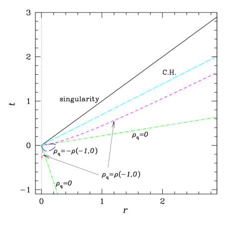
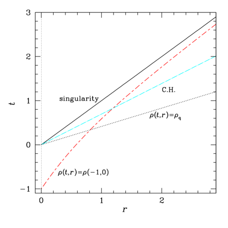
FIG. 1.: Plots of the lines $\rho_{\mbox{q}}=$ const in (a) and $\rho(t,r)=$ const and $\rho_{\mbox{q}}=\rho(t,r)$ in (b). Each line has the following meaning. Solid line: singularity, long-dashed-dotted line: Cauchy horizon, dashed line: $\rho_{\mbox{q}}=\rho(-1,0)$, dashed-dotted line: $\rho_{\mbox{q}}=0$, long-dashed line: $\rho_{\mbox{q}}=-\rho(-1,0)$, long-dashed-short-dashed line: $\rho(t,r)=\rho(-1,0)$, dotted line: $\rho_{\mbox{q}}=\rho(t,r)$.

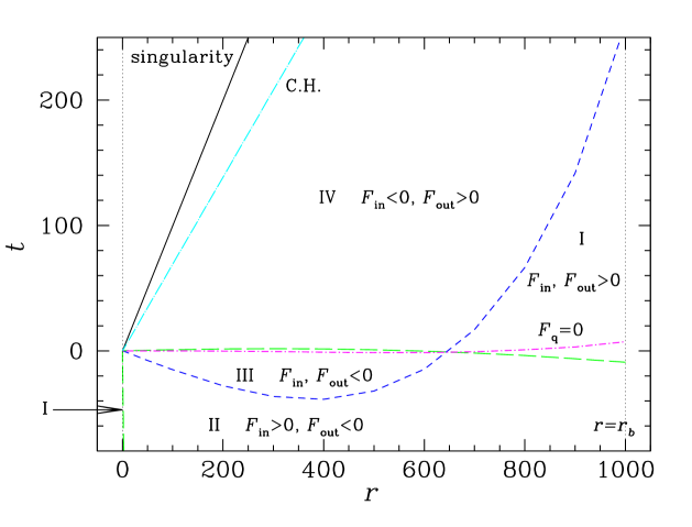
FIG. 2.: The solid line and long-dashed-dotted line correspond to the singularity and the Cauchy horizon, respectively. The dashed line denotes the line where the ingoing part of flux vanishes. On the long dashed lines the outgoing part vanishes. Region I, II, III, and IV correspond to positive in and out flux, positive in and negative out flux, negative in and out flux, and negative in and positive out flux, respectively. On the short-dashed-dotted line the observed net flux vanishes.

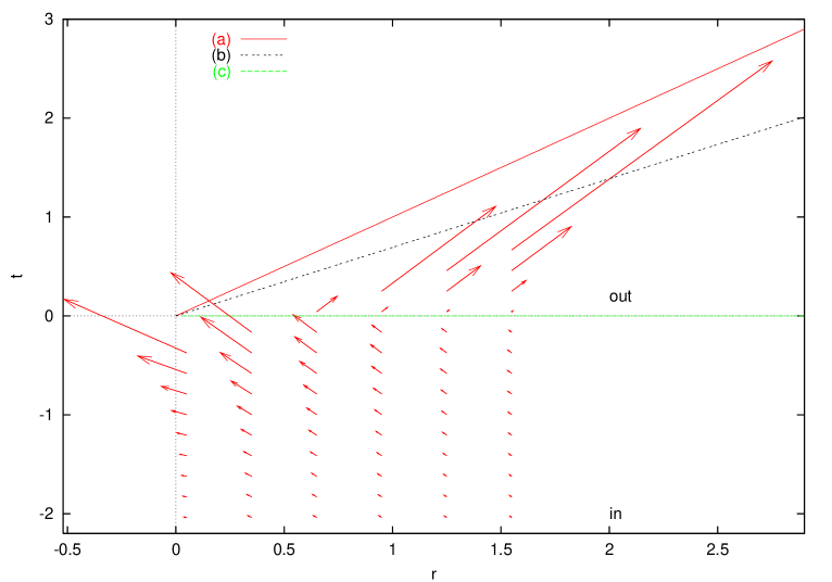
FIG. 3.: Schematic figure for the flux observed by comoving observer. Lines (a) and (b) correspond to the singularity and the Cauchy horizon, respectively. Line (c) denotes the line where the observed flux vanishes.

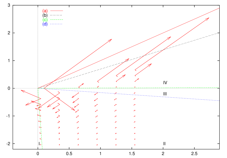
FIG. 4.: Schematic figure for the in and outgoing parts of flux observed by comoving observer. Lines (a) and (b) correspond to the singularity and the Cauchy horizon, respectively, Lines (c) and (d) denote the lines where outgoing part and ingoing part vanish respectively. Region I, II, III, and IV are similar to the ones in figure 2.

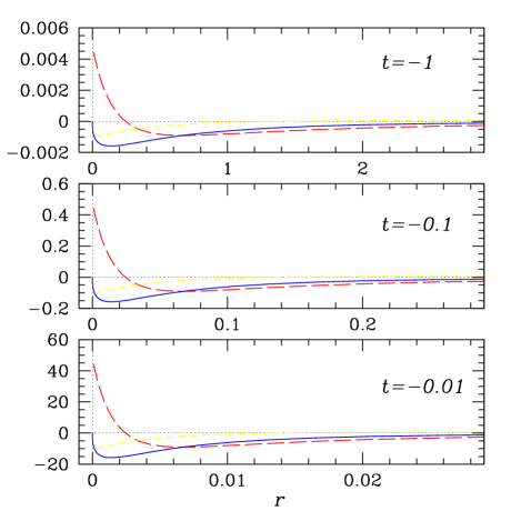
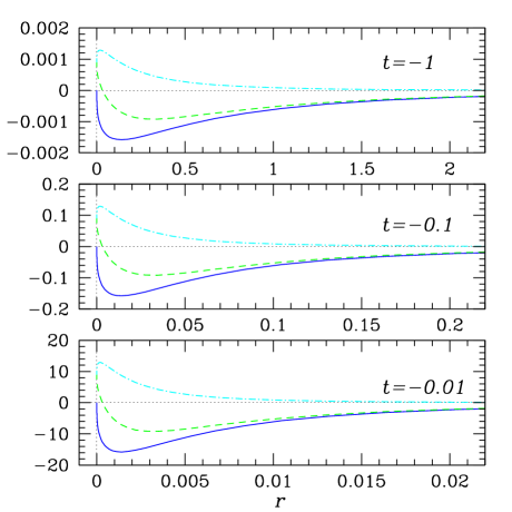
FIG. 5.: Plots of the quantum variables at $t=-1,-0.1,-0.01$. In (a) long-dashed lines denote $\rho_{\mbox{q}}$, solid lines denote $F_{\mbox{q}}$, and dashed lines denote quantum pressure $\langle T_{\mu\nu}\rangle n^{\mu}n^{\nu}$. In (b) solid lines denote flux $F_{\mbox{q}}$, dashed lines denote outgoing parts of flux $F_{\mbox{out}}$, and dashed-dotted lines denote ingoing parts of flux $F_{\mbox{in}}$.

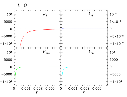
(a) $t=0$

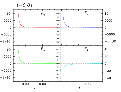
(b) $t=0.01$

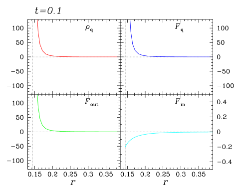
(c) $t=0.1$

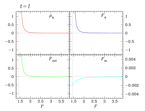
(d) $t=1$

FIG. 6.: Plots of the quantum variables at $t=0,0.01,0.1,1$ in (a), (b), (c), and (d) respectively. In each subfigure upper-left panel shows $\rho_{\mbox{q}}$, upper-right panel shows $F_{\mbox{q}}$, lower-left panel shows $F_{\mbox{out}}$, and lower right panel shows $F_{\mbox{in}}$. Vertical dotted lines in (b), (c) and (d) represent the Cauchy horizon.

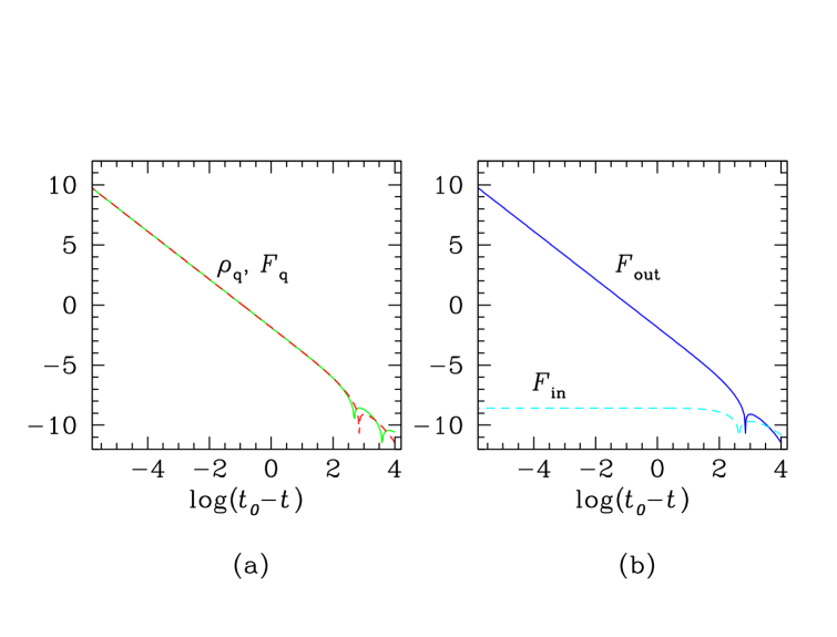
FIG. 7.: Logarithmic plots of the absolute values of quantum variables at the surface $r=r_{b}$.

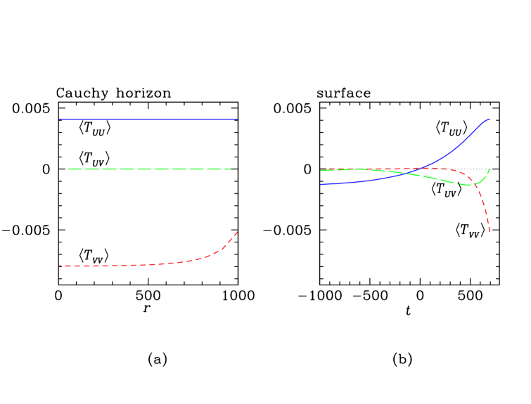
FIG. 8.: Plots of $\langle T_{UU}\rangle$, $\langle T_{VV}\rangle$, and $\langle T_{UV}\rangle$, at (a) Cauchy horizon, and at (b) $r=r_{b}$.

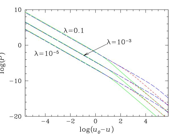
FIG. 9.: Radiated power received at the infinity. Upper lines correspond to $\lambda=0.1,$ , and middle lines correspond to $10^{-3}$, and lower lines correspond to $10^{-5}$. Solid, dashed, and long-dashed lines correspond to $r_{b}=10,10^{3},10^{5}$, respectively.

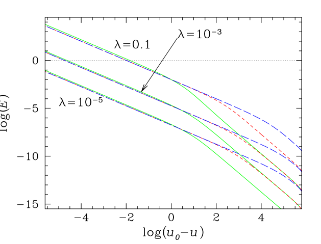
FIG. 10.: Integrated radiated power. Upper lines correspond to $\lambda=0.1,$ , and middle lines correspond to $10^{-3}$, and lower lines correspond to $10^{-5}$. Solid, dashed, and long-dashed lines correspond to $r_{b}=10,10^{3},10^{5}$, respectively.

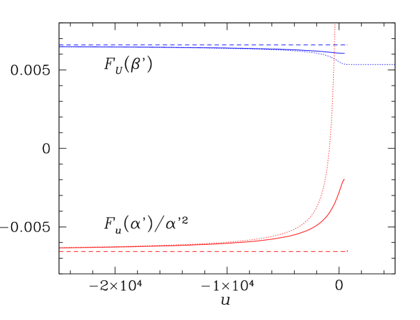
FIG. 11.: Plots of $F_{U}(\beta^{\prime})$ for upper lines, and $F_{u}(\alpha^{\prime})/\alpha^{\prime 2}$ for lower lines. Solid lines correspond to $\lambda=0.1$ and $r_{b}=10^{3}$ which is plotted to Cauchy horizon $u\approx 479.0390$, and dashed lines correspond to $\lambda=10^{-3}$ and $r_{b}=10^{5}$, which is plotted to the Cauchy horizon $u\approx 715.3728$. Dotted lines denote a black hole case $\lambda=1$ and $r_{b}=10^{2}$. In this case the retarded time at event horizon is $u=\infty$.

REFERENCES

- [1] Lemaître G, Ann. Soc. Sci. Bruxelles A53 (1993), 51
- [2] Tolman R C, Proc. Natl. Acad. Sci. U.S.A. 20 (1934), 169
- [3] Bondi H, Mon. Not. R. Astron. Soc. 107 (1947), 410
- [4] Eardley D Mand Smarr L, Phys. Rev. D19 (1979), 2239
- [5] Christodoulou D, Commun. Math. Phys. 93 (1984), 171
- [6] Newman R P C A, Class. Quantum Grav. 3 (1986), 527
- [7] Joshi P S and Dwivedi I H, Phys. Rev. D47 (1993), 5357
- [8] Jhingan S and Joshi P S, Annals of Israel Physical Society Vol. 13 (1997), 357
- [9] Wald R M, Gravitational collapse and cosmic censorship Preprint gr-qc/9710068
- [10] Penrose R, Black Holes and Relativistic Stars ed Wald R M (Chicago: The University of Chicago Press) p 103 (1998)
- [11] Ford L H and Parker L, Phys. Rev. D17 (1978) 1485
- [12] Hiscock W A , Williams L G and Eardley D M, Phys. Rev. D26 (1982) 751
- [13] Barve S, Singh T P, Vaz C and Witten L, Nucl. Phys. B532 (1998) 361
- [14] Harada T, Iguchi H and Nakao K, Phys. Rev. D61 (2000) 101502
- [15] Harada T, Iguchi H and Nakao K, Phys. Rev. D62 (2000) 084037
- [16] Singh T P and Vaz C, Phys. Lett. B481 (2000) 74
- [17] Iguchi H, Nakao K and Harada T, Phys. Rev. D57 (1998) 7262
- [18] Iguchi H, Harada T and Nakao K, Prog. Theor. Phys. 101 (1999) 1235
- [19] Iguchi H, Harada T and Nakao K, Prog. Theor. Phys. 103 (2000) 53
- [20] Nakao K, Iguchi H and Harada T, Phys. Rev. D63, 084003 (2001)
- [21] Joshi P S, Dadhich N K and Maartens R, Mod. Phys. Lett. A15 (2000) 991
- [22] Vaz C and Witten L, Phys. Lett. B 442 (1998) 90
- [23] Virbhadra K S, Narasimha D and Chitre S M, Astron. Astrophys. 337 (1998) 1
- [24] Harada T, Iguchi H, Nakao K, Singh T P, Tanaka T and Vaz C, gr-qc/0010101
- [25] Davies P C, Fulling S A and Unruh W G, Phys. Rev. D13, 2720 (1976)
- [26] Barve S, Singh T P, Vaz C and Witten L, Phys. Rev. D58, 104018 (1998)
- [27] Joshi P S and Singh T P, Phys. Rev. D51, 6778 (1995)