4-Dimensional optics, an alternative to relativity

Abstract

The starting point of this work is the principle that all movement of particles and photons in the observable Universe must follow geodesics of a 4-dimensional space where time intervals are always a measure of geodesic arc lengths, i.e. $c^{2}(\mathrm{d}t)^{2}=g_{\alpha\beta}\mathrm{d}x^{\alpha}\mathrm{d}x^{\beta}$, with $c$ is the speed of light in vacuum, $t$ time, $g_{\alpha\beta}$ and the metric tensor; $x^{\alpha}$ represents any of 4 space coordinates. The last 3 coordinates $(\alpha=1,2,3)$ are immediately associated with the usual physical space coordinates, while the first coordinate $(\alpha=0)$ is later found to be related to proper time. The work shows that this principle is applicable in several important situations and suggests that the underlying principle can, in fact, be used universally. Starting with special relativity it is shown that there is perfect mapping between the geodesics on Minkowski space-time and on this alternative space. The discussion than follows through light propagation in a refractive medium, and some cases of gravitation, including Schwartzschild’s outer metric. The last part of the presentation is dedicated to electromagnetic interaction and Maxwell’s equations, showing that there is a particular solution where one of the space dimensions is eliminated and the geodesics become equivalent to light rays in geometrical optics. A very brief discussion is made of the implications for wave-particle duality and quantization.

1 Introduction

General relativity is rooted on the consideration of Minkowski space-time, which is adequate for the formulation of special relativity. This space functions as tangent space in all other situations. A consequence of this approach is that all spaces of general relativity exhibit the characteristic $2$ signature of Minkowski space-time and can never be reduced to Euclidean space, which would be tangent to spaces of signature $4$. Our aim in this paper is to suggest that special relativity situations have an equally valid formulation in an Euclidean space, provided appropriate coordinates are chosen. Consequently, general situations can be studied in curved spaces having $4$ signature and ultimately can be reduced to an Euclidean tangent space. We have previously presented these concepts in unpublished form [1] but the present work extends and corrects important aspects.

With the new formulation we hope to deal with equations that are easier to solve, and generally with a simpler geometry. We will show that there is a prospect for unification between gravity and other interactions in nature, mainly by showing how electromagnetic interaction can be accommodated by the theory but also discussing some aspects related to quantum mechanics. There is one drawback, however. The reader must not expect one-to-one correspondence between events in relativistic space-time and points on the space we propose, because we will not be performing a change of coordinates, which could never change the space signature. The physical meaning of the points of this space will not be discussed here. The author thinks, however, that this is a subject that must be addressed in forthcoming work, in order to gain widespread acceptance of his proposal.

The legitimacy of the proposal stems from the following argument: All movement of particles must follow metric geodesics of the space when all the possible interactions are taken into account in building up the metric. Under these circumstances two different spaces are equally adequate for describing a particular kind of particle movement if it is possible to map geodesics from one space onto the other and furthermore it is possible to map points on corresponding geodesics of both spaces (note that this implies a one-to-one correspondence of geodesics between both spaces, but not a one-to-one correspondence of points). We will establish the validity of this principle in two particular situations of special relevance to general relativity.

First we will show that geodesics of Minkowski space-time can be mapped onto our proposed space, thus opening the way to the use of general curved spaces of signature $4$ for the representation of relativistic phenomena. Later we will show that the most important solution of general relativity for vacuum, namely Schwartzschild’s solution, also is amenable to geodesic mapping onto our proposed space. Besides establishing the legitimacy of the proposal through the discussion of the two mentioned cases, the paper introduces some concepts of quantum mechanics right from the flat space discussion, opening the road for future developments in this area.

It is shown that optical propagation, governed by Fermat’s principle, can be expressed as propagation in a 3-dimensional sub-space of the general 4-dimensional curved space, allowing optical interpretations of several relativistic phenomena, namely the interpretation of the gravitational field as a 4-dimensional refractive index. This contributes to the validation of the suggestion that quantum mechanical phenomena can be included in the theory as the homologous of optical modes in waveguides.

The final sections deal with the inclusion of electromagnetic interaction in the metric, thus allowing the expression of charged particle trajectories as movement along geodesics. The special case of photons is also analyzed and shown to fall perfectly within the previously discussed situation of optical propagation.

The whole theory is based on the hypothesis that there is always a space where particle and photon trajectories follow metric geodesics; this space is characterized by the universal interval

$$c^{2}(\mathrm{d}t)^{2}=g_{\alpha\beta}\mathrm{d}x^{\alpha}\mathrm{d}x^{\beta},$$ (1)

where $c$ is the speed of light in vacuum, $t$ is time, $x^{0}=\tau$ is a coordinate whose significance will have to be found and the $x^{i}$ $(i=1,2,3)$ correspond to the spatial cartesian coordinates $x,y,z$. This principle is applicable to all the observable Universe, i. e. the portion of the Universe within the light horizon; we make no predictions for any portions of the Universe which lay beyond the horizon. Eq. (1) establishes that the interval between two neighboring points of the space divided by the time interval between the same points equals the speed of light; this justifies the designation of optical space for this space.

It is possible to clarify the concept of optical space through embedding Minkowski space-time in a 5-dimensional space where the interval is defined by $\mathrm{d}s^{2}=\delta_{\alpha\beta}\mathrm{d}x^{\alpha}\mathrm{d}x^{\beta}-\mathrm{d}t^{2}$; on this 5-dimensional space the worldlines of particles follow geodesics of null interval. The same procedure can be extended to all situations in general relativity where the metric is diagonal. We go a step further when we propose that optical space can be applied even when the metric is non-diagonal, in which case null geodesics in 5-dimensional space no longer provide a connection between relativity and 4-dimensional optics.

2 Special relativity

The first case we consider deals with the translation of special relativity into our new proposed 4-dimensional optical space. This is characterized by the metric tensor

$$g_{\alpha\beta}=\delta_{\alpha\beta}.$$ (2)

We want to show that, by mapping the geodesics of Minkowski space-time to the geodesics of the optical space, there exists a relationship between displacements on corresponding geodesics and, therefore, any inertial movement that can be expressed in Minkowski space-time can also be expressed in optical space. We will use the index $\mathrm{O}$ to refer to the proposed space, $\mathrm{O}$ standing for optical.

Generally for any space, if the interval is expressed by $(\mathrm{d}s)^{2}=g_{\alpha\beta}\mathrm{d}x^{\alpha}\mathrm{d}x^{\beta}$, it is possible to derive the geodesic equation from the consideration of the Lagrangean $2L=g_{\alpha\beta}\dot{x}^{\alpha}\dot{x}^{\beta}$, with the ”dot” indicating derivation with respect to the arc length [2]. This Lagrangean is always constant equal to $1/2$.

In the optical space Eq. (1) establishes $\mathrm{d}t$ as the arc length and so a geodesic can be derived from the Lagrangean

$$2L_{\mathrm{O}}=\delta_{\alpha\beta}\dot{x}^{\alpha}\dot{x}^{\beta}=(\dot{\tau})^{2}+(\dot{x})^{2}+(\dot{y})^{2}+(\dot{z})^{2},$$ (3)

where the ”dot” is used to represent time derivatives, because time is associated with the interval.

The Lagrangean must be constant, equal to $1/2$, so we can write

$$(\dot{\tau})^{2}=1-(\dot{x})^{2}-(\dot{y})^{2}-(\dot{z})^{2}.$$ (4)

This is to be compared with the equation for a geodesic in Minkowski space-time, which can be derived from the interval

$$(\mathrm{d}s)^{2}=(\mathrm{d}t)^{2}-(\mathrm{d}{x})^{2}-(\mathrm{d}{y})^{2}-(\mathrm{d}{z})^{2}.$$ (5)

For time-like geodesics $\mathrm{d}s>0$ and so, for these geodesics, we can write

$$2L_{\mathrm{M}}=\left(\frac{\mathrm{d}t}{\mathrm{d}s}\right)^{2}-\left(\frac{\mathrm{d}x}{\mathrm{d}s}\right)^{2}-\left(\frac{\mathrm{d}y}{\mathrm{d}s}\right)^{2}-\left(\frac{\mathrm{d}z}{\mathrm{d}s}\right)^{2},$$ (6)

where the index $\mathrm{M}$ stands for Minkowski.

Eqs. (3) and (6) can represent the same lines if an identification is made between homologous quantities and $\mathrm{d}s=\mathrm{d}\tau$. In this instance both spaces verify the relation

$$\dot{\tau}=\sqrt{1-(\dot{x})^{2}-(\dot{y})^{2}-(\dot{z})^{2}}=\frac{1}{\gamma}~{}.$$ (7)

This equation establishes a relationship between $\tau$ and $t$, which is the same that exists between proper time and time for a moving particle in special relativity; we will therefore call proper time to the $\tau$ coordinate in optical space.

The equivalence between time-like geodesics in Minkowski space-time and the geodesics of optical space does not go very far in ensuring that particle movement can be studied in either space, whenever particles are under the influence of fields that deviate them from the 4-dimensional straight line geodesics. In fact the results are not equivalent, but this is no limitation because all deviation from geodesics is seen as an approximation, which should be preferably addressed through the search for the appropriate metric where particles will follow curved geodesics.

3 Mass scaling of coordinates

In the previous section we were concerned with geodesic equations with no concern for the mass of the actual particle moving along a geodesic. This is the usual relativistic standpoint where mass is considered to have a role as gravitational mass, inducing space curvature, which is separate from its role as inertial mass. Obviously the first role does not come into play in special relativity. We will adopt a somewhat different approach, consistent with our initial hypothesis that time intervals always measure arc length along the particle’s trajectory.

Based on the geodesic Lagrangean equation (3), we can define a conjugate momentum vector by

$$p_{\alpha}=\frac{\partial L_{O}}{\partial\dot{x}^{\alpha}}=\delta_{\alpha\beta}\dot{x}^{\beta}.$$ (8)

The momentum as defined is not any particle’s momentum but rather a geometrical quantity related to the space geodesics. If we wish the conjugate momentum to be related to the particle’s momentum, it is imperative to include mass in the metric or in the interval; we choose the first option. This can be achieved by a local coordinate scaling, which is required to exhibit an extremum at the precise location of the particle. The new metric is defined as

$$g_{\alpha\beta}=m^{2}\delta_{\alpha\beta},$$ (9)

with $m$ the particle’s rest mass. The movement Lagrangean is conveniently defined as $L=g_{\alpha\beta}\dot{x}^{\alpha}\dot{x}^{\beta}/2$, allowing us to define the particle’s 4-momentum as

$$p_{\alpha}=\frac{\partial L}{\partial\dot{x}^{\alpha}}=m^{2}\delta_{\alpha\beta}\dot{x}^{\beta}.$$ (10)

The extremum condition imposed on the scale factor $m$ ensures that it can be brought out of the derivative in Eq. (10). It will be noticed that the spatial components of the 4-momentum correspond precisely to the classical momentum when allowance is made for the mass scaling of the coordinates; $p_{0}$ can be shown to represent the particle’s kinetic energy.

There is a crucial difference between the covariant 4-momentum defined here and the contravariant homologous from special relativity. Our option of associating all trajectories with geodesics leads to the association between movement and geodesic Lagrangeans and consequently to the conjugate momentum being defined as a covariant vector.

Mass is here defined as a coordinate scale factor which allows us to maintain our initial hypothesis formulated in Eq. (1). With this modification the particle’s 4-velocity has now a magnitude equal to the speed of light divided by the mass; the special case of zero mass will be dealt with in section 5. It must be stressed that mass scaling is not necessarily a purely local effect. Wherever in space there are point masses, the local coordinates are scaled relative to the vacuum coordinates. Nothing is said about the effect mass has on the immediate vicinity of the traveling particle, although we already know from general relativity that this effect does exist. The consideration of coordinate scaling by the traveling particle’s mass will later be shown to bring more symmetry to the equations of general relativity and unification of the three roles of mass: Inertial mass, gravitational active mass and gravitational passive mass.

4 Waves in 4-dimensional optical space

One of the main advantages of the optical space formulation of relativity arises from the fact that it is a natural extension of the 3-dimensional space where ray and wave optics are two alternative ways of describing the same phenomena, wherever the geometrical optics approach is applicable.

We feel it is useful to accompany the relativistic discussion of particle trajectories with a discussion of wave propagation in the same space and draw some consequences which are pertinent to quantum mechanics. Considering Eq. (10) the geodesic equation for a particle of mass $m$ away from any fields can be written in terms of momentum as $\delta^{\alpha\beta}p_{\alpha}p_{\beta}=m^{2}$; if both sides of this equation are multiplied by the function $\psi=\mathrm{exp}(\mathrm{j}\,p_{\alpha}x^{\alpha})$, with $\mathrm{j}=\sqrt{-1}$, we get the wave equation

$$\delta^{\alpha\beta}\partial_{\alpha\beta}\psi=-m^{2}\psi,$$ (11)

which represents a stationary 4-dimensional plane wave pattern of spatial frequency $m$ and corresponding wavelength, designated by World wavelength, given by

$$\lambda_{w}=\frac{1}{m}.$$ (12)

We now consider the case of elementary particles to make an identification of $\lambda_{w}$ in the previous equation with Compton’s wavelength $\lambda_{w}=2\pi\hbar/{mc}$, which corresponds to writing the equation in normal rather than non-dimensional units.

If we temporarily remove the normalization of the speed of light, we will quickly recognize that the Compton frequency, given by $mc^{2}/\hbar$ is expressed by the same number as the particle’s mass when it is expressed in non-dimensional units.

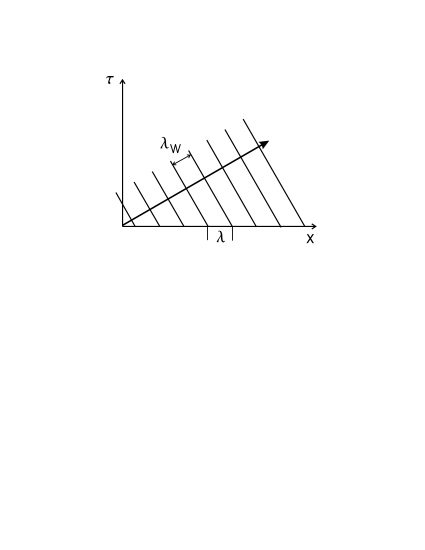
Figure 1: The moving particle has a world wavelength $\lambda_{w}=h/(mc)$ and a spatial wavelength $\lambda=h/(mv)$.

Fig. 1 illustrates a particle’s trajectory with superimposed wavefronts spaced $\lambda_{w}$ apart; these wavefronts intersect 3-dimensional physical space defining a wavelength $\lambda$ which, considering Eq. (7) is

$$\lambda=\frac{\lambda_{w}}{\sqrt{(\dot{x})^{2}(\dot{y})^{2}(\dot{z})^{2}}}=\frac{h}{p}~{};$$ (13)

$p$ represents the magnitude of the spatial component of momentum and this equation is exactly the definition of De Broglie’s wavelength. We have thus established a relation between Compton’s and De Broglie’s wavelength as a purely geometric one.

In the previous derivation we have assumed that particles move through 4-space with a 4-velocity with the magnitude of the speed of light and have an associated wavelength given by Eq. (12). If we now allow mass scaling of the coordinates as implied by Eq. (9), Eq. (11) is re-written as

$$\frac{1}{m^{2}}\delta^{\alpha\beta}\partial_{\alpha\beta}\psi=-\psi.$$ (14)

The spatial frequency becomes unity while the coordinates are scaled by the mass.

5 Lorentz equivalent transformations

Our approach to coordinate transformation between observers moving relative to each other is different from special relativity. While in the latter case the interval is given by Eq. (5), thus ensuring that a coordinate transformation preserves the interval and affects both spatial and time coordinates, our option of making time intervals measure geodesic arc length gives time a meaning independent of any coordinate transformation. We thus propose that Lorentz equivalent transformations between a ”fixed” or ”laboratory” frame and a moving frame are performed in two separate phases. The first phase is a tensorial coordinate transformation, which changes the coordinates keeping the origin fixed, with no influence in the way time is measured, while the second phase corresponds to a ”jump” into the moving frame, changing the metric but not the coordinates.

Making use the metric from Eq. (9) it is possible to express $\dot{x}^{0}$ in terms of $\dot{x}^{i}$, in a similar way to what was used to write Eq. (4):

$$m^{2}\left(\dot{x}^{0}\right)^{2}=1-m^{2}\delta_{ij}\dot{x}^{i}\dot{x}^{j}.$$ (15)

What is immediately obvious is that particles with zero mass, such as photons, cannot follow a geodesic of this space unless, as a limiting case, we force them to follow geodesics with $\mathrm{d}x^{0}=0$. We will deal with optical propagation in the next section; for now it will be sufficient to know that photons travel on the 3-dimensional $x^{i}$ space. Photons carry the value of the $x^{0}$ coordinate and can be used to synchronize all points in space to the observer’s own measurements of this coordinate. Following this argument we can say that a coordinate transformation must preserve the value of $\mathrm{d}x^{0}$. It will readily be seen that this statement is a direct equivalent to interval invariance in special relativity. On the other hand the time interval must also evaluate to the same value on all coordinate systems of the same frame, due to its definition as interval of the optical space.

Let us consider two unit mass observers $O$ and $\bar{O}$, the latter moving along one geodesic of $O$’s coordinate system. Let the geodesic equation have a parametric equation $x^{\alpha^{\prime}}(t)$. Our aim is to establish the coordinate transformation tensor between the two observers’ coordinate systems, ${\Lambda^{\bar{\mu}}}_{\alpha}=\partial x^{\bar{\mu}}/\partial x^{\alpha}$; we have already established that $\mathrm{d}x^{\bar{0}}=\mathrm{d}x^{0}$ and so it must be ${\Lambda^{\bar{0}}}_{0}=1$ and ${\Lambda^{\bar{0}}}_{i}=0$.

A photon traveling parallel to the $x^{1}$ direction follows a geodesic characterized by $\mathrm{d}t=\mathrm{d}x^{1}$ on $O$’s coordinates. On $\bar{O}$’s coordinates the photon will move parallel to $x^{\bar{1}}$ and so we can say that it is also $\mathrm{d}t=\mathrm{d}x^{\bar{1}}$. The same behaviour could be established for all three $(x^{i},~{}x^{\bar{i}})$ coordinate pairs and we conclude that ${\Lambda^{\bar{i}}}_{i}=1$.

Consider now two points $\mathcal{P}_{1}$ and $\mathcal{P}_{2}$ on a line parallel to $x^{0}$ axis in $O$’s coordinates, separated by a time interval $\mathrm{d}t=\mathrm{d}x^{0}$. On $\bar{O}$’s coordinates it will be

$$\mathrm{d}x^{\bar{i}}=-\dot{x}^{i^{\prime}}\mathrm{d}t=\frac{\dot{x}^{i^{\prime}}}{\dot{x}^{0^{\prime}}}~{}\mathrm{d}x^{0},$$ (16)

allowing us to conclude that ${\Lambda^{\bar{i}}}_{0}=-\dot{x}^{i^{\prime}}/\dot{x}^{0^{\prime}}=-\breve{x}^{i}$, where the notation $\breve{x}^{i}$ is used for derivation with respect to $\tau$. Fig. 2 shows graphically the relation between the two coordinate systems.

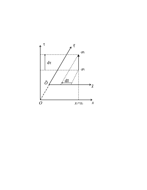
Figure 2: The worldline of moving observer $\bar{O}$ coincides with the $\bar{\tau}$ axis, while the $\bar{x}$ axis stays parallel to the $x$ axis. A displacement parallel to axis $\tau$ implies both $\bar{x}$ and $\bar{\tau}$ components in the moving frame.

The coordinate transformation tensor between $x^{\alpha}$ and $x^{\bar{\mu}}$ is consequently defined as

$${\Lambda^{\bar{\mu}}}_{\alpha}=\left[\begin{array}[]{cccc}1&0&0&0\\ -\breve{x}^{1^{\prime}}&1&0&0\\ -\breve{x}^{2^{\prime}}&0&1&0\\ -\breve{x}^{3^{\prime}}&0&0&1\end{array}\right].$$ (17)

The reverse transformation is obtained changing the sign of $-\breve{x}^{i^{\prime}}$.

We are now in position to evaluate the metric for $\bar{O}$’s coordinates

$$g_{\bar{\mu}\bar{\nu}}={\Lambda^{\alpha}}_{\bar{\mu}}{\Lambda^{\beta}}_{\bar{\nu}}g_{\alpha\beta};$$ (18)

after evaluation we get

$$g_{\bar{\mu}\bar{\nu}}=\left[\begin{array}[]{cccc}1+\delta_{a^{\prime}b^{\prime}}\breve{x}^{a^{\prime}}\breve{x}^{b^{\prime}}&\breve{x}^{1^{\prime}}&\breve{x}^{2^{\prime}}&-\breve{x}^{3^{\prime}}\\ \breve{x}^{1^{\prime}}&1&0&0\\ \breve{x}^{2^{\prime}}&0&1&0\\ \breve{x}^{3^{\prime}}&0&0&1\end{array}\right].$$ (19)

The metric given by the previous equation will evaluate time in $\bar{O}$’s coordinates in a frame which is fixed relative to $O$, that is, this is still time as measured by observer $O$. Observer $\bar{O}$ will measure time intervals $\mathrm{d}\bar{t}$ in his own frame and so, although the coordinates are the same as they were in $O$’s frame, time is evaluated with the Kronecker metric $\delta_{\bar{\mu}\bar{\nu}}$ instead of metric given by Eq. (19).

Mathematically the metric replacement corresponds to the identity

$$\delta_{\bar{\alpha}\bar{\beta}}=\left(g_{\bar{\mu}\bar{\nu}}\right)^{-1}g_{\bar{\mu}\bar{\nu}};$$ (20)

this operation will be used later to derive the metric for electromagnetic interaction. We note that this transformation preserves the essential relationship of special relativity, i. e. for a unit mass particle $\mathrm{d}\bar{t}^{2}-\delta_{\bar{i}\bar{j}}\mathrm{d}x^{\bar{i}}\mathrm{d}x^{\bar{j}}=\mathrm{d}t^{2}-\delta_{ij}\mathrm{d}x^{i}\mathrm{d}x^{j}$.

6 Optical propagation

Let us now consider the situation where the metric has the form

$$g_{0\alpha}=g_{\alpha 0}=0,~{}~{}g_{ij}=n^{2}\delta_{ij}~{}(i,j\neq 0),$$ (21)

with $n$ a function of the coordinates. This is really the metric of a 3-dimensional subspace where the coordinate $x^{0}$ does not intervene. Eq. (1) becomes

$$(\mathrm{d}t)^{2}=n^{2}\left[(\mathrm{d}x)^{2}+(\mathrm{d}y)^{2}+(\mathrm{d}z)^{2}\right],$$ (22)

which is readily seen to lead to Fermat’s principle when this variational principle is written

$$\delta\int n\mathrm{d}\sigma=0,$$ (23)

with $n$ the refractive index of the optical medium and $\mathrm{d}\sigma$ the interval in Euclidean space given by

$$\mathrm{d}\sigma=\sqrt{(\mathrm{d}x)^{2}+(\mathrm{d}y)^{2}+(\mathrm{d}z)^{2}}.$$ (24)

Obviously this space supports 3-dimensional waves, as it is none other than the usual optical space where all the rules of optical propagation are well established.

The propagation speed is $1/n$ and the corresponding wavelength is $\lambda=h/nE$, with $E$ the photon energy.

7 Gravitation

Stationary vacuum solutions for gravitational field are expected to have a null Ricci tensor, meaning that a suitable coordinate change will produce a diagonal metric with just $1$ and $-1$ elements in the diagonal [2]; this combined with the characteristic $4$ signature of the optical space we are using means that these solutions must be conformal transformations of an Euclidean metric. We define these solutions by the general metric

$$g_{\alpha\beta}=n^{2}\delta_{\alpha\beta},$$ (25)

where $n$ is a function of the coordinates. This is a 4D extension of the optical 3D sub-space discussed in the previous section and further justifies the choice of optical space as the designation for our proposed 4-space.

Similarly to what was done for the Minkowski space-time, it is possible to map the geodesics of this particular situation to time-like geodesics of general relativity’s curved space-time for vacuum. Eq. (1) now becomes

$$(\mathrm{d}t)^{2}=n^{2}\left(\mathrm{d}\tau^{2}+\mathrm{d}x^{2}+\mathrm{d}y^{2}+\mathrm{d}z^{2}\right);$$ (26)

which can be arranged as

$$(\mathrm{d}s)^{2}=\frac{1}{n}~{}(\mathrm{d}t)^{2}-n\left(\mathrm{d}x^{2}+\mathrm{d}y^{2}+\mathrm{d}z^{2}\right).$$ (27)

Recalling Eq. (27) and making $(\mathrm{d}s)^{2}=n(\mathrm{d}\tau)^{2}$, we can invoke the Lagrangean unity to arrive at the relation

$$\dot{\tau}=\sqrt{\frac{1}{n^{2}}-\dot{x}^{2}-\dot{y}^{2}-\dot{z}^{2}}=\sqrt{\frac{1}{n^{2}}-v^{2}}.$$ (28)

Eq. (25) is obtained from Eq. (2) by multiplication of the right-hand side by $n^{2}$, equivalent to a position dependent scale factor. When $n$ is a constant independent of the coordinates the space becomes flat and only the relationship between time and space intervals is altered; this is the same effect that was produced by the particle’s own mass in the special relativity discussion. We are then led to conclude that mass must be a source of space curvature leading eventually to Einstein’s equations modified for the optical space. This will be the subject of a future publication and will not be pursued in the present paper.

Naturally it is possible to extend Fermat’s principle to this 4-dimensional space, deriving particle’s trajectories as if they were 4-dimensional light rays. Just as the refractive index does in optics, gravity can be interpreted as reducing the 4-dimensional wavelength of the particles relative to its $1/m$ value away from other masses. Similarly to optics, the refractive index approach is an alternative to space curvature.

Scwartzschild derived the general vacuum solution of Einstein’s equation for a spherically symmetric situation [3, 2], which can be written

$$\mathrm{d}s^{2}=\frac{1}{n}\,\mathrm{d}t^{2}+n\mathrm{d}r^{2}+r^{2}\left(\mathrm{d}\theta^{2}+\sin^{2}\theta\mathrm{d}\phi^{2}\right),$$ (29)

where $r$, $\theta$, $\phi$ are the spherical coordinates and

$$\frac{1}{n}=\left(1-\frac{M}{r}\right),$$ (30)

with $M$ the mass of a large body and non-dimensional units in use. The equivalence to optical space can be made by setting $\mathrm{d}t$ as the interval

$$\mathrm{d}t^{2}=n^{2}\left(\mathrm{d}\tau^{2}+\mathrm{d}r^{2}\right)+nr^{2}\left(\mathrm{d}\theta^{2}+\sin^{2}\theta\mathrm{d}\phi^{2}\right).$$ (31)

The fact that this is not in the form of Eq. (26) can be attributed, we believe, to the fact that Schwartzschild’s metric is a direct consequence of the hyperbolic space and is certainly not a necessity in a non-hyperbolic one. There are some implications for the existence and characteristics of black holes which we don’t discuss here.

Newtonian mechanics tells us that the gravitational pull force of a large body, considered fixed with mass $M$, over a much smaller body of mass $m$ is

$$\vec{f}=m\nabla V,$$ (32)

where the arrows were used to denote vectors in 3D space and the ”nabla” operator has its usual 3-dimensional meaning; $V$ is the gravitational potential given by

$$V=\frac{GM}{r};$$ (33)

$r$ is distance between the two bodies. The constant $G$ was left in the expression so that it would appear in its most traditional form, but it should be removed with non-dimensional units.

If the moving body is under the single influence of the gravitational field, the rate of change of its momentum will equal this force and so we write $\mathrm{d}^{2}\vec{r}/\mathrm{d}t^{2}=\nabla V$; $\vec{r}$ is the position vector. If we use mass scaling of the coordinates, introduced before, the spatial components of the momentum must appear as $m^{2}\delta_{ij}\dot{x}^{j}$; the gradient is also affected by the scaling and we expect it to appear as $\partial_{i}V/m$. Using primed indices to denote unscaled coordinates it is

$$\delta_{i^{\prime}j^{\prime}}\ddot{x}^{j^{\prime}}=\partial_{i^{\prime}}V,$$ (34)

$$m^{2}\delta_{ij}\ddot{x}^{j}=\partial_{i}V.$$ (35)

We are looking for a Lagrangean of the type $2L=n^{2}\delta_{\alpha\beta}\dot{x}^{\alpha}\dot{x}^{\beta}$ where $n$ is a function of the radial coordinate only. In Cartesian coordinates it is

$$2L=n^{2}\delta_{\alpha\beta}\dot{x}^{\alpha}\dot{x}^{\beta}.$$ (36)

This lagrangean must be consistent with the non-relativistic form of the gravitational force and the resulting metric must be asymptotically flat.

If we derive the Euler-Lagrange’s equations for the 3 spatial dimensions we get

$$n\delta_{a\beta}\ddot{x}^{\beta}=\partial_{a}n\delta_{\alpha\beta}\dot{x}^{\alpha}\dot{x}^{\beta}=\partial_{a}n\left[\left(\dot{x}^{0}\right)^{2}+\delta_{ij}\dot{x}^{i}\dot{x}^{j}\right].$$ (37)

From Eq. (36) we take $\delta_{ij}\dot{x}^{i}\dot{x}^{j}=1/n^{2}-(\dot{x}^{0})^{2}$, to be replaced above:

$$n^{2}\delta_{a\beta}\ddot{x}^{\beta}=\frac{\partial_{a}n}{n}.$$ (38)

It is now convenient to make the replacement $n=m\eta$, so that the previous equation becomes

$$m^{2}\eta_{r}^{2}\delta_{a\beta}\ddot{x}^{\beta}=\frac{\partial_{a}\eta_{r}}{\eta_{r}}.$$ (39)

If Eq. (39) is to produce the same results as Eq. (35) at appreciable distances from the central body, $\eta$ must be a function of $r$ that when expanded in series of $1/r$ has the first two terms $1+M/r$ in non-dimensional units. An interesting possibility is the function

$$\eta=\mathrm{e}^{V}=\mathrm{e}^{M/r}.$$ (40)

The second members of the relativistic and Newtonian equations are now equal and the first members will be equivalent in non-relativistic situations. So compatibility with Newtonian mechanics is ensured. In Ref. [4] we used this type of gravitational field to discuss some important gravitational anomalies.

8 Electrostatic field

Let us now turn our attention to electrostatic field by consideration of the electrostatic force on a charged particle of mass $m$ and electric charge $q$. This force can be written as

$$\vec{f}=-q\nabla V.$$ (41)

Here $V$ is the electrostatic potential such that $\nabla V=\vec{E}$ with $\vec{E}$ the electric field. We use a procedure similar to what was used in the previous section to say that if the particle is under the single influence of the electrostatic force we must have $m~{}\mathrm{d}^{2}\vec{r}/\mathrm{d}t^{2}=-q\nabla V$. Again after coordinate scaling it is

$$m^{2}\delta_{ab}\ddot{x}^{b}=-\frac{q}{m}~{}\partial_{a}V.$$ (42)

We are now looking for a Lagrangean which includes mass in the spatial components of the momentum and the field in the 0th component.

$$2L=g_{00}\left(\dot{x}^{0}\right)^{2}+m^{2}\delta_{ab}\dot{x}^{a}\dot{x}^{b};$$ (43)

this must be consistent with the non-relativistic form of the electrostatic force. For speeds much smaller than the speed of light $(\dot{x}^{0})^{2}\simeq 1/g_{00}$. If we derive the Euler-Lagrange’s equations for the 3 spatial dimensions we get

$$2m^{2}\delta_{ij}\ddot{x}^{j}=\partial_{i}g_{00}\left(\dot{x}^{0}\right)^{2};$$ (44)

one possible solution to get compatibility between Eqs. (42 and 44) is to make $g_{00}=m^{2}\mathrm{exp}(-2qV/m)$.

The metric for the electrostatic situation follows directly

$$g_{\alpha\beta}=m^{2}\left[\begin{array}[]{cccc}V_{0}&0&0&0\\ 0&1&0&0\\ 0&0&1&0\\ 0&0&0&1\end{array}\right],$$ (45)

with $V_{0}=\mathrm{exp}(-2qV/m)$.

The geodesics of the space defined above correctly predict particle movement under an electrostatic field in the non-relativistic situation and provide a plausible generalization for the relativistic cases. The relativistic prediction is not entirely coincident with those based on general relativity, which allow deviation from geodesics. The proposed optical space’s predictions are equivalent to general relativity only in those cases when movements follow geodesics; the allowance that is made in general relativity for parallel transport can also be made here as an approximation to the desired approach, which involves finding the metric for each and every particle movement. When particles are allowed to deviate from geodesics we do not expect a perfect match between results obtained in the optical and relativistic spaces.

The parallel with optics can now be completed recalling that we associate to every elementary particle its Compton frequency $f=mc^{2}/h$, as suggested before. The particle’s worldline is then marked by the Compton wavelength and 3D projection of this wavelength is found to define the De Broglie wavelength, as we saw earlier. When the electric or gravitational potential exhibit a minimum restricted to a small region of space, the particle can enter a closed orbit, which is the 3-dimensional counterpart of an helix shaped worldline. This type of worldline is analogous to a light ray confined to an optical waveguide. It is no wonder that propagation modes start to develop as the orbit diameter decreases, which are the 4D counterparts of quantum phenomena.

The wave equation for an elementary particle under both electric and gravitational field can be written

$$\frac{1}{V_{0}}\,\partial_{00}\psi+\delta^{ij}\partial_{ij}\psi=-m^{2}n^{2}\psi.$$ (46)

If the partial derivative $\partial_{0}\psi$ is expressed in terms of $\partial_{t}{\psi}$ and $\partial_{i}\psi$ through the metric, the equation will become a 3-dimensional wave equation which has been shown to degenerate in Schrödinger equation in the non-relativistic limit [5]. Outside this limit Eq. (46) will produce a relativistic 3D wave equation which is expected to be compatible with quantization due to electrostatic force.

9 Electromagnetism and light propagation

In a non-relativistic situation the Lorentz force on a moving particle of electric charge $q$ can be written $\vec{f}=q(\vec{E}+\vec{v}\times\vec{B})$, where the arrows were used to identify vectors in 3D non-relativistic mechanics, $\vec{E}$ is the electric field, $\vec{B}$ the magnetic field and $\vec{v}$ the particle’s speed. We now use Einstein’s argument [7] to say that if we place our frame on the moving particle this will be under the influence of an electrostatic force, due to the zeroing of the velocity on the Lorentz force expression. The electromagnetic force should then be the consequence of expressing the electrostatic force on a frame that is not moving with the particle.

We then use Eqs. (18 and 20) to transform the metric of Eq. (45) into the electromagnetic situation; the bar over the indices indicates the particle’s frame.

$$g_{\alpha\beta}=\left(g^{\bar{\mu}\bar{\nu}}\right)^{-1}g_{\bar{\mu}\bar{\nu}}=m^{2}\left[\begin{array}[]{cccc}V_{0}&V_{1}&V_{2}&V_{3}\\ V_{1}&1+\frac{(V_{1})^{2}}{V_{0}}&\frac{V_{1}V_{2}}{V_{0}}&\frac{V_{1}V_{3}}{V_{0}}\\ V_{2}&\frac{V_{1}V_{2}}{V_{0}}&1+\frac{(V_{2})^{2}}{V_{0}}&\frac{V_{2}V_{3}}{V_{0}}\\ V_{3}&\frac{V_{1}V_{3}}{V_{0}}&\frac{V_{2}V_{3}}{V_{0}}&1+\frac{(V_{3})^{2}}{V_{0}}\end{array}\right],$$ (47)

with

$$V_{0}=e^{-2qV/m}~{},~{}~{}~{}~{}V_{i}=V_{0}\frac{\dot{x}^{i^{\prime}}}{\dot{x}^{0^{\prime}}}.$$ (48)

Note that the $\dot{x}^{\alpha^{\prime}}$ of the previous equation refer to the movement of the frame where the Lorentz force becomes purely electrostatic and not to any particle’s movement.

We can now write the Lagrangean for a geodesic of the electromagnetic space using Eq. (47), the $x^{\alpha}$ representing the inertial movement of a particle under electromagnetic force:

$$L=g_{\alpha\beta}\dot{x}^{\alpha}\dot{x}^{\beta}.$$ (49)

The electromagnetic field can be associated to an anti-symmetric tensor $F_{\alpha\beta}$ such that [2]

$$F_{\alpha\beta}=\left[\begin{array}[]{cccc}0&-E_{1}&-E_{2}&-E_{3}\\ E_{1}&0&B_{3}&-B_{2}\\ E_{2}&-B_{3}&0&B_{1}\\ E_{3}&B_{2}&-B_{1}&0\end{array}\right].$$ (50)

$F_{\alpha\beta}$ can be obtained from $V_{\alpha}$ through

$$F_{\alpha\beta}=\frac{m}{2qV_{0}}\left(\partial_{\alpha}V_{\beta}-\partial_{\beta}V_{\alpha}\right).$$ (51)

If we start with the field tensor referred to a frame where the Lorentz force becomes purely electrostatic and use the transformation tensor to refer to the fixed frame we can write

$$F_{\alpha\beta}={\Lambda_{\alpha}}^{\bar{\mu}}{\Lambda_{\beta}}^{\bar{\nu}}F_{\bar{\mu}\bar{\nu}},$$ (52)

with

$$F_{\bar{\mu}\bar{\nu}}=\left[\begin{array}[]{cccc}0&-E_{1}&-E_{2}&-E_{3}\\ E_{1}&0&0&0\\ E_{2}&0&0&0\\ E_{3}&0&0&0\end{array}\right];$$ (53)

the final result is

$$F_{\alpha\beta}=\left[\begin{array}[]{cccc}0&-E_{1}&-E_{2}&-E_{3}\\ E_{1}&0&E_{2}\breve{x}^{1}-E_{1}\breve{x}^{2}&E_{3}\breve{x}^{1}-E_{1}\breve{x}^{3}\\ E_{2}&E_{1}\breve{x}^{2}-E_{2}\breve{x}^{1}&0&E_{3}\breve{x}^{2}-E_{2}\breve{x}^{3}\\ E_{3}&E_{1}\breve{x}^{3}-E_{3}\breve{x}^{1}&E_{2}\breve{x}^{3}-E_{3}\breve{x}^{2}&0\end{array}\right].$$ (54)

Let us look at a particular solution pertaining to the propagation of electromagnetic radiation, which should have a null component of momentum along the $x^{0}$ direction. Considering Eq. (49) the first component of the momentum vector is

$$p_{0}=2m^{2}V_{\alpha}\dot{x}^{\alpha}=2m^{2}\left(V_{0}\dot{x}^{0}+V_{i}\dot{x}^{i}\right).$$ (55)

The particular solution we are searching calls for $p_{0}=0$

$$\dot{x}^{0}=-\frac{V_{i}\dot{x}^{i}}{V_{0}}.$$ (56)

We note immediately that if $x^{0}$ is not to grow indefinitely it must average zero and so we postulate that it is a periodic function of $t$. Eq. (56) can be replaced in Eq. (49)

$$L=m^{2}\delta_{ij}\dot{x}^{i}\dot{x}^{j}.$$ (57)

The result is a Lagrangean which depends only on the spatial variables and is a special case of the optical propagation condition given by Eq. (21); here $m^{2}$ plays the role of the refractive index. In fact an optical medium is expected to have a complex metric and the final refractive index will be the result of all the contributions, including the mass distribution. It is noticeable that if we had derived Eq. (57) in a gravitational field situation, this would appear as an $n^{2}$ factor in the second member, accounting for the redshift induced by gravity and light bending near massive bodies.

10 Conclusions and further developments

We proposed two main premises for relativistic mechanics as 4-dimensional optics, these being: ”All trajectories will follow geodesics in a suitably defined 4-dimensional space” and ”Geodesic or trajectory length can be measured by the time interval multiplied by the speed of light in vacuum.” We find it virtually impossible to demonstrate the validity of those premises and so we chose to show that they will produce the same consequences as General relativity in two particularly important situations, namely Minkowski and Scwartzschild metrics. The equivalence to General relativity was based on the argument that ”If particle’s trajectories follow metric geodesics, the mapping of geodesics between two spaces is a sufficient condition for those spaces to be equivalent from the point of view of particle movement.” We derived an exponential gravitational field compatible with Newtonian mechanics in non-relativistic situations, which we believe is more appropriate than Schwartzschild’s in 4-dimensional optics.

We also showed that optical propagation follows the same rules as particle trajectories but is restricted to a 3-dimensional sub-space. The association of a 4-dimensional wave equation to the trajectories of elementary particles, in a similar way to the 3-dimensional waves associated with photons, allowed the derivation of an important connection between Compton’s and De Broglie’s wavelengths as a purely geometrical one. Quantization was also shown to result whenever particles are restricted to small orbits or to orbits under strong fields.

The Lorentz force and electromagnetism were also shown to be compatible with the initial premises, allowing the prediction of trajectories under electromagnetic interaction and the connection between light propagation in optical media, the metric and optical refractive index.

Two main directions of forthcoming work are expected to produce results and contribute to validate the theory. One area of work will try to establish equations equivalent to Einstein’s in this new formulation. This will be a direct consequence of the coordinate scaling by the mass that was introduced in this paper for point particles. A straightforward generalization will replace mass by mass density and coordinate scaling by curvature. It is expected that this line of work will yield further validation but most of all it is expected to lead to equations that are easier to solve then Einstein’s in a variety of situations.

A different aspect will be the exploitation of the 4-dimensional wave equation, namely for particle interactions. We feel that we have only skimmed the surface of this rich field and that there is scope for a large number of important results integrating gravitation with electromagnetism and eventually with all the known particle interactions.

References

- [1] José B. Almeida. An alternative to Minkowski space-time. In GR 16, Durban, South Africa, 2001. gr-qc/0104029.
- [2] Ray D’Inverno. Introducing Einstein’s Relativity. Clarendon Press, Oxford, 1996.
- [3] K. Schwartzschild. On the gravitational field of a mass point according to Einstein’s theory. Sitzungsberichte der Königlich Preussischen Akademie der Wissenschaften zu Berlin, Phys.-Math. Klasse, pages 189–196, 1916. physics/9905030.
- [4] José B. Almeida. On the anomalies of gravity. gr-qc/0105036, 2001.
- [5] José B. Almeida. Optical interpretation of special relativity and quantum mechanics. In OSA Annual Meeting, Providence, RI, 2000. physics/0010076.
- [6] H. A. Lorentz, A. Einstein, and Minkowski, editors. The Principle of Relativity, volume 1 of Textos Fundamentais da Física Moderna, Lisboa, 1983. Fundação Calouste Gulbenkian. O Princípio da Relatividade, Portuguese translation.
- [7] A. Einstein. About the electrodynamics of moving bodies. In Lorentz et al. [6], pages 47–86. Portuguese translation of Ann. Phys. 17 (1905).