Accelerated sources in de Sitter spacetime and the insufficiency of retarded fields

Abstract

The scalar and electromagnetic fields produced by the geodesic and uniformly accelerated discrete charges in de Sitter spacetime are constructed by employing the conformal relation between de Sitter and Minkowski space. Special attention is paid to new effects arising in spacetimes which, like de Sitter space, have spacelike conformal infinities. Under the presence of particle and event horizons, purely retarded fields (appropriately defined) become necessarily singular or even cannot be constructed at the “creation light cones” — future light cones of the “points” at which the sources “enter” the universe. We construct smooth (outside the sources) fields involving both retarded and advanced effects, and analyze the fields in detail in case of (i) scalar monopoles, (ii) electromagnetic monopoles, and (iii) electromagnetic rigid and geodesic dipoles.

PACS: 04.20.-q, 04.40.-b, 98.80.Hw, 03.50.-z

1 Introduction

The de Sitter’s 1917 solution of the vacuum Einstein equations with a positive cosmological constant $\Lambda$, in which freely moving test particles accelerate away from one another, played a crucial role in the acceptance of expanding standard cosmological models at the end of the 1920s [1, 2]. It reappeared as the basic arena in steady-state cosmology in the 1950s, and it has been resurrected in cosmology again in the context of inflationary theory since the 1980’s [2]. de Sitter spacetime represents the “asymptotic state” of cosmological models with $\Lambda>0$ [3].

Since de Sitter space shares with Minkowski space the property of being maximally symmetric but has a nonvanishing constant positive curvature and nontrivial global properties, it has been widely used in numerous works studying the effects of curvature in quantum field theory and particle physics (see, e.g., Ref. [4] for references). Recently, its counterpart with a constant negative curvature, anti–de Sitter space, has received much attention again from quantum field and string theorists (e.g. Ref. [5]).

These three maximally symmetric spacetimes of constant curvature also played a most important role in gaining many valuable insights in mathematical relativity. For example, both the particle (cosmological) horizons and the event horizons for geodesic observers occur in de Sitter spacetime, and the Cauchy horizons in anti–de Sitter space (e.g. Ref. [6]). The existence of the past event horizons of the worldlines of sources producing fields on de Sitter background is of crucial significance for the structure of the fields.

The existence of the particle and event horizons is intimately related to the fact that de Sitter spacetime has, in contrast with Minkowski spacetime, two spacelike infinities — past and future — at which all timelike and null worldlines start and end [6]. Since the pioneering work of Penrose [7, 8] it has been well known that Minkowski, de Sitter, and anti–de Sitter spacetimes, being conformally flat, can be represented as parts of the (conformally flat) Einstein static universe. However, the causal structure of these three spaces is globally very different. The causal character of the conformal boundary ${\mathcal{I}}$ to the physical spacetime that represents the endpoints at infinity reached by infinitely extended null geodesics, depends on the sign of $\Lambda$. In Minkowski space, these are null hypersurfaces — future and past null infinity, ${\mathcal{I}}^{+}$ and ${\mathcal{I}}^{-}$. In de Sitter space, both ${\mathcal{I}}^{+}$ and ${\mathcal{I}}^{-}$ are spacelike; in anti–de Sitter space the conformal infinity ${\mathcal{I}}$ is not the disjoint union of two hypersurfaces, and it is timelike.

Towards the end of his 1963 Les Houches lectures [9], Penrose discusses briefly the zero rest-mass free fields with spin $s$ in cosmological (not necessarily de Sitter) backgrounds. At a given point $P$, not too far from ${\mathcal{I}}^{-}$, say, the field can be expressed as an integral over quantities defined on the intersection of the past null cone of $P$ and ${\mathcal{I}}^{-}$ (“free incoming radiation field”) plus contributions from sources whose worldlines intersect the past null cone. However, the concept of “incoming radiation field” at ${\mathcal{I}}^{-}$ depends on the position of $P$ if ${\mathcal{I}}^{-}$ is spacelike [9, 10]. If there should be no incoming radiation at ${\mathcal{I}}^{-}$ with respect to all “origins $P$”, all components of the fields must vanish at ${\mathcal{I}}^{-}$. Imagine that spacelike ${\mathcal{I}}^{-}$ is met by the worldlines of discrete sources. Then there will be points $P$ near ${\mathcal{I}}^{-}$ whose past null cones will not cross the worldlines — see Fig. 1. The field at $P$ should vanish if an incoming field is absent. This, however, is not possible since the “Coulomb-type” part of the field of the sources cannot vanish there (as follows from Gauss’s law). Penrose [9] thus concludes that “if there is a particle horizon, then purely retarded fields of spin $s>\frac{1}{2}$ do not exist for general source distributions.” (The restriction on $s$ follows from the number of arbitrarily specifiable initial data for the field with spin $s$ — see Ref. [9].) Penrose also emphasized that the result depends on the definition of advanced and retarded fields, and “the application of the result to actual physical models is not at all clear cut … .” This observation was reported in a somewhat more detail at the meeting on “the nature of time” [11], with an appended discussion (in which, among others, Bondi, Feynman, and Wheeler participated) but technically it was not developed futher since 1963. In a much later monograph Penrose and Rindler [10] discuss (see p. 363 in Vol. II) the fact that the radiation field is “less invariantly” defined when ${\mathcal{I}}$ is spacelike than when it is null, but no comments or references are given there on the absence of “purely retarded fields.”

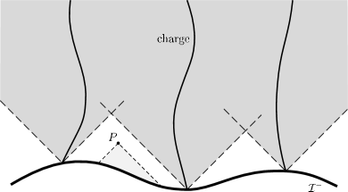
Figure 1: Fields at spacelike ${\mathcal{I}}^{-}$.

When past infinity ${\mathcal{I}}^{-}$ is spacelike, and some discrete sources “enter” the spacetime, then incoming fields must necessarily be present at ${\mathcal{I}}^{-}$ and also at such points as $P$, the past null cones of which are not crossed by the worldlines of the sources. If this is not the case, inconsistencies arise. The past null cone of $P$ is shaded in light gray, whereas the future domain of influence of sources is shaded in dark gray. (Figure taken after Penrose [9].)

One of the purposes of this paper is to study the properties of fields of pointlike sources “entering” the de Sitter universe across spacelike ${\mathcal{I}}^{-}$. We thus provide a specific physical model on which Penrose’s observation can be demonstrated and analyzed. We assume the sources and their fields to be weak enough so that they do not change the de Sitter background.

In de Sitter space we identify retarded (advanced) fields of a source as those which are in general nonvanishing only in the future (past) domain of influence of the source. As a consequence, purely retarded (advanced) fields have to vanish at the past (future) infinity. Adopting this definition we shall see that indeed purely retarded fields produced by pointlike sources cannot be smooth or even do not exist. We find this general conclusion to be true not only for charges (monopoles and dipoles) producing electromagnetic fields $(s=1)$ but, to some degree, also for scalar fields $(s=0)$ produced by scalar charges.

In general, purely retarded fields of monopoles and dipoles become singular on the past horizons (“creation light cones”) of the particle’s worldlines. A “shock-wave-type” singularity at the particle’s creation light cone can be understood similarly to a Cauchy horizon instability inside a black hole (see, e.g., Ref. [12]); an observer crossing the creation light cone sees an infinitely long history of the source in a finite interval of proper time. In the scalar field case (not considered by Penrose) no “Gaussian-type” constraints exist and retarded fields can be constructed. However, we shall see that the strength of the retarded field (the gradient of the field) of a scalar monopole has a $\delta$-function character on the creation light cone so that, for example, its energy-momentum tensor cannot be evaluated there. In the electromagnetic case it is not even possible to construct a purely retarded field of a single monopole — one has to allow additional sources on the creation light cone to find a consistent retarded solution vanishing outside the future domain of influence of the sources.

In both our somewhat different explanation of the nonexistence of purely retarded fields of general sources, and in Penrose’s original discussion, the main cause of difficulties is the spacelike character of ${\mathcal{I}}^{-}$ and the consequential existence of the past horizons, respectively, “creation light cones.”

It was only after we constructed the various types of fields produced by sources on de Sitter background and analyzed their behavior when we noticed Penrose’s general considerations in Ref. [9]. Our original motivation has been to understand fields of accelerated sources, and in particular, the electromagnetic field of uniformly accelerated charges in de Sitter spacetime. The question of electromagnetic field and its radiative properties produced by a charge with hyperbolic motion in Minkowski spacetime has perhaps been one of the most discussed “perpetual problems” of classical electrodynamics if not of all classical physics in the 20th century. Here let us only notice that the December 2000 issue of Annals of Physics contains the series of three papers (covering 80 pp.) by Eriksen and Grøn [13], which study in depth and detail various aspects of “electrodynamics of hyperbolically accelerated charges”; the papers also contain many (though not all) references on the subject.

The electromagnetic field of a uniformly accelerated charge along the $z$ axis, say, is symmetrical not only with respect to the rotations around the axis, but also with respect to the boosts along the axis. Now spacetimes with boost-rotation symmetry play an important role in full general relativity (see, e.g., Ref. [14], and references therein). They represent the only explicitly known exact solutions of the Einstein vacuum field equations, which describe moving “objects” — accelerated singularities or black holes — emitting gravitational waves, and which are asymptotically flat in the sense that they admit global, though not complete, smooth null infinity ${\mathcal{I}}^{-}$. Their radiative character is best manifested in a nonvanishing Bondi’s news function, which is an analog of the radiative part of the Poynting vector in electrodynamics. The general structure of all vacuum boost-rotation symmetric spacetimes with hypersurface orthogonal Killing vectors was analyzed in detail in Ref. [15]. One of the best known examples is the $C$-metric, describing uniformly accelerated black holes attached to conical singularities (“cosmic strings” or “struts”) along the axis of symmetry.

There exists also the generalization of the $C$-metric including a nonvanishing $\Lambda$ [16]. It has been used to study the pair creation of black holes [17]; its interpretation as uniformly accelerating black holes in a de Sitter space has been discussed recently [18]. However, no general framework is available to analyze the whole class of boost-rotation symmetric spacetimes, which are asymptotically approaching a de Sitter (or anti–de Sitter) spacetime as it is given in Ref. [15] for $\Lambda=0$. Before developing such a framework in full general relativity, we wish to gain an understanding of fields produced by (uniformly) accelerated sources in a de Sitter background. This has been our original motivation for this work.

Although it has been widely known and used in various contexts that there exists a conformal transformation between de Sitter and Minkowski spacetimes, this fact does not seem to be employed for constructing the fields of specific sources. In the following we make use of this conformal relation to find scalar and electromagnetic fields of the scalar and electric charges in de Sitter spacetime.

The plan of the paper is as follows. In Section 2, we will analyze the behavior of scalar and electromagnetic field equations with source terms under general conformal transformations. Few points contained here appear to be new, like the behavior of scalar sources in a general, $n$-dimensional spacetime, but the main purpose of this section is to review results and introduce notation needed in subsequent parts. In Section 3, the compactification of Minkowski and de Sitter spacetimes and their conformal properties are discussed. Again, all main ideas are known, especially from works of Penrose. But we need the detailed picture of the complete compactification of both spaces and explicit formulas connecting them in various coordinate systems, in order to be able to “translate” appropriate motion of the sources and their fields from Minkowski into de Sitter spacetime. The worldlines of uniformly accelerated particles in de Sitter space are defined, found, and their relation to the corresponding worldlines in Minkowski space under the conformal mapping is discussed in Section 4. In general, a single worldline in Minkowski space gets transformed into two worldlines in de Sitter space.

In Section 5, by using the conformal transformation of simple boosted spherically symmetric fields of sources in Minkowski spacetime, we construct the fields of uniformly accelerated monopole sources in de Sitter spacetime. In particular, with both the scalar and electromagnetic fields, we obtain what we call “symmetric fields.” They are analytic everywhere outside the sources and can be written as a linear combination of retarded and advanced fields from both particles. From the symmetric fields we wish to construct purely retarded fields that are nonvanishing only in the future domain of influence of particles’ worldlines. For the scalar field, this is accomplished in Section 6. We do find the retarded field, but its strength contains a $\delta$-function term located on the particle’s past horizon (creation light cone). In Section 7, the retarded electromagnetic fields are analyzed for free (unaccelerated) monopoles (Subsection A), for “rigid dipoles” (Subsection C), consisting of two close, uniformly accelerated charges of opposite sign, and for “geodesic dipoles” (Subsection D), made of two free opposite charges moving along geodesics. In Subsection B the role of the constraints, which electromagnetic fields and charges have to satisfy on any spacelike hypersurface, is emphasized. These constraints in de Sitter space with compact spatial slicings require the total charge to be zero. As is well known, there can be no net charge in a closed universe (see, e.g., Ref. [19]). However, we find out that the constraints imply even local conditions on the charge distribution if ${\mathcal{I}}^{-}$ is spacelike and purely retarded fields are only admitted. In the case of an unaccelerated electromagnetic monopole, we discover that the solution resembling retarded field represents not only the monopole charge but also a spherical shell of charges moving with the velocity of light along the creation light cone of the monopole. The total charge of the shell is precisely opposite to that of the monopole. Retarded fields of both rigid and geodesic dipoles blow up along the creation light cone since, by restricting ourselves to the fields nonvanishing in the future domain of influence, we “squeeze” the field lines produced by the dipoles into their past horizon (creation light cone).

We do not discuss the radiative character of the fields obtained. The problem of radiation is not a straightforward issue since the conformal transformation does not map an infinity onto an infinity and, thus, one has to analyze carefully the falloff (“the peeling off”) of the fields along appropriate null geodesics going to future, respectively, past spacelike infinity. A detailed discussion of the radiative properties of the solutions found here and of some additional fields will be given in a forthcoming publication [24].

A brief discussion in Section 8 concludes the paper. Some details concerning coordinate systems on de Sitter space are relegated to the Appendix.

2 Conformal invariance of scalar and electromagnetic field equations with sources

Conformal rescaling of metric is given by a common spacetime dependent conformal factor $\Omega(x)$:

$$g_{\alpha\beta}\;\;\rightarrow\;\;\hat{g}_{\alpha\beta}=\Omega^{2}g_{\alpha\beta}{\mbox{\;,\quad}}g^{\alpha\beta}\;\;\rightarrow\;\;\hat{g}^{\alpha\beta}=\Omega^{{\text{-}}2}g^{\alpha\beta}{\mbox{\;.}}$$ (2.1)

An equation for a physical field $\Psi$ is called conformally invariant if there exists a number — conformal weight — ${p\in{\mathbb{R}}}$ such that $\hat{\Psi}=\Omega^{p}\Psi$ solves a field equation with metric $\hat{g}$, if and only if $\Psi$ is a solution of the original equation with metric $g$.

It is well known (see, e.g., Ref. [20]) that (i) the wave equation for a scalar field $\Phi$ can be generalized in a conformally invariant way to curved $n$-dimensional spacetime geometry by a suitable coupling with the scalar curvature $R$, and (ii) the vacuum Maxwell’s equations are conformally invariant in four dimensions with conformal weight ${p=0}$ of covariant components (2-form) of electromagnetic field $F_{\alpha\beta}$, but they fail to be conformally invariant for dimensions $n\neq 4$.

The behavior of the above equations with sources is not so widely known (cf. Refs. [21, 10] for the electromagnetic case). It is, however, easy to see that the wave equation for the scalar field $\Phi$ with the scalar charge source $S$,

$$[\square-\xi R]\Phi=S{\mbox{\;,}}$$ (2.2)

where in $n$ dimensions $\xi=\frac{n-2}{4(n-1)}$, $R$ is the scalar curvature, and $\square=g^{\alpha\beta}\nabla_{\alpha}\nabla_{\beta}$ is the d’Alembertian constructed from the covariant metric derivative $\nabla_{\alpha}$, under the conformal rescaling Eq. (2.1) goes over into the equation of the same form

$$[\hat{\square}-\xi\hat{R}]\hat{\Phi}=\hat{S}{\mbox{\;,}}$$ (2.3)

provided that

$$\Phi\;\;\rightarrow\;\;\hat{\Phi}=\Omega^{1-\frac{n}{2}}\;\Phi{\mbox{\;,}}$$ (2.4)

$$S\;\;\rightarrow\;\;\hat{S}=\Omega^{-1-\frac{n}{2}}\;S{\mbox{\;,}}$$ (2.5)

and $\hat{\nabla}_{\alpha}$ and $\hat{R}$ are the metric covariant derivative and scalar curvature associated with the rescaled metric $\hat{g}$ (see, e.g., Eqs. (D.1)–(D.14) in Ref. [20]).

Next, it is easy to demonstrate that in four dimensions Maxwell’s equations with a source given by a four-current $J^{\alpha}$,

$$\begin{gathered}\nabla_{\mu}F^{\alpha\mu}=J^{\alpha}{\mbox{\;,}}\\ \nabla_{[\alpha}F_{\beta\gamma]}=0\quad\text{or}\quad F_{\alpha\beta}=\nabla_{\alpha}A_{\beta}-\nabla_{\beta}A_{\alpha}{\mbox{\;,}}\end{gathered}$$ (2.6)

are conformally invariant if the vector potential does not change, so that

$${\hat{A}}_{\alpha}=A_{\alpha}{\mbox{\;,\quad}}{\hat{F}}_{\alpha\beta}=F_{\alpha\beta}{\mbox{\;,\quad}}{\hat{F}}^{\alpha\beta}=\Omega^{{\text{-}}4}\,F^{\alpha\beta}{\mbox{\;,}}$$ (2.7)

and the current behaves as follows:

$${\hat{J}}^{\alpha}=\Omega^{{\text{-}}4}\,J^{\alpha}{\mbox{\;,\quad}}{\hat{J}}_{\alpha}=\Omega^{{\text{-}}2}\,J_{\alpha}{\mbox{\;.}}$$ (2.8)

Since the Levi-Civita tensor transforms as

$${\hat{\varepsilon}}_{\alpha\beta\gamma\delta}=\Omega^{4}\varepsilon_{\alpha\beta\gamma\delta}{\mbox{\;,}}$$ (2.9)

the following quantities are conformally invariant:

$${}^{*}\!{\hat{J}}_{\alpha\beta\gamma}={\hat{\varepsilon}}_{\alpha\beta\gamma\mu}{\hat{J}}^{\mu}={}^{*}\!J_{\alpha\beta\gamma}{\mbox{\;,}}$$ (2.10)

$${}^{*}\!{\hat{F}}_{\alpha\beta}=\frac{1}{2!}{\hat{\varepsilon}}_{\alpha\beta\mu\nu}{\hat{F}}^{\mu\nu}={}^{*}\!F_{\alpha\beta}{\mbox{\;.}}$$ (2.11)

Therefore, Maxwell’s equations with a source can be written using the external derivative as

$$\mathrm{d}F=0{\mbox{\;,\quad}}\mathrm{d}{}^{*}\!F=-2\,{}^{*}\!J{\mbox{\;,}}$$ (2.12)

where only conformally invariant quantities appear.

The continuity equation for the electromagnetic current is also conformally invariant:

$$\nabla_{\alpha}J^{\alpha}=0\;\;\rightarrow\;\;{\hat{\nabla}}_{\alpha}{\hat{J}}^{\alpha}=\Omega^{{\text{-}}4}\nabla_{\alpha}J^{\alpha}=0$$ (2.13)

thanks to Eq. (2.8) and the conformal property of the four-dimensional volume element ${{\mathfrak{g}}^{1/2}}=(-\operatorname{Det}g_{\alpha\beta})^{1/2}$:

$${\hat{\mathfrak{g}}}^{1/2}=\Omega^{4}{{\mathfrak{g}}^{1/2}}{\mbox{\;.}}$$ (2.14)

It is interesting to notice, however, that as a consequence of the invariance (2.7) of the electromagnetic potential under a conformal rescaling, the Lorentz gauge condition is not conformally invariant:

$$\nabla_{\alpha}A^{\alpha}=0$$ (2.15)

implies

$${\hat{\nabla}}_{\alpha}{\hat{A}}^{\alpha}-2{\hat{A}}^{\alpha}\,\mathrm{d}_{\alpha}\log\left\lvert\Omega\right\rvert=0{\mbox{\;.}}$$ (2.16)

A remarkable property arises in four-dimensional spacetimes: in both the scalar and electromagnetic case the total charge distributed on a three-dimensional spacelike hypersurface is conformally (pseudo)invariant. This follows form the conformal invariance of spatial charge distributions.

Denoting $n_{\alpha}$ a future-oriented unit 1-form normal to the hypersurface $\Sigma$, we get

$${\hat{n}}_{\alpha}=\left\lvert\Omega\right\rvert n_{\alpha}{\mbox{\;,\quad}}{\hat{n}}^{\alpha}=\left\lvert\Omega\right\rvert^{-1}n^{\alpha}{\mbox{\;.}}$$ (2.17)

The three-dimensional volume element is given by ${{\mathfrak{q}}^{1/2}}=(\operatorname{Det}q_{\alpha\beta})^{1/2}$, where three-metric $q_{\alpha\beta}$ is the restriction of the four-metric $g_{\alpha\beta}$ to the hypersurface $\Sigma$. Under the conformal transformation,

$${{\mathfrak{q}}^{1/2}}\;\;\rightarrow\;\;{\hat{\mathfrak{q}}}{}^{1/2}=\left\lvert\Omega\right\rvert^{3}{{\mathfrak{q}}^{1/2}}{\mbox{\;.}}$$ (2.18)

A charge distribution is defined as a charge density multiplied by this volume element. Hence, the scalar charge distribution reads

$$\sigma=S\,{{\mathfrak{q}}^{1/2}}{\mbox{\;,}}$$ (2.19)

and

$$\sigma\;\;\rightarrow\;\;\hat{\sigma}=\operatorname{sign}(\Omega)\;\sigma{\mbox{\;.}}$$ (2.20)

We see that it is conformal invariant except for a change of sign if the conformal factor $\Omega$ is negative. As seen from Eq. (2.5), this fails to be true for $n\neq 4$. In the following we consider only the case $n=4$.

The electromagnetic charge distribution is given by

$$\rho=n_{\alpha}J^{\alpha}\;{{\mathfrak{q}}^{1/2}}{\mbox{\;.}}$$ (2.21)

Again, regarding Eqs. (2.8), (2.17), and (2.18), we get

$$\rho\;\;\rightarrow\;\;\hat{\rho}=\rho{\mbox{\;.}}$$ (2.22)

Thus, the electromagnetic charge is invariant even under conformal transformation with a negative conformal factor $\Omega$.

Similarly, we define the electric field with the three-dimensional volume element included:

$${\mathcal{E}}^{\alpha}=n_{\mu}F^{\mu\alpha}\;{{\mathfrak{q}}^{1/2}}{\mbox{\;,}}$$ (2.23)

which represents the momentum conjugated to the potential $A_{\alpha}$ (cf., e.g., Ref. [19]). With the definition (2.23), ${\mathcal{E}}^{\alpha}$ is conformally invariant. Gauss’s law simply reads

$$\int_{D}\nabla^{\scriptscriptstyle{(3)}}_{\alpha}{\mathcal{E}}^{\alpha}=\int_{\partial{D}}{\mathcal{E}}^{\alpha}dS_{\alpha}{\mbox{\;,}}$$ (2.24)

where $\nabla^{\scriptscriptstyle{(3)}}$ is three-metric covariant derivative and $D$ is a region in $\Sigma$.

3 Minkowski and de Sitter spacetimes:
compactification and conformal relation

The conformal structure of Minkowski and de Sitter spacetimes and their conformal relation to the regions of the Einstein static universe is well known and has been much used (see, e.g., Refs. [6, 20] for basic expositions). However, the complete compactified picture of both spaces and their conformal structure do not appear to be described in detail in the literature, although all main ideas are contained in various writings by Penrose (e.g. Refs. [9, 10]). Since we shall need some details in explicit form when analyzing the character of the fields of sources in de Sitter spacetime and their relation to their counterparts in Minkowski spacetime, we shall now discuss the compactification and conformal properties of these spaces.

Recall first that flat Euclidean plane $E^{2}$ can be compactified by adding a point at infinity so that the resulting space is a two-sphere $S^{2}$ with a regular homogenous metric $g_{{\scriptscriptstyle{\mathrm{sph}}}}$, conformally related to the Euclidean metric:

$$g_{\scriptscriptstyle{\mathrm{sph}}}=\alpha^{2}\bigl{(}\mathrm{d}\vartheta{}^{\,2}+\sin^{2}\!\vartheta\,\mathrm{d}\varphi{}^{\,2}\bigr{)}=\Omega^{2}\bigl{(}\mathrm{d}r{}^{\,2}+r^{2}\mathrm{d}\varphi{}^{\,2}\bigr{)}=\Omega^{2}g_{\scriptscriptstyle{\mathrm{Eucl}}}{\mbox{\;,}}$$ (3.25)

where $\alpha$ is a constant parameter with the dimension of length, $r=\alpha\tan\frac{\vartheta}{2}$, and $\Omega=1+\cos\vartheta$. Notice that $g_{\scriptscriptstyle{\mathrm{Eucl}}}$ is not regular at $r=\infty$, where the conformal factor $\Omega=0$. The group of conformal transformations of $E^{2}$ acts on the compact manifold $S^{2}$.

Analogously, one can construct compactified Minkowski space $M^{\#}$ (see Ref. [10], Section 9.2 and references therein) on which the 15-parameter conformal group acts. One starts with the standard Penrose diagram of Minkowski space and makes an identification of ${\mathcal{I}}_{\scriptscriptstyle{\mathrm{Mink}}}^{-}$ and ${\mathcal{I}}_{\scriptscriptstyle{\mathrm{Mink}}}^{+}$ by identifying the past and future endpoints of null geodesics as indicated in Fig. 2. The future and past timelike infinities, $i_{\scriptscriptstyle{\mathrm{Mink}}}^{\pm}$, and the spatial infinity, $i_{\scriptscriptstyle{\mathrm{Mink}}}^{0}$, are also identified into one point. The topology of $M^{\#}$ is $S^{3}\times S^{1}$ (this is not evident from first sight, but see Ref. [10]).

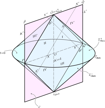
Figure 2: Three-dimensional Penrose diagram of Minkowski space

The whole spacetime is mapped into the interior of two cones joined base to base along a spacelike (Cauchy) hypersurface $t=0$. The boundary of the two cones consists of past and future null infinities, ${\mathcal{I}}_{\scriptscriptstyle{\mathrm{Mink}}}^{-}$, ${\mathcal{I}}_{\scriptscriptstyle{\mathrm{Mink}}}^{+}$, of the past and future timelike infinities, $i_{\scriptscriptstyle{\mathrm{Mink}}}^{-}$, $i_{\scriptscriptstyle{\mathrm{Mink}}}^{+}$, and of the spacelike infinity, $i_{\scriptscriptstyle{\mathrm{Mink}}}^{0}$. At these infinities, the null, timelike, and spacelike geodesics start and end. A two-dimensional cut $\mathcal{C}$ going through $i_{\scriptscriptstyle{\mathrm{Mink}}}^{-}$, $i_{\scriptscriptstyle{\mathrm{Mink}}}^{+}$, and $P,Q\in i_{\scriptscriptstyle{\mathrm{Mink}}}^{0}$ is considered, with two null geodesics $A^{\prime}XA$ and $B^{\prime}YB$ indicated. It is divided into four separate regions, I–IV. Regions III and IV are mapped into regions III’ and IV’ in the compactified Minkowski space illustrated in Fig. 3.

Rescaled Minkowski space (without the identification) can be drawn in a two-dimensional diagram as a part of the Einstein static universe, which is visualized by a cylindrical surface imbedded in $E^{3}$ — see, e.g., Refs. [6, 20]. However, in Fig. 3 we illustrate the compactified Minkowski space $M^{\#}$ by a three-dimensional diagram as a part of the Einstein universe represented by a solid cylinder in $E^{3}$. This is achieved in the following way: In Fig. 2 the Minkowski spacetime (with one dimension suppressed) is illustrated as a region bounded by two cones joined base to base. Now we take a two-dimensional cut $\mathcal{C}$ and we compactify it by dividing it into four regions, I–IV, as indicated in Fig. 2. We cut out regions III and IV and place them “above” regions II and I so that they are joined along their corresponding null boundaries (e.g., points $B$, $B^{\prime}$ and $A$, $A^{\prime}$ become identical). Now the segment $PO$ has to be identified with $\tilde{O}\tilde{Q}$ and $OQ$ with $\tilde{P}\tilde{O}$ — they correspond to a single segment in Fig. 2. Similarly, boundaries $P\tilde{P}$ and $Q\tilde{Q}$ are identified, and as a result a compact manifold is formed. Consider then all posible cuts $\mathcal{C}$, i.e., “rotate” $\mathcal{C}$ around the “line” $i_{\scriptscriptstyle{\mathrm{Mink}}}^{-}Oi_{\scriptscriptstyle{\mathrm{Mink}}}^{+}$, and make the same identifications as we just described. Now all “vertical” boundary lines as $P\tilde{P}$ and $Q\tilde{Q}$ have to be identified (notice that all these points were on the segment $i_{\scriptscriptstyle{\mathrm{Mink}}}^{-}O$ in Fig. 2). The resulting four-dimensional compact manifold is represented in the three-dimensional Fig. 3. From the construction described, it follows that the top and bottom bases of the solid cylinder are identified and each of the circles on the cylindrical surface, as, e.g., $k$, should be considered as a single point. The “disks” inside these circles are thus two-spheres, i.e., without suppressing one dimension — three-spheres in $M^{\#}$.

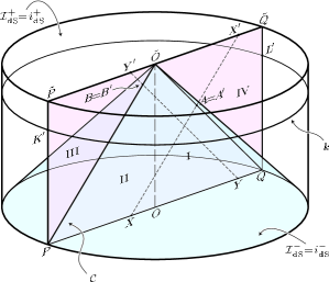
Figure 3: Compactified Minkowski and de Sitter spaces

The compactified Minkowski and de Sitter space $M^{\#}$, illustrated by the three-dimensional diagram — a part of the Einstein universe represented here as a solid cylinder. The compactification is achieved by considering first the two-dimensional section $\mathcal{C}$ in Fig. 2, cutting out regions III and IV and placing them “above” regions II and I so that two-dimensional figure $POQ\tilde{Q}\tilde{O}\tilde{P}$ is formed. $PO$ is identified with $\tilde{O}\tilde{Q}$ (e.g., point $X$ with $X^{\prime}$), $OQ$ with $\tilde{P}\tilde{O}$ (e.g., $Y$ with $Y^{\prime}$), and $P\tilde{P}$ with $Q\tilde{Q}$. All two-dimensional cuts $\mathcal{C}$ are identified in this way with, in addition, all “vertical” boundary lines being identified so that the circle $k$, for example, is considered as a point. The top and bottom bases of the cylinder, representing the past and the future spacelike infinities of de Sitter space, are identified in the compact manifold $M^{\#}$.

Now it is important to realize that Fig. 3 can be understood as a part of the Einstein static cylinder, which also represents the compactified de Sitter space. In de Sitter space two bases are future and past spacelike infinities. They are not usually identified in the standard two-dimensional Penrose diagram of de Sitter spacetime (see, e.g., Ref. [6]), as ${\mathcal{I}}_{\scriptscriptstyle{\mathrm{Mink}}}^{+}$ and ${\mathcal{I}}_{\scriptscriptstyle{\mathrm{Mink}}}^{-}$ are not identified in the standard Penrose diagram of Minkowski space.

Manifold $M^{\#}$ represents the compactification of both Minkowski and de Sitter space. Similarly as $S^{2}$, representing the compactification of $E^{2}$, can be equipped with a regular metric $g_{\scriptscriptstyle{\mathrm{sph}}}$ mentioned above, $M^{\#}$ can be equipped with the regular metric

$$g_{\scriptscriptstyle{\mathrm{Eins}}}=\alpha^{2}\;\bigl{(}-\mathrm{d}{\tilde{t}}{}^{\,2}+\mathrm{d}{\tilde{r}}{}^{\,2}+\sin^{2}\!{\tilde{r}}\;{\mathrm{d}\omega^{2}}\bigr{)}{\mbox{\;,}}$$ (3.26)

where dimensionless coordinates ${\tilde{t}},{\tilde{r}}\in\langle 0,\pi\rangle$, spacelike hypersufaces ${\tilde{t}}=0$, and ${\tilde{t}}=\pi$ are identified by means of null geodesics, ${\mathrm{d}\omega^{2}}=\mathrm{d}\vartheta{}^{\,2}+\sin^{2}\!\vartheta\,\mathrm{d}\varphi{}^{\,2}$, and the constant $\alpha$ has dimension of length. The metric (3.26) is the well known metric of the Einstein universe, in which case

$$\alpha^{2}=\frac{3}{\Lambda}{\mbox{\;,}}$$ (3.27)

where $\Lambda$ is the cosmological constant.

In order to see this explicitly, write the Minkowski metric in standard spherical coordinates,

$$g_{\scriptscriptstyle{\mathrm{Mink}}}=-\mathrm{d}t{}^{\,2}+\mathrm{d}r{}^{\,2}+r^{2}\,{\mathrm{d}\omega^{2}}{\mbox{\;,}}$$ (3.28)

and introduce coordinates ${\tilde{t}},{\tilde{r}}\in\langle 0,\pi\rangle$ by

$${\tilde{t}}=\arctan\frac{2\alpha t}{\alpha^{2}-t^{2}+r^{2}}{\mbox{\;,\quad}}{\tilde{r}}=\arctan\frac{2\alpha r}{\alpha^{2}+t^{2}-r^{2}}{\mbox{\;,}}$$ (3.29)

inversely

$$t=\frac{\alpha\sin{\tilde{t}}}{\cos{\tilde{r}}+\cos{\tilde{t}}}{\mbox{\;,\quad}}r=\frac{\alpha\sin{\tilde{r}}}{\cos{\tilde{r}}+\cos{\tilde{t}}}{\mbox{\;,}}$$ (3.30)

so that

$$g_{\scriptscriptstyle{\mathrm{Mink}}}=\frac{\alpha^{2}}{(\cos{\tilde{r}}+\cos{\tilde{t}})^{2}}\;\bigl{(}-\mathrm{d}{\tilde{t}}{}^{\,2}+\mathrm{d}{\tilde{r}}{}^{\,2}+\sin^{2}\!{\tilde{r}}\;{\mathrm{d}\omega^{2}}\bigr{)}{\mbox{\;.}}$$ (3.31)

Let us notice that by requiring the ranges ${\tilde{t}},{\tilde{r}}\in\langle 0,\pi\rangle$, we fix the branch of $\arctan$ in Eq. (3.29). Further, observe that for ${\tilde{t}}+{\tilde{r}}>\pi$, relations (3.30) imply negative $r$ — we shall return to this point in a moment.

In the case of de Sitter space with the metric

$$g_{\scriptscriptstyle{\mathrm{dS}}}=-\mathrm{d}\tau{}^{\,2}+\alpha^{2}\cosh^{2}\!\frac{\tau}{\alpha}\;\Bigl{(}\mathrm{d}\chi{}^{\,2}+\sin^{2}\!\chi\;{\mathrm{d}\omega^{2}}\Bigr{)}{\mbox{\;,}}$$ (3.32)

we put

$${\tilde{t}}=2\arctan\Bigl{(}\exp\frac{\tau}{\alpha}\,\Bigr{)}{\mbox{\;,\quad}}{\tilde{r}}=\chi{\mbox{\;,}}$$ (3.33)

or

$$\tau=\alpha\log\Bigl{(}\tan\frac{{\tilde{t}}}{2}\,\Bigr{)}{\mbox{\;,\quad}}\chi={\tilde{r}}{\mbox{\;,}}$$ (3.34)

so that

$$g_{\scriptscriptstyle{\mathrm{dS}}}=\frac{\alpha^{2}}{\sin^{2}{\tilde{t}}}\;\bigl{(}-\mathrm{d}{\tilde{t}}{}^{\,2}+\mathrm{d}{\tilde{r}}{}^{\,2}+\sin^{2}\!{\tilde{r}}\;{\mathrm{d}\omega^{2}}\bigr{)}{\mbox{\;.}}$$ (3.35)

In this way we obtain explicit forms of the conformal rescaling of both spaces into the metric of the Einstein universe:

$$g_{\scriptscriptstyle{\mathrm{Eins}}} =\Omega_{\scriptscriptstyle{\mathrm{Mink}}}^{2}\;g_{\scriptscriptstyle{\mathrm{Mink}}}{\mbox{\;,\quad}} \Omega_{\scriptscriptstyle{\mathrm{Mink}}}=\cos{\tilde{r}}+\cos{\tilde{t}}{\mbox{\;,}}$$ (3.36)

$$g_{\scriptscriptstyle{\mathrm{Eins}}} =\Omega_{\scriptscriptstyle{\mathrm{dS}}}^{2}\;g_{\scriptscriptstyle{\mathrm{dS}}}{\mbox{\;,\quad}} \Omega_{\scriptscriptstyle{\mathrm{dS}}}=\sin{\tilde{t}}{\mbox{\;,}}$$ (3.37)

where $g_{\scriptscriptstyle{\mathrm{Eins}}}$ is given by Eq. (3.26). As in the simple case of conformal relation of $E^{2}$ to $S^{2}$, the conformal factors $\Omega_{\scriptscriptstyle{\mathrm{Mink}}}$ and $\Omega_{\scriptscriptstyle{\mathrm{dS}}}$ vanish at infinities of Minkowski, respectively, de Sitter space.

As a consequence of Eqs. (3.29)–(3.35) we also find the conformal relation between Minkowski and de Sitter space:

$$g_{\scriptscriptstyle{\mathrm{Mink}}}=\Omega^{2}g_{\scriptscriptstyle{\mathrm{dS}}}{\mbox{\;,\quad}}\Omega=\Omega_{\scriptscriptstyle{\mathrm{Mink}}}^{{\text{-}}1}\,\Omega_{\scriptscriptstyle{\mathrm{dS}}}{\mbox{\;,}}$$ (3.38)

where $\Omega_{\scriptscriptstyle{\mathrm{Mink}}}$, $\Omega_{\scriptscriptstyle{\mathrm{dS}}}$ are given by Eqs. (3.36) and (3.37). The conformal factor $\Omega$ has the simplest form when expressed in terms of the Minkowski time $t$:

$$\Omega=\frac{\sin{\tilde{t}}}{\cos{\tilde{r}}+\cos{\tilde{t}}}=\frac{t}{\alpha}{\mbox{\;.}}$$ (3.39)

The conformal transformation is not regular at the infinity of Minkowski, respectively, de Sitter space because $\Omega$ diverges, respectively, vanishes there. We shall return to this point at the end of this section. First, however, we have to describe the coordinate systems employed in relating particular regions I–IV in Figs. 2 and 3.

Relations (3.29) and (3.30) can be used automatically in region I only. In other regions, ranges of coordinates have to be specified more carefully. In the following we always require ${\tilde{t}}\in\langle 0,\pi\rangle$. Then, if ${\tilde{r}}\in\langle 0,\pi\rangle$, we find that relations (3.29) and (3.30) imply negative $r$ in region IV. Also, if we consider events with $t<0$, $r>0$ (region III), we notice that as a consequence of Eqs. (3.29) and (3.30) with ${\tilde{t}}\in\langle 0,\pi\rangle$ we get ${\tilde{r}}<0$. Relations (3.29) and (3.30) can be made meaningful in all regions I–IV if we allow negative $r$, ${\tilde{r}}$ and adopt the following convention: at a fixed value of time coordinate $t$, respectively, ${\tilde{t}}$, the points symmetrical with respect to the origin of spherical coordinates have opposite signs of the radial coordinate, i.e., points with given $\{t,r,\vartheta,\varphi\}$, respectively $\{{\tilde{t}},{\tilde{r}},\vartheta,\varphi\}$, are identical with $\{t,-r,\pi-\vartheta,\varphi+\pi\}$, respectively $\{{\tilde{t}},-{\tilde{r}},\pi-\vartheta,\varphi+\pi\}$. The way in which regions I–IV are covered by the particular ranges of coordinates is explicitly illustrated in Figs. 5(a)–5(c) in the Appendix, where our convention is described in more detail.

In the Appendix, various useful coordinate systems in de Sitter space are given. First, we shall frequently employ coordinates $\{{\tilde{t}},{\tilde{r}},\vartheta,\varphi\}$ which are simply related (by Eqs. (3.33) and (3.34)) to the standard coordinates $\{\tau$, $\chi$, $\vartheta$, $\varphi\}$ covering nicely the whole de Sitter hyperboloid. Next, relations (3.29) and (3.30) can be viewed as the definition of another coordinate system $\{t,r,\vartheta,\varphi\}$ on de Sitter space (with the metric being given by Eq. (A.92)). Let us remind that for fixed $\vartheta$, $\varphi$ values ${\tilde{r}}>0$ (commonly assumed in de Sitter space) correspond to $r>0$ for ${\tilde{t}}+{\tilde{r}}<\pi$ (region I) and to $r<0$ for ${\tilde{t}}+{\tilde{r}}>\pi$ (region IV). Further, one frequently uses static coordinates $T$, $R$ associated with the static Killing vector of de Sitter spacetime — Eqs. (A.94) in the Appendix.

Finally, it will be useful to introduce the null coordinates (cf. Eq. (A.98))

$$u=t-r{\mbox{\;,\quad}}v=t+r{\mbox{\;,}}$$ (3.40)

$${\tilde{u}}={\tilde{t}}-{\tilde{r}}{\mbox{\;,\quad}}{\tilde{v}}={\tilde{t}}+{\tilde{r}}{\mbox{\;.}}$$ (3.41)

When employing null coordinates we shall consider only ${\tilde{r}}>0$ (${\tilde{u}}$, ${\tilde{v}}$ would “exchange their role” if ${\tilde{r}}<0$); the ranges of ${\tilde{u}},{\tilde{v}}$ and $u,v$ are thus given by the choice ${\tilde{t}},{\tilde{r}}\in\langle 0,\pi\rangle$. This leaves the standard (Minkowski) meaning of $u$, $v$ in region I; however, $u$ and $v$ exchange their usual (Minkowski) role in region IV (${\tilde{v}}={\tilde{t}}+{\tilde{r}}>\pi$) because here $r<0$. With this choice, the coordinates ${\tilde{u}}$, ${\tilde{v}}$ and $u$ cover de Sitter space continuously, in particular the horizon ${\tilde{v}}=\pi$ ($v\rightarrow\pm\infty$ on this horizon — see Fig. 5(e)).

From Eqs. (3.29) and (3.30) we get simple relations

$$u=\alpha\tan\frac{{\tilde{u}}}{2}{\mbox{\;,\quad}}v=\alpha\tan\frac{{\tilde{v}}}{2}{\mbox{\;,}}$$ (3.42)

which explicitly verify that local null cones (local causal structure) are unchanged under conformal mapping. Nevertheless, it is well known that the global causal structure of the Minkowski and de Sitter space is different. This is reflected in the fact that, as mentioned above, the conformal transformation between the two spaces is not regular everywhere. In particular, relation (3.42) shows that points at null infinity with $v\rightarrow\pm\infty$ in Minkowski space go over into regular points with ${\tilde{v}}\rightarrow\pi$ in de Sitter space, whereas spacelike hypersurface $t=\frac{1}{2}(u+v)=0$ goes into spacelike infinities ${\tilde{t}}=0,\pi$ in de Sitter space.

In the next sections, when we shall generate solutions for the scalar and electromagnetic fields for given sources in de Sitter space by employing the conformal transformation from Minkowski space, we have to check the behavior of the new solutions at points where the transformation is not regular.

Before turning to the construction of the fields produced by specific sources, let us emphasize that in all the following expressions for fields in de Sitter spacetime only positive ${\tilde{r}}$ can be considered. However, the results contained in Sections 4 and 5 are valid also for ${\tilde{r}}<0$ provided that the convention described above is used.

4 Uniformly accelerated particles in de Sitter spacetime

In this section we study the correspondence of the worldlines of uniformly accelerated particles under the conformal mapping (3.29) and (3.30) between Minkowski and de Sitter spacetimes. Let a particle have four-velocity $u^{\alpha}$, ${u^{\mu}u_{\mu}=-1}$, so that its acceleration is $a^{\alpha}=\dot{u}^{\alpha}=u^{\mu}\nabla_{\mu}u^{\alpha}$, $a^{\mu}u_{\mu}=0$. We say that the particle is uniformly accelerated if the projection of $\dot{a}^{\alpha}=u^{\mu}\nabla_{\mu}a^{\alpha}$ into the three-surface orthogonal to $u^{\alpha}$ vanishes:

$$P^{\alpha}_{\mu}\,\dot{a}^{\mu}=\dot{a}^{\alpha}-(a^{\mu}a_{\mu})\,u^{\alpha}=0{\mbox{\;.}}$$ (4.43)

Here the projection tensor $P^{\mu}_{\nu}=\delta^{\mu}_{\nu}+u^{\mu}u_{\nu}$ and $u_{\mu}\dot{a}^{\mu}=-a_{\mu}a^{\mu}$. Multiplying Eq. (4.43) by $a^{\alpha}$, we get $\dot{a}^{\mu}a_{\mu}=0$ so that

$$a_{\mu}a^{\mu}=\text{constant}{\mbox{\;.}}$$ (4.44)

This definition of uniform acceleration goes over into the standard definition used in Minkowski space [22]. It implies that the components of a particle’s acceleration in its instantaneous rest frames remain constant. Of course, as a special case, a particle may have zero acceleration when it moves along the geodesic.

Consider a particle moving with a constant velocity

$$\frac{R_{\mathrm{o}}}{\alpha}=\tanh\beta=\text{constant}$$ (4.45)

along the $z$ axis ($\varphi=0$, $\vartheta=0$) of the inertial frame in Minkowski spacetime with coordinates $\{t,r,\vartheta,\varphi\}$ so that it passes through $r=0$ at $t=0$. Transformations (3.29), (3.30) map its worldline into two worldlines in de Sitter spacetime, given in terms of parameter $\lambda_{\scriptscriptstyle{\mathrm{Mink}}}$, its proper time in Minkowski space, or in terms of $\lambda_{\scriptscriptstyle{\mathrm{dS}}}$, its proper time in de Sitter space, as follows:

$$\begin{gathered}{\tilde{t}}=\arctan\Bigl{(}-2\alpha\,\frac{\lambda_{\scriptscriptstyle{\mathrm{Mink}}}\cosh\beta}{\lambda_{\scriptscriptstyle{\mathrm{Mink}}}^{2}-\alpha^{2}}\Bigr{)}=\arctan\Bigl{(}-\frac{\cosh\beta}{\sinh\bigl{(}({\lambda_{\scriptscriptstyle{\mathrm{dS}}}}/{\alpha})\cosh\beta\bigr{)}}\Bigr{)}{\mbox{\;,}}\\ {\tilde{r}}=\arctan\Bigl{(}2\alpha\,\frac{\lambda_{\scriptscriptstyle{\mathrm{Mink}}}\sinh\beta}{\lambda_{\scriptscriptstyle{\mathrm{Mink}}}^{2}+\alpha^{2}}\Bigr{)}=\arctan\Bigl{(}\pm\frac{\sinh\beta}{\cosh\bigl{(}({\lambda_{\scriptscriptstyle{\mathrm{dS}}}}/{\alpha})\cosh\beta\bigr{)}}\Bigr{)}{\mbox{\;.}}\end{gathered}$$ (4.46)

In these expressions, the $\arctan$ has values in $\langle 0,\pi\rangle$; $\lambda_{\scriptscriptstyle{\mathrm{dS}}}\in{\mathbb{R}}$, and $\lambda_{\scriptscriptstyle{\mathrm{Mink}}}\in(0,\infty)$ for the worldline starting and ending with ${\tilde{r}}=0$ (denoted by $1$ in Fig. 4; plus sign in the last equation in (4.46)), whereas $\lambda_{\scriptscriptstyle{\mathrm{Mink}}}\in(-\infty,0)$ for the second worldline, starting and ending with ${\tilde{r}}=\pi$ (denoted by $1^{\prime}$ in Fig. 4; minus sign in (4.46)). One thus gets two worldlines in de Sitter space from two “halves” of one worldline in Minkowski space.

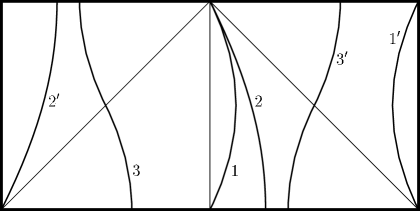
Figure 4: Worldlines of particles in de Sitter spacetime

The worldlines of geodesics and of uniformly accelerated particles in de Sitter spacetime, obtained by the conformal transformation of appropriate worldlines in Minkowski space: $1$, $1^{\prime}$ from the worldline of a particle moving uniformly through the origin, $2$, $2^{\prime}$ from a particle at rest outside the origin, and $3$, $3^{\prime}$ from two uniformly accelerated particles. In de Sitter space, the worldlines $1$ and $1^{\prime}$ describe two uniformly accelerated particles; $2$, $2^{\prime}$ and $3$, $3^{\prime}$ are geodesics. Both particles in each pair are causally disconnected.

These two worldlines are uniformly accelerated with the constant magnitude of the acceleration equal (up to the sign) to

$$a_{\mathrm{o}}=-\frac{1}{\alpha}\sinh\beta{\mbox{\;.}}$$ (4.47)

An intuitive understanding of the acceleration is gained if we introduce standard static coordinates $\{T,R,\vartheta,\varphi\}$ in de Sitter space (see the Appendix). The two worldlines described by Eq. (4.46) in coordinates ${\tilde{t}},{\tilde{r}}$ are in the static coordinates simply given by $R=R_{\mathrm{o}}=\text{constant}$. (As seen from Eq. (A.94), for a given ${\tilde{t}}$, ${\tilde{r}}$, the same $R$ corresponds to ${\tilde{r}}$ and $\pi-{\tilde{r}}$.) Owing to the “cosmic repulsion” caused by the presence of a cosmological constant, fundamental geodesic observers with fixed ${\tilde{r}}$ (i.e., fixed $\chi$) are “repelled” one from the other in proportion to their distance. Their initial implosion starting at ${\tilde{t}}=0$ ($\tau=-\infty$) is stopped at ${\tilde{t}}=\pi/2$ ($\tau=0$ — at the “neck” of the de Sitter hyperboloid) and changes into expansion. A particle having constant $R=R_{\mathrm{o}}$, thus a constant proper distance from an observer at ${\tilde{r}}=R=0$ (or at ${\tilde{r}}=\pi$, $R=0$), has to be accelerated towards that observer. The acceleration of particle $1$ points towards the observer at ${\tilde{r}}=0$, whereas that of particle $1^{\prime}$ points towards the observer at ${\tilde{r}}=\pi$ (Fig. 4). Notice that the two uniformly accelerated worldlines are causally disconnected; no retarded or advanced effects from the particle $1$ can reach the particle $1^{\prime}$ and vice versa. This is analogous to two particles symmetrically located along opposite parts of say the $z$ axis and uniformly accelerated in opposite directions in Minkowski space. The worldlines of uniformly accelerated particles in Minkowski space are the orbits of the boost Killing vector. Analogously, in de Sitter space the Killing vector ${\frac{\partial}{\partial T}}$ also has the character of a boost.

Another type of simple worldline in de Sitter space arises from transforming the worldlines of a particle at rest at $r=r_{\mathrm{o}}$ ($\left\lvert r_{\mathrm{o}}\right\rvert<\alpha$), $\vartheta=0$, $\varphi=0$ in Minkowski space. It transforms to two worldlines in de Sitter space given by

$$\begin{gathered}{\tilde{t}}=\arctan\Bigl{(}\frac{2\alpha\lambda_{\scriptscriptstyle{\mathrm{Mink}}}}{-\lambda_{\scriptscriptstyle{\mathrm{Mink}}}^{2}+r_{\mathrm{o}}^{2}+\alpha^{2}}\Bigr{)}{\mbox{\;,}}\\ {\tilde{r}}=\arctan\Bigl{(}\frac{-2\alpha r_{\mathrm{o}}}{-\lambda_{\scriptscriptstyle{\mathrm{Mink}}}^{2}+r_{\mathrm{o}}^{2}-\alpha^{2}}\Bigr{)}{\mbox{\;,}}\\ \vartheta=0{\mbox{\;,\quad}}\varphi=0{\mbox{\;,}}\end{gathered}$$ (4.48)

with ${\tilde{t}}\in\langle 0,\pi\rangle$, and ${\tilde{r}}\,\operatorname{sign}r_{\mathrm{o}}\in\langle 0,\pi\rangle$ for $\lambda_{\scriptscriptstyle{\mathrm{Mink}}}>0$ and ${\tilde{r}}\,\operatorname{sign}r_{\mathrm{o}}\in\langle-\pi,0\rangle$ for $\lambda_{\scriptscriptstyle{\mathrm{Mink}}}<0$. Thus, a geodesic in Minkowski space goes over into two geodesics in de Sitter space. In Fig. 4 these are the worldlines $2$ and $2^{\prime}$.

As the last example, let us just mention that the worldlines of two particles uniformly accelerated in Minkowski space get transformed into two geodesics $3$, $3^{\prime}$ in de Sitter space.

5 Scalar and electromagnetic fields from uniformly accelerated particles: the symmetric solutions

Two uniformly accelerated particles described by worldlines (4.46) were obtained by the conformal transformation from the worldline of a particle moving with a uniform velocity ${R_{\mathrm{o}}}/{\alpha}$ in Minkowski space. Hence, their fields can be constructed by the conformal transformation of a simple boosted spherically symmetric field. In the case of scalar field, Eqs. (2.4), (2.20), and (3.39) then lead to the field

$$\Phi=\frac{s}{4\pi}\frac{t}{\alpha}\,\frac{1}{\left\lvert r^{\prime}\right\rvert}{\mbox{\;,}}$$ (5.49)

where $r^{\prime}$ is spherical coordinate in an inertial frame in which the particle is at rest at the origin.

As emphasized earlier, we have to examine the field at the null hypersurface ${\tilde{v}}=\pi$, where the conformal transformation fails to be regular. We find that field (5.49) is indeed not smooth there. The limit of $\Phi$ as ${\tilde{v}}=\pi$ is approached from the region ${\tilde{v}}<\pi$ differs from the limit from ${\tilde{v}}>\pi$; $\Phi$ has a jump at ${\tilde{v}}=\pi$, although, as can be checked by a direct calculation, this discontinuous field satisfies the scalar wave equation. However, a field analytic everywhere outside the sources can be obtained by an analytic continuation of the field (5.49) from the domain ${\tilde{v}}<\pi$ to the domain ${\tilde{v}}>\pi$. We discover that the new field in ${\tilde{v}}>\pi$ differs from Eq. (5.49) just by a sign. Therefore it simply corresponds to the charge of the particle in ${\tilde{v}}>\pi$, which is opposite to that implied by conformal transformation. It is easy to see that, due to the conformal transformation, the sign of the charge on the worldline with ${\tilde{v}}>\pi$ is opposite to the original charge $s$ because the conformal factor $\Omega=t/\alpha<0$ for ${\tilde{v}}>\pi$. Hence, the field which is analytic represents the field of two uniformly accelerated particles with the same scalar charge $s$, which move along two worldlines given by (4.46). In Section 6 we shall see that this field can be written as a linear combination of retarded and advanced fields from both particles. We call it the symmetric field. Regarding Eq. (5.49), in which $r^{\prime}$ is first expressed in terms of the original Minkowski coordinates $\{t,r,\vartheta,\varphi\}$, and then using the transformation (3.30), we find the field as a function of $\{{\tilde{t}},{\tilde{r}},\vartheta,\varphi\}$:

$$\Phi_{\mathrm{sym}}=\frac{s}{4\pi}\frac{\sqrt{\alpha^{2}-R_{\mathrm{o}}^{2}}}{\sqrt{(\alpha^{2}-RR_{\mathrm{o}}\cos\vartheta)^{2}-(\alpha^{2}-R^{2})(\alpha^{2}-R_{\mathrm{o}}^{2})}}{\mbox{\;,}}$$ (5.50)

where $R=\alpha\frac{\sin{\tilde{r}}}{\sin{\tilde{t}}}$ is the static radial de Sitter coordinate (see the Appendix). As could have been anticipated, the field is static in the static coordinates since the accelerated particles are at rest at $R=R_{\mathrm{o}}$, $\vartheta=\varphi=0$. (Recall that we need two sets of such coordinates to cover both worldlines but the coordinate $R$ is well defined in the whole de Sitter spacetime — cf. the Appendix.) However, it is dynamical in the coordinates $\{{\tilde{t}},{\tilde{r}},\vartheta,\varphi\}$, or in the standard coordinates $\{\tau,\chi,\vartheta,\varphi\}$, covering — in contrast to the static coordinates — the whole de Sitter spacetime.

In order to construct the electromagnetic field produced by uniformly accelerated particles in de Sitter spacetime, we start, analogously to the scalar field case, from the boosted Coulomb field in Minkowski space. The potential 1-form is thus simply

$$A=-\frac{e}{4\pi}\frac{1}{\left\lvert r^{\prime}\right\rvert}\,\mathrm{d}t^{\prime}{\mbox{\;,}}$$ (5.51)

where the prime again denotes the coordinates in an inertial frame in which the particle is at rest. Since electromagnetic field described by its covariant component is conformally invariant, the field (5.51) is automatically a solution of Maxwell’s equations in de Sitter space. However, like in the scalar field case, we have to examine its character at ${\tilde{v}}=\pi$. We discover that the potential (5.51) does not, in fact, solve Maxwell’s equations there (in contrast to the scalar field (5.49), which is discontinuous on ${\tilde{v}}=\pi$, but satisfies the scalar wave equation). This result can be understood when we realize that by the conformal transformation the sign of the electric charge — in contrast to the scalar charge — does not change at the worldline with ${\tilde{v}}>\pi$ so that the total electric charge is $2e$. A nonzero total charge in de Sitter spacetime, however, violates the constraint, as we shall see in Subsection 7.B. In fact, it is well known that in a closed universe the total electric charge must be zero due to the Gauss’s law (e.g. Ref. [19]).

As with the scalar field, we still can construct a field smooth everywhere outside the sources by analytic continuation of the field obtained in the region ${\tilde{v}}<\pi$ across ${\tilde{v}}=\pi$ into whole spacetime. Similar to the scalar case, the resulting field in ${\tilde{v}}>\pi$ corresponds just to the opposite charge, so that now, in the electromagnetic case, the total charge is indeed zero. The electromagnetic field can be written as a combination of retarded and advanced fields from both charges, as will be shown in Subsection 7.A. The potential describing this symmetric field has a simple form in the static coordinates:

$$\begin{split}A_{\mathrm{sym}}=-\frac{e}{4\pi{\mathcal{X}}}\Bigl{(}&\bigl{(}1-\frac{R_{\mathrm{o}}R}{\alpha^{2}}\cos\vartheta\bigr{)}\,\alpha\,\mathrm{d}T\\ &+\frac{R-R_{\mathrm{o}}\cos\vartheta}{1-R^{2}/\alpha^{2}}\,\mathrm{d}R+RR_{\mathrm{o}}\sin\vartheta\,\mathrm{d}\vartheta\Bigr{)}{\mbox{\;,}}\end{split}$$ (5.52)

where

$${\mathcal{X}}^{2}=(\alpha^{2}-RR_{\mathrm{o}}\cos\vartheta)^{2}-(\alpha^{2}-R_{\mathrm{o}}^{2})(\alpha^{2}-R^{2}){\mbox{\;.}}$$ (5.53)

As noticed in Section 2, the Lorentz gauge condition is not conformally invariant, so that the potential (5.52) need not satisfy the condition, although the original Coulomb field does. Expressing the static radial coordinate as $R=\alpha\frac{\sin{\tilde{r}}}{\sin{\tilde{t}}}$, and similarly $T$ (see the Appendix), we can find the potential in global coordinates $\{{\tilde{t}},{\tilde{r}},\vartheta,\varphi\}$, respectively, $\{\tau,\chi,\vartheta,\varphi\}$. Since the resulting form is not simple, we do not write it here, but we give the electromagnetic field explicitly in both the static and global coordinates. In static coordinates it reads

$$\begin{split}F=\mathrm{d}A&=-\frac{e}{4\pi}\,\frac{\alpha(\alpha^{2}-R_{\mathrm{o}}^{2})}{{\mathcal{X}}^{3}}\\ \times&\biggl{(}(R-R_{\mathrm{o}}\cos\vartheta)\;\mathrm{d}T\wedge\mathrm{d}R+\Bigl{(}1-\frac{R^{2}}{\alpha^{2}}\Bigr{)}RR_{\mathrm{o}}\sin\vartheta\;\mathrm{d}T\wedge\mathrm{d}\vartheta\biggr{)}{\mbox{\;,}}\end{split}$$ (5.54)

where ${\mathcal{X}}$ is given by Eq. (5.53). In $\{{\tilde{t}},{\tilde{r}},\vartheta,\varphi\}$ coordinates we explicitly find

$$\begin{split}F=&-\frac{e}{4\pi}\,\frac{\alpha^{2}-R_{\mathrm{o}}^{2}}{{\mathcal{X}}^{3}}\frac{\alpha^{3}}{\sin^{3}{\tilde{t}}}\;\Bigl{(}(\alpha\sin{\tilde{r}}-R_{\mathrm{o}}\sin{\tilde{t}}\cos\vartheta)\,\mathrm{d}{\tilde{t}}\wedge\mathrm{d}{\tilde{r}}\\ &+R_{\mathrm{o}}\sin{\tilde{t}}\cos{\tilde{r}}\sin{\tilde{r}}\sin\vartheta\,\mathrm{d}{\tilde{t}}\wedge\mathrm{d}\vartheta-R_{\mathrm{o}}\cos{\tilde{t}}\sin{\tilde{r}}\sin{\tilde{r}}\sin\vartheta\,\mathrm{d}{\tilde{r}}\wedge\mathrm{d}\vartheta\Bigr{)}{\mbox{\;.}}\end{split}$$ (5.55)

Summarizing, the field (5.55) represents the time-dependent electromagnetic field of two particles with charges $\pm e$, uniformly accelerated along the worldlines (4.46) with accelerations $\mp\alpha^{-1}\sinh\beta=\mp R_{\mathrm{o}}/(\alpha\sqrt{\alpha^{2}-R_{\mathrm{o}}^{2}}\,)$. The field is analytic everywhere outside the charges. In the static coordinates the charges are at rest at $R=R_{\mathrm{o}}$ and their static field is given by Eq. (5.54).

6 Scalar field: the retarded solutions

The symmetric scalar field solution (5.50), representing two uniformly accelerated scalar charges, is non-vanishing in the whole de Sitter spacetime. As mentioned before, and will be proved at the end of this section (see Eqs. (6.61) and (6.62)), this field is a combination of retarded and advanced effects from both charges. A retarded field of a point particle should in general be nonzero only in the future domain of influence of a particle’s worldline, i.e., at those points from which past causal curves exist which intersect the worldline. Hence, the retarded field of the uniformly accelerated charge, which starts and ends at ${\tilde{r}}=0$ (see Fig. 4), should be nonvanishing only at ${\tilde{u}}={\tilde{t}}-{\tilde{r}}>0$. It is natural to try to construct such a field by restricting the symmetric field to this region, i.e., to ask whether the field

$$\Phi_{\mathrm{ret}}=\Phi_{\mathrm{sym}}\,\theta({\tilde{u}}){\mbox{\;,}}$$ (6.56)

where $\theta$ is the usual Heaviside step function, is a solution of the field equation.

The field (6.56) does, of course, satisfy the scalar field wave equation Eq. (2.2) at ${\tilde{u}}>0$ since $\Phi_{\mathrm{sym}}$ does, and also at ${\tilde{u}}<0$ since $\Phi=0$ is a solution of (2.2) outside a source. Thus we have to examine the field (6.56) only at ${\tilde{u}}=0$, i.e., at “creation light cone” of the particle’s worldline, also referred to as the past event horizon of the worldline [6]. The field strength 1-form implied by Eq. (6.56) becomes

$$\mathrm{d}\Phi_{\mathrm{ret}}=(\mathrm{d}\Phi_{\mathrm{sym}})\,\theta({\tilde{u}})+\Phi_{\mathrm{sym}}\;\delta({\tilde{u}})\;\mathrm{d}{\tilde{u}}{\mbox{\;.}}$$ (6.57)

An explicit calculation shows that

$$\square\Phi_{\mathrm{ret}}=\bigl{(}\square\Phi_{\mathrm{sym}}\bigr{)}\theta({\tilde{u}}){\mbox{\;.}}$$ (6.58)

Therefore, the conformally invariant scalar wave equation (2.2) (with $\xi=\frac{1}{6}$) has the form

$$\Bigl{[}\square-\frac{1}{6}R\Bigr{]}\Phi_{\mathrm{ret}}=\Bigl{(}\Bigl{[}\square-\frac{1}{6}R\Bigr{]}\Phi_{\mathrm{sym}}\Bigr{)}\,\theta({\tilde{u}})=S_{\mathrm{sym}}\,\theta({\tilde{u}})=S_{{\mathrm{mon}}1}{\mbox{\;,}}$$ (6.59)

where $S_{{\mathrm{mon}}1}$ denotes the monopole scalar charge starting and ending at ${\tilde{r}}=0$. Hence, we proved that the field (6.56), where $\Phi_{\mathrm{sym}}$ is given by Eq. (5.50), satisfies the field Eq. (6.58) everywhere, including the past event horizon of the particle.

Analogously, we can make sure that

$$\Phi_{\mathrm{adv}}=\Phi_{\mathrm{sym}}\,\theta(-{\tilde{u}})$$ (6.60)

has its support in the future domain of influence of the monopole particle $1^{\prime}$, starting and ending at ${\tilde{r}}=\pi$, and is thus the advanced field of source $S_{{\mathrm{mon}}1^{\prime}}=S_{\mathrm{sym}}\,\theta(-{\tilde{u}})$.

From the results above it is not difficult to conclude that the symmetric field can be interpreted as arising from the combinations of retarded and advanced potentials due to both particles $1$ and $1^{\prime}$, in which the potentials due to one particle can be taken with arbitrary weights, and the weights due the other particle then determined by

$$\Phi_{\mathrm{sym}}=\zeta\Phi_{{\mathrm{ret}}1}+(1-\zeta)\Phi_{{\mathrm{adv}}1}+(1-\zeta)\Phi_{{\mathrm{ret}}1^{\prime}}+\zeta\Phi_{{\mathrm{adv}}1^{\prime}}{\mbox{\;,}}$$ (6.61)

where $\zeta\in{\mathbb{R}}$ is an arbitrary constant factor. In particular, choosing $\zeta=\frac{1}{2}$, the field

$$\Phi_{\mathrm{sym}}=\frac{1}{2}\bigl{(}\Phi_{\mathrm{ret}}+\Phi_{\mathrm{adv}}\bigr{)}$$ (6.62)

is the symmetric field from both particles. This freedom in the interpretation is exactly the same as with two uniformly accelerated scalar particles in Minkowski spacetime (see Ref. [15], Section IV B).

A remarkable property of the retarded field (6.56) is that the field strength (6.57) has a term proportional to $\delta({\tilde{u}})$, i.e., it is singular at the past horizon. Since the energy-momentum tensor of the scalar field is quadratic in the field strength, it cannot be evaluated at ${\tilde{u}}=0$. The “shock wave” at the “creation light cone” can be understood on physical grounds similarly as the instability of Cauchy horizons inside black holes (e.g., Ref. [12]); an observer crossing the pulse along a timelike worldline will see an infinitely long history of the source within a finite proper time. The character of the shock is given by the pointlike nature of the source. If, for example, a scalar charge has typical extension $l$ at ${\tilde{t}}=\pi/2$, i.e., at the moment of the minimal size of the de Sitter universe ($\tau=0$), and the extension of the charge in ${\tilde{r}}$ coordinate would be roughly the same at the ${\mathcal{I}}_{\scriptscriptstyle{\mathrm{dS}}}^{-}$, the corresponding shock would be smoothed around ${\tilde{u}}=0$ with a width $\sim l$. However, the proper extension of the charge at ${\mathcal{I}}_{\scriptscriptstyle{\mathrm{dS}}}^{-}$ would be infinite in that case.

Let us note that the retarded field (6.56) could also be computed by means of the retarded Green’s function. In our case of the conformally invariant equation for a scalar field, the retarded Green’s function in de Sitter space is localized on the future null cone, as it is in the “original” Minkowski space. (It is interesting to note that in the case of a minimal, or more general coupling, the scalar field does not vanish inside the null cone.) Thanks to this property we can understand a “jump” in the field on the creation light cone: the creation light cone is precisely the future light cone of the point at which the source “enters” the spacetime, i.e., it is the boundary of a domain where we can obtain a contribution from the retarded Green’s function integrated over sources.

7 Electromagnetic fields: the retarded solutions

In this section we shall analyze the electromagnetic fields of free or accelerated charges with monopole and also with a dipole structure. We shall pay attention to the constraints which the electromagnetic field, in contrast to the scalar field, has to satisfy on any spacelike hypersurface.

A Free monopole

Let us start with an unaccelerated monopole at rest at the origin of both coordinate systems used, i.e., at ${\tilde{r}}=R=0$. With $R_{\mathrm{o}}=0$, the potential (5.52) and the field (5.54) simplify to

$$A_{\mathrm{sym}}=-\frac{e}{4\pi}\frac{\sin{\tilde{t}}}{\cos{\tilde{t}}+\cos{\tilde{r}}}\Bigl{(}\frac{1+\cos{\tilde{t}}\cos{\tilde{r}}}{\sin{\tilde{t}}\sin{\tilde{r}}}\,\mathrm{d}{\tilde{t}}+\mathrm{d}{\tilde{r}}\Bigr{)}$$ (7.63)

and

$$F_{\mathrm{sym}}=-\frac{e}{4\pi}\frac{1}{\sin^{2}{\tilde{r}}}\mathrm{d}{\tilde{t}}\wedge\mathrm{d}{\tilde{r}}{\mbox{\;.}}$$ (7.64)

Let us restrict the potential to the “creation light cone” and its interior by defining

$$A_{\mathrm{o}}=A_{\mathrm{sym}}\;\theta({\tilde{u}}){\mbox{\;.}}$$ (7.65)

The field in null coordinates ${\tilde{u}}$, ${\tilde{v}}$ then reads

$$F_{\mathrm{o}}=\mathrm{d}A_{\mathrm{o}}=F_{\mathrm{sym}}\;\theta({\tilde{u}})-\frac{e}{4\pi}\frac{1}{\sin{\tilde{v}}}\;\delta({\tilde{u}})\;\mathrm{d}{\tilde{u}}\wedge\mathrm{d}{\tilde{v}}{\mbox{\;,}}$$ (7.66)

so that the left-hand side of Maxwell’s equations becomes

$$\begin{split}\nabla_{\mu}F_{\mathrm{o}}^{\alpha\mu}&\;=\;J_{\mathrm{mon}}^{\alpha}\\ &+\frac{e}{4\pi\alpha^{4}}\Bigl{(}\frac{1-\cos{\tilde{v}}}{1+\cos{\tilde{v}}}{\frac{\partial^{\alpha}}{\partial{\tilde{u}}}}+2(1-\cos{\tilde{v}}){\frac{\partial^{\alpha}}{\partial{\tilde{v}}}}\Bigr{)}\;\delta({\tilde{u}})\\ &-\frac{e}{4\pi\alpha^{4}}{\frac{\partial^{\alpha}}{\partial{\tilde{v}}}}\;\delta^{\prime}({\tilde{u}}){\mbox{\;.}}\end{split}$$ (7.67)

Here $J_{\mathrm{mon}}^{\alpha}=(\nabla_{\mu}F_{\mathrm{sym}}^{\alpha\mu})\theta({\tilde{u}})$ is the current produced by the charge at ${\tilde{r}}=0$. Additional terms on the right-hand side of Eq. (7.67), localized on the null hypersurface ${\tilde{u}}=0$, clearly show that the restricted field (7.65) does not correspond to a single point source. The terms of this type did not arise in case of the scalar field discussed in the previous section.

We can try to add a field localized on ${\tilde{u}}=0$, which would cancel the additional terms. Although we shall see in the following subsection that this cannot be achieved, it is instructive to add, for example, the field

$$A_{*}=-\frac{e}{4\pi}\ln\Bigl{(}\tan\frac{{\tilde{v}}}{2}\Bigr{)}\,\delta({\tilde{u}})\;\mathrm{d}{\tilde{u}}{\mbox{\;,}}$$ (7.68)

which cancels the second term on the right hand side of the field (7.66). Thus denoting,

$$A_{\mathrm{mon}} =A_{\mathrm{o}}+A_{*}{\mbox{\;,}}$$ (7.69)

$$F_{\mathrm{mon}} =\mathrm{d}A_{\mathrm{mon}}=F_{\mathrm{sym}}\;\theta({\tilde{u}}){\mbox{\;,}}$$

we find that with $F_{\mathrm{mon}}$, Maxwell’s equations become

$$\nabla_{\mu}F_{\mathrm{mon}}^{\alpha\mu}=J_{\mathrm{mon}}^{\alpha}-\frac{e}{4\pi\alpha^{4}}(1-\cos{\tilde{v}})\;\delta({\tilde{u}})\;{\frac{\partial^{\alpha}}{\partial{\tilde{v}}}}{\mbox{\;.}}$$ (7.70)

Hence, the field $A_{\mathrm{mon}}$ does not represent only the unaccelerated monopole charge but also a spherical shell of charges moving outwards from the monopole with the velocity of light along the “creation light cone” ${\tilde{u}}=0$. The total charge of the shell is precisely opposite to the monopole charge so that the total charge of the system is zero.

We shall return to this point in the following subsection, now let us add yet two comments. It is interesting that, in contrast to the scalar field strength (6.57), the electromagnetic field $F_{\mathrm{mon}}$ is not singular at ${\tilde{u}}=0$. Apparently, the effects of the monopole and the charged shell compensate along ${\tilde{u}}=0$ in such a way that even the energy-momentum tensor of the field is finite there.

Second, if the field $A_{\mathrm{mon}}$, corresponding to the retarded field from the charge $e$ at ${\tilde{r}}=0$ and the outgoing charged shell is superposed with the analogous field corresponding to the advanced field from the charge $-e$ at ${\tilde{r}}=\pi$ and the ingoing charged shell, the fields corresponding to charged shells localized on ${\tilde{u}}=0$ cancel each other and the field $A_{\mathrm{sym}}$ (Eq. (5.52)) with $R_{\mathrm{o}}=0$ is obtained. The same compensation occurs for two uniformly accelerated charges ($R_{\mathrm{o}}\neq 0$) considered in Section 5, as it follows from the symmetry. Therefore, the symmetric electromagnetic field (5.52) can be interpreted as arising from the combinations of retarded and advanced potentials due to both charges $1$ and $1^{\prime}$ in the same way as was the case for the symmetric scalar field; relation (6.61) remains true if $\Phi$’s are replaced by $A$’s.

B Constraints

The appearence of a shell with the total charge exactly opposite to that of the monopole discussed above has deeper reasons. It is a consequence of the constraints, which any electromagnetic field, and charge distributions have to satisfy on a spatial hypersurface and of the fact that spatial hypersurfaces, including past and future infinities, in de Sitter spacetime, are compact. Integrating the constraint equation

$$\nabla^{\scriptscriptstyle{(3)}}_{\mu}{\mathcal{E}}^{\mu}=\rho$$ (7.71)

(see Eq. (2.23) for the definition of ${\mathcal{E}}^{\alpha}$) over a compact Cauchy hypersurface $\Sigma$, we convert the integral of the divergence on the left-hand side to the integral over a “boundary” which, however, does not exist for a compact $\Sigma$. Hence, as it is well known, the total charge on a compact hypersurface (in any spacetime, not only de Sitter) must vanish:

$$Q_{\mathrm{tot}}=0{\mbox{\;.}}$$ (7.72)

Therefore, the field $F_{\mathrm{mon}}$ constructed in (7.69) represents the monopole field plus the “simplest” additional source localized on the past horizon of the monopole that leads to the total zero charge. This enables the monopole electric field lines to end on this horizon.

A stronger, even local condition on the charge distribution in de Sitter spacetime (or, indeed, in any spacetime with spacelike past infinity ${\mathcal{I}}^{-}$) arises if we admit purely retarded fields only. Here we define purely retarded fields as those that vanish at ${\mathcal{I}}^{-}$. Then, however, the constraint (7.71) directly implies that at ${\mathcal{I}}^{-}$ the charge distribution vanishes:

$$\rho|_{{\tilde{t}}=0}=0{\mbox{\;.}}$$ (7.73)

In the Les Houches lectures in 1963 Penrose [9] gave a general argument showing that if ${\mathcal{I}}^{-}$ is spacelike and the charges meet it in a discrete set of points, then there will be incosistencies if an incoming field is absent (see in particular Fig. 16 in Ref. [9], cf. Fig. 1, see also Ref. [11]). Penrose also remarked that an alternative definition of advanced and retarded fields might be found that leads to different results, and that the application of the result to physical models is not clear. We found nothing more on this problem in the literature since Penrose’s observation in 1963. Our work appears to give the first explicit model in which this issue can be analyzed.

C Rigid dipole

As the first example of a simple source satisfying both the constraint (7.72) and the local condition (7.73) required by the absence of incoming radiation, we consider a rigid dipole. To construct an elementary rigid dipole, we place point charges ${e}/{\epsilon}$ and $-{e}/{\epsilon}$ on the worldlines with $R_{\mathrm{o}}=\frac{1}{2}{\epsilon\alpha}$ and $\vartheta=0,\pi$, fixed in the static coordinates, and take the limit $\epsilon\rightarrow 0$. The constant dipole moment is thus given by $p=e\alpha$. The resulting symmetric field can easily be deduced from the symmetric fields (5.52)–(5.55) of electric monopoles:

$$A_{\mathrm{sym}} =-\frac{p}{4\pi\alpha}\frac{\cos\vartheta}{\sin^{2}{\tilde{r}}}\,\Bigl{(}\sin{\tilde{t}}\cos{\tilde{r}}\,\mathrm{d}{\tilde{t}}-\cos{\tilde{t}}\sin{\tilde{r}}\,\mathrm{d}{\tilde{r}}\Bigr{)}{\mbox{\;,}}$$ (7.74)

$$F_{\mathrm{sym}} =-\frac{p}{4\pi\alpha}\,\Bigl{(}2\cos\vartheta\frac{\sin{\tilde{t}}}{\sin^{3}{\tilde{r}}}\,\mathrm{d}{\tilde{t}}\wedge\mathrm{d}{\tilde{r}}$$

$$\qquad\qquad-\frac{\sin\vartheta}{\sin^{2}{\tilde{r}}}\bigl{(}\sin{\tilde{t}}\cos{\tilde{r}}\,\mathrm{d}\vartheta\wedge\mathrm{d}{\tilde{t}}-\cos{\tilde{t}}\sin{\tilde{r}}\,\mathrm{d}\vartheta\wedge\mathrm{d}{\tilde{r}}\bigr{)}\Bigr{)}{\mbox{\;.}}$$

As in Section 5, $R_{\mathrm{o}}=0$ corresponds to two worldlines and the symmetric solution (7.74) describes the fields of two dipoles, one at rest at ${\tilde{r}}=0$, the other at ${\tilde{r}}=\pi$.

To construct a purely retarded field of the dipole at ${\tilde{r}}=0$, we first restrict the symmetric field (7.74) to the inside of the “creation light cone” of the dipole, analogously as we did with the monopole charge in Subsection 7.A. Writing (cf. (7.65))

$$A_{\mathrm{o}}=A_{\mathrm{sym}}\;\theta({\tilde{u}}){\mbox{\;,}}$$ (7.75)

we now get

$$F_{\mathrm{o}}=F_{\mathrm{sym}}\;\theta({\tilde{u}}){\mbox{\;,}}$$ (7.76)

so that no additional term like that in Eq. (7.66) arises; however, expressing the left-hand side of Maxwell’s equations as in Eq. (7.67), we find

$$\nabla_{\mu}F_{\mathrm{o}}^{\alpha\mu}=J_{\mathrm{rdip}}^{\alpha}-\frac{p}{4\pi\alpha}\,2\cos\vartheta\,(1-\cos{\tilde{v}})\,\delta({\tilde{u}})\;{\frac{\partial^{\alpha}}{\partial{\tilde{v}}}}{\mbox{\;.}}$$ (7.77)

Here $J_{\mathrm{rdip}}^{\alpha}=(\nabla_{\mu}F_{\mathrm{sym}}^{\alpha\mu})\theta({\tilde{u}})$ is the current corresponding to the rigid dipole at ${\tilde{r}}=0$. Similarly to the case of the monopole, there is an additional term on the right-hand side of Eq. (7.77), localized on the null cone ${\tilde{u}}=0$, indicating that the field (7.75) represents, in addition to the dipole, an additional source located on the horizon ${\tilde{u}}=0$. In contrast to the monopole case, however, this source can be compensated by adding to the potential (7.75) the term

$$A_{*}=-\frac{p}{4\pi\alpha}\cos\vartheta\;\delta({\tilde{u}})\;\mathrm{d}{\tilde{u}}{\mbox{\;.}}$$ (7.78)

In this way we finally obtain the purely retarded field of the dipole with dipole moment $p$, located at ${\tilde{r}}=R=0$, in the form

$$A_{\mathrm{rdip}} =A_{\mathrm{o}}+A_{*}{\mbox{\;,}}$$ (7.79)

$$F_{\mathrm{rdip}} =F_{\mathrm{sym}}\;\theta({\tilde{u}})+\frac{p}{4\pi\alpha}\sin\vartheta\;\delta({\tilde{u}})\;\mathrm{d}\vartheta\wedge\mathrm{d}{\tilde{u}}{\mbox{\;,}}$$

where $A_{\mathrm{o}}$, $A_{*}$, $F_{\mathrm{sym}}$ are given by Eqs. (7.75), (7.78), and (7.74). It is easy to check that $\nabla_{\mu}F_{\mathrm{rdip}}^{\alpha\mu}=J_{\mathrm{rdip}}^{\alpha}$ is satisfied.

Regarding the retarded field (7.79), we see that it is, in contrast to the symmetric field (7.74), singular on the “creation light cone” (past event horizon) ${\tilde{u}}=0$. This is not surprising; in order to obtain a purely retarded field, we “squeezed” the field lines produced by the dipole into the horizon.

D Geodesic dipole

Next we consider dipoles consisting of two free charges moving along the geodesic $r=\text{constant}$, $\vartheta=\text{constant}$, $\varphi=\text{constant}$ in the Minkowski space which, as discussed at the end of Section 4 (see Eq. (4.48) and the worldlines $2$, $2^{\prime}$ in Fig. 4) transforms into geodesics of the conformally related de Sitter space. We call two free opposite charges a geodesic dipole.

We start again by constructing first the symmetric field. Two elementary geodesic dipoles located at ${\tilde{r}}=0$ and ${\tilde{r}}=\pi$ can be obtained by placing point charges $\pm e/{\epsilon}$ on the worldlines $r=\epsilon\alpha/2$, $\vartheta=0,\pi$ and taking the limit $\epsilon\rightarrow 0$. As with monopoles, to find the symmetric field we conformally transform the field of a standard rigid Minkowski dipole (bewaring the signs for $t>0$ and $t<0$ so that the field is analytic outside the sources). The dipole moment in Minkowski space ${\hat{p}}=e\alpha$ is constant, the corresponding value in de Sitter spacetime, however, depends now on time:

$$p=\frac{\alpha}{t}{\hat{p}}=\frac{\pm 1+\cos{\tilde{t}}}{\sin{\tilde{t}}}\,e\alpha{\mbox{\;,}}$$ (7.80)

as it follows from the transformation relations (2.22) and (3.30). In terms of ${\hat{p}}$ we find the symmetric field of geodesic dipoles located at ${\tilde{r}}=0$ and ${\tilde{r}}=\pi$ to read

$$A_{\mathrm{sym}} =-\frac{{\hat{p}}}{4\pi}\,\frac{\cos\vartheta}{r^{2}}\,\mathrm{d}t=-\frac{{\hat{p}}}{4\pi\alpha^{2}}\frac{\cos\vartheta}{\sin^{2}{\tilde{r}}}\,\Bigl{(}(1+\cos{\tilde{t}}\cos{\tilde{r}})\,\mathrm{d}{\tilde{t}}+\sin{\tilde{t}}\sin{\tilde{r}}\;\mathrm{d}{\tilde{r}}\Bigr{)}{\mbox{\;,}}$$ (7.81)

$$F_{\mathrm{sym}} =-\frac{{\hat{p}}}{4\pi\alpha^{2}}\,\Bigl{(}2\frac{\cos\vartheta}{\sin^{3}{\tilde{r}}}\,(\cos{\tilde{t}}+\cos{\tilde{r}})\,\mathrm{d}{\tilde{t}}\wedge\mathrm{d}{\tilde{r}}$$

$$\qquad-\frac{\sin\vartheta}{\sin^{2}{\tilde{r}}}\bigl{(}(1+\cos{\tilde{t}}\cos{\tilde{r}})\,\mathrm{d}\vartheta\wedge\mathrm{d}{\tilde{t}}+\sin{\tilde{t}}\sin{\tilde{r}}\,\mathrm{d}\vartheta\wedge\mathrm{d}{\tilde{r}}\bigr{)}\Bigr{)}{\mbox{\;.}}$$

Proceeding as with the rigid dipole, we generate the retarded field of only one geodesic dipole at ${\tilde{r}}=0$ by restricting the symmetric field by the step function:

$$A_{\mathrm{o}} =A_{\mathrm{sym}}\,\theta({\tilde{u}}){\mbox{\;,}}$$ (7.82)

$$F_{\mathrm{o}} =F_{\mathrm{sym}}\,\theta({\tilde{u}})-\frac{2{\hat{p}}}{4\pi\alpha^{2}}\frac{\cos\vartheta}{1-\cos{\tilde{v}}}\,\delta({\tilde{u}})\;\mathrm{d}{\tilde{v}}\wedge\mathrm{d}{\tilde{u}}{\mbox{\;.}}$$

Since

$$\begin{split}\nabla_{\mu}F_{\mathrm{o}}^{\alpha\mu}&=J_{\mathrm{gdip}}^{\alpha}+\frac{2{\hat{p}}}{4\pi\alpha^{6}}\,\delta({\tilde{u}})\,\Bigl{(}-\sin\vartheta\,{\frac{\partial^{\alpha}}{\partial\vartheta}}+\cos\vartheta\sin{\tilde{v}}\,{\frac{\partial^{\alpha}}{\partial{\tilde{v}}}}\Bigr{)}\\ &\qquad\qquad-\frac{2{\hat{p}}}{4\pi\alpha^{6}}\,\cos\vartheta\,(1-\cos{\tilde{v}})\;\delta^{\prime}({\tilde{u}})\,{\frac{\partial^{\alpha}}{\partial{\tilde{v}}}}{\mbox{\;,}}\end{split}$$ (7.83)

where $J_{\mathrm{gdip}}^{\alpha}=(\nabla_{\mu}F_{\mathrm{sym}}^{\alpha\mu})\theta({\tilde{u}})$, an additional source is present at the horizon ${\tilde{u}}=0$; it can be compensated by adding an additional field with potential, for example, given by

$$A_{*}=-\frac{2{\hat{p}}}{4\pi\alpha^{2}}\;\delta({\tilde{u}})\,\Bigl{(}\cos\vartheta\frac{\sin{\tilde{v}}}{1-\cos{\tilde{v}}}\,\mathrm{d}{\tilde{u}}+\sin\vartheta\,\mathrm{d}\vartheta\Bigr{)}{\mbox{\;.}}$$ (7.84)

The total retarded field of the geodesic dipole is then given as follows:

$$A_{\mathrm{gdip}} =A_{\mathrm{o}}+A_{*}{\mbox{\;,}}$$ (7.85)

$$F_{\mathrm{gdip}} =F_{\mathrm{sym}}\,\theta({\tilde{u}})$$

$$\quad+\frac{2{\hat{p}}}{4\pi\alpha^{2}}\;\delta({\tilde{u}})\,\Bigl{(}\frac{2\cos\vartheta}{1-\cos{\tilde{v}}}\,\mathrm{d}{\tilde{v}}\wedge\mathrm{d}{\tilde{u}}+\sin\vartheta\frac{\sin{\tilde{v}}}{1-\cos{\tilde{v}}}\,\mathrm{d}\vartheta\wedge\mathrm{d}{\tilde{u}}\Bigr{)}$$

$$\quad-\frac{2{\hat{p}}}{4\pi\alpha^{2}}\,\sin\vartheta\,\delta^{\prime}({\tilde{u}})\;\mathrm{d}\vartheta\wedge\mathrm{d}{\tilde{u}}{\mbox{\;.}}$$

It indeed satisfies Maxwell’s equations:

$$\nabla_{\mu}F_{\mathrm{gdip}}^{\alpha\mu}=J_{\mathrm{gdip}}^{\alpha}{\mbox{\;.}}$$ (7.86)

8 Conclusion

By using the conformal relation between de Sitter and Minkowski space, we constructed various types of fields produced by scalar and electromagnetic charges moving with a uniform (possibly zero) acceleration in de Sitter background. One of our main conclusions has been the explicit confirmation and elucidation of the observation by Penrose that in spacetimes with a spacelike past infinity, which implies the existence of a particle horizon, purely retarded fields do not exist for general source distributions.

In Subsection 7.D we constructed the field (7.85) of the geodesic dipole which, at first sight, appears as being a purely retarded field. Can thus purely retarded fields of, for example, two opposite monopoles, be constructed by distributing the elementary geodesic dipoles along a segment ${\tilde{r}}\in\langle 0,a\rangle$, $\vartheta=\varphi=0$, so that neighboring opposite charges cancel out, and only two monopoles, at ${\tilde{r}}=0$ and ${\tilde{r}}=a$, remain? Then, however, the local constraint (7.73) on the charge distribution would clearly be violated!

The solution of this paradox is in the fact that the field (7.85) is not a purely retarded field; if we calculate (by using distributions) the initial data leading to the field strength (7.85), we discover that the electric field strength contains terms proportional to the $\delta$-function at ${\tilde{t}}=0$, ${\tilde{r}}=0$ so that the field does not vanish at ${\mathcal{I}}^{-}$. Hence the field of the dipoles distributed along the segment does not vanish at ${\mathcal{I}}^{-}$ and thus cannot be considered as a purely retarded field of the two monopoles at ${\tilde{r}}=0$ and ${\tilde{r}}=a$.

We thus arrive at the conclusion that a purely retarded field of even two opposite charges (so that the global constraint of a zero net charge is satisfied) cannot be constructed in the de Sitter spacetime unless the charges “enter” the universe at the same point at ${\mathcal{I}}^{-}$ and the local constraint (7.73) is satisfied. If we allow nonvanishing initial data at ${\mathcal{I}}^{-}$, the resulting fields can hardly be considered as “purely retarded.”

By applying the superposition principle we can consider a greater number of sources, and our arguments of the insufficiency of purely retarded fields (based on the global and local constraints) can clearly be generalized also to infinitely many discrete sources. Our discussion of the fields of dipoles indicates that interesting situations may arise.

The absence of purely retarded fields in de Sitter spacetime or, in fact, in any spacetime with space-like ${\mathcal{I}}^{-}$ is, of course, to be expected to occur for higher-spin fields as well. In particular, there has been much interest in the primordial gravitational radiation. Since de Sitter spacetime is a standard arena for inflationary models, the generation of gravitational waves by (test) sources in de Sitter spacetime has been studied in recent literature (see Ref. [23], and references therein). We plan to analyze the linearized gravity on de Sitter background in the light of the results described above. The fact that particles are expected to have only positive gravitational mass will apparently prevent any purely retarded field to exist.

First, however, we shall present the generalization of the well known Born’s solution for uniformly accelerated charges in Minkowski spacetime to the generalized Born solution representing uniformly accelerated charges in de Sitter spacetime [24]. As it was demonstrated in the present-paper, to be “born in de Sitter” is quite a different matter than to be “born in Minkowski”.

Appendix: Coordinate systems in de Sitter space

We describe here coordinate systems employed in the main text. There exists extensive literature on various useful coordinates in de Sitter spacetime — for standard reference see Ref. [6], for more recent reviews, containing also many references, see, for example, Refs. [25, 26].

de Sitter spacetime has topology $S^{3}\times{\mathbb{R}}$. It is best visualized as the four-dimensional hyperboloid imbedded in flat five-dimensional Minkowski space; it is the homogeneous space of constant curvature spherically symmetric about any point. The following coordinate systems are constructed around any fixed (though arbitrary) point. Two of the coordinates are just standard spherical angular coordinates $\vartheta\in\langle 0,\pi\rangle$ and $\varphi\in\langle-\pi,\pi\rangle$ on the orbits of the Killing vectors of spherical symmetry with the homogeneous metric which is

$${\mathrm{d}\omega^{2}}=\mathrm{d}\vartheta{}^{\,2}+\sin^{2}\theta\;\mathrm{d}\varphi{}^{\,2}{\mbox{\;.}}$$ (A.87)

In the transformations considered below, these coordinates remain unchanged and thus are not written down. The axis is fixed by $\vartheta=0,\pi$.

Next, we have to introduce time and radial coordinates labeling the orbits of spherical symmetry. The coordinate systems defined below differ only in these time and radial coordinates and, therefore, we essentially work with a two-dimensional system. Radial coordinates commonly take positive values and coordinate systems are degenerate for their value zero.

As discussed in Section 3 below Eq. (3.39), the relations between various regions I–IV of Minkowski and de Sitter spaces are conveniently described if we allow radial coordinates to attain negative values. We adopt the convention that at a fixed time the points symmetrical with respect to the origin of spherical coordinates have the opposite sign of the radial coordinate. Hence, the points with $\{t,r,\vartheta,\varphi\}$ are identical with $\{t,-r,\pi-\vartheta,\varphi+\pi\}$, analogously for the coordinates $\{{\tilde{t}},{\tilde{r}},\vartheta,\varphi\}$ introduced below.

Let us characterize this convention in more detail. Imagine that on our manifold (either compactified Minkowski space or de Sitter space) two coordinate maps $\{t_{-},r_{-},\vartheta_{-},\varphi_{-}\}$ and $\{t_{+},r_{+},\vartheta_{+},\varphi_{+}\}$ are introduced, which for any fixed point are connected by the relations

$$\begin{gathered}t_{-}=t_{+}{\mbox{\;,\quad}}r_{-}=-r_{+}{\mbox{\;,}}\\ \vartheta_{-}=\pi-\vartheta_{+}{\mbox{\;,\quad}}\varphi_{-}=\varphi_{+}+\pi\!\!\mod 2\pi{\mbox{\;,}}\end{gathered}$$ (A.88)

where $r_{+}\in{\mathbb{R}}^{+}$ and $r_{-}\in{\mathbb{R}}^{-}$. Both maps cover the whole spacetime manifold. Now we consider a two-dimensional cut given by $\vartheta_{+}=\vartheta_{\mathrm{o}}$, $\varphi_{+}=\varphi_{\mathrm{o}}$, with $t_{+}$, $r_{+}$ changing. This represents the history of a half-line $l_{+}$ in Fig. 2, illustrated by regions I and III, say. The history of a half-line $l_{-}$, obtained by the smooth extension of $l_{+}$ through the origin, illustrated by regions II and IV, is covered by the coordinates $\{t_{-},r_{-},\vartheta_{-},\varphi_{-}\}$ with the same angular coordinates ${\vartheta_{-}=\vartheta_{\mathrm{o}}}$, ${\varphi_{-}=\varphi_{\mathrm{o}}}$ but $r_{-}<0$ (which, in our convention, is identical to ${r_{+}>0}$, ${\vartheta_{+}=\pi-\vartheta_{\mathrm{o}}}$, ${\varphi_{+}=\varphi_{\mathrm{o}}+\pi}$).

In exactly the same way we may introduce coordinates $\{{\tilde{t}}_{\pm},{\tilde{r}}_{\pm},\vartheta,\varphi\}$, with $\{{\tilde{t}}_{+},{\tilde{r}}_{+}\}$ covering regions I and IV in Fig. 3, whereas $\{{\tilde{t}}_{-},{\tilde{r}}_{-}\}$ cover regions II and III. In Fig. 5, the two-dimensional cuts (with angular coordinates fixed) through de Sitter space (or through the compactified space $M^{\#}$) are illustrated. Both regions covered by $\{{\tilde{t}}_{+},{\tilde{r}}_{+}\}$ and by $\{{\tilde{t}}_{-},{\tilde{r}}_{-}\}$ are included (the right and left parts of the diagrams). However, in the figures, as well as in the main text, we do not write down subscripts “$+$” and “$-$” at the coordinates, since the sign of the radial coordinate specifies which map is used.

de Sitter spacetime can be covered by standard coordinates $\tau$, $\chi$ ($\tau\in{\mathbb{R}}$, $\chi\in{\mathbb{R}}^{+}$) in which the metric has the form [6]:

$$g=-\mathrm{d}\tau{}^{\,2}+\alpha^{2}\cosh^{2}\!\frac{\tau}{\alpha}\;\Bigl{(}\mathrm{d}\chi{}^{\,2}+\sin^{2}\chi\;{\mathrm{d}\omega^{2}}\Bigr{)}{\mbox{\;.}}$$ (A.89)

It is useful to rescale the coordinate $\tau$ to obtain conformally Einstein coordinates $\{{\tilde{t}},{\tilde{r}}\}$:

$$\begin{aligned} {\tilde{t}}&=2\arctan\Bigl{(}\exp{\frac{\tau}{\alpha}}\Bigr{)}{\mbox{\;,\quad}}&{\tilde{t}}&\in\langle 0,\pi\rangle{\mbox{\;,}}\\ {\tilde{r}}&=\chi{\mbox{\;,\quad}}&{\tilde{r}}&\in\langle 0,\pi\rangle{\mbox{\;,}}\end{aligned}$$ (A.90)

$$g=\frac{\alpha^{2}}{\sin^{2}{\tilde{t}}}\bigl{(}-\mathrm{d}{\tilde{t}}{}^{\,2}+\mathrm{d}{\tilde{r}}{}^{\,2}+\sin^{2}{\tilde{r}}\;{\mathrm{d}\omega^{2}}\bigr{)}{\mbox{\;.}}$$ (A.91)

In these coordinates, de Sitter space is explicitly seen to be conformal to the part of the Einstein static universe. Coordinate lines are drawn in Fig. 5(b).

Another coordinate system used in our work are inertial coordinates $t$, $r$ of conformally related Minkowski space. We call them conformally flat coordinates:

$$\begin{aligned} t&=\frac{\alpha\sin{\tilde{t}}}{\cos{\tilde{r}}+\cos{\tilde{t}}}{\mbox{\;,\quad}}&{\tilde{t}}&=\arctan\frac{2\,t\,\alpha}{\alpha^{2}-t^{2}+r^{2}}{\mbox{\;,\quad}}&t&\in{\mathbb{R}}{\mbox{\;,}}\\ r&=\frac{\alpha\sin{\tilde{r}}}{\cos{\tilde{r}}+\cos{\tilde{t}}}{\mbox{\;,\quad}}&{\tilde{r}}&=\arctan\frac{2\,r\,\alpha}{\alpha^{2}+t^{2}-r^{2}}{\mbox{\;,\quad}}&r&\in{\mathbb{R}}^{+}{\mbox{\;,}}\end{aligned}$$ (A.92)

$$g=\frac{\alpha^{2}}{t^{2}}\Bigl{(}-\mathrm{d}t{}^{\,2}+\mathrm{d}r{}^{\,2}+r^{2}\;{\mathrm{d}\omega^{2}}\Bigr{)}{\mbox{\;.}}$$ (A.93)

Coordinate lines are drawn in Fig. 5(c).

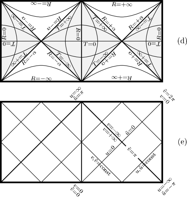
Figure 5: Coordinates in de Sitter space

(a) Regions I–IV are specified. They correspond to the same regions as in the cut $\mathcal{C}$ in Fig. 3. Coordinate lines of the conformally Einstein coordinates (b), of the conformally flat coordinates (c), of the static coordinates (d), and of the null coordinates (e), are indicated. For the definition of all these coordinate systems, see Eqs. (A.90)–(A.100). All the figures describe the same cut of de Sitter space. The ranges of coordinates covering the cut, as well as directions in which they grow, can be seen from the figures.

Commonly used are static coordinates $T$, $R$, related to the time-like Killing vector ${\frac{\partial}{\partial T}}$ of de Sitter spacetime:

$$\begin{aligned} T&=\frac{\alpha}{2}\,\log\frac{t^{2}-r^{2}}{\alpha^{2}}=\frac{\alpha}{2}\,\log\frac{\cos{\tilde{r}}-\cos{\tilde{t}}}{\cos{\tilde{r}}+\cos{\tilde{t}}}{\mbox{\;,\quad}}&T&\in{\mathbb{R}}{\mbox{\;,}}\\ R&=\alpha\;\frac{r}{t}=\alpha\,\frac{\sin{\tilde{r}}}{\sin{\tilde{t}}}{\mbox{\;,\quad}}&R&\in\langle 0,\alpha\rangle{\mbox{\;,}}\end{aligned}$$ (A.94)

$$g=-\Bigl{(}1-\frac{R^{2}}{\alpha^{2}}\Bigr{)}\mathrm{d}T{}^{\,2}+\Bigl{(}1-\frac{R^{2}}{\alpha^{2}}\Bigr{)}^{\!\!-1}\mathrm{d}R{}^{\,2}+R^{2}{\mathrm{d}\omega^{2}}{\mbox{\;.}}$$ (A.95)

As it is well-known, these coordinates do not cover the whole spacetime but only the domain with ${\tilde{t}}+{\tilde{r}}<\pi$ and ${\tilde{t}}-{\tilde{r}}>0$. The boundary of this domain is the Killing horizon. The coordinate $R$ can be extended smoothly to the whole spacetime but it is not unique globally. It is also useful to rescale coordinate $R$ to obtain the expanded static coordinates ${\bar{t}}$, ${\bar{r}}$:

$$\begin{aligned} {\bar{t}}&=T{\mbox{\;,\quad}}&{\bar{t}}&\in{\mathbb{R}}{\mbox{\;,}}\\ {\bar{r}}&=\alpha\;\operatorname{arctanh}\frac{R}{\alpha}{\mbox{\;,\quad}}&{\bar{r}}&\in{\mathbb{R}}{\mbox{\;,}}\end{aligned}$$ (A.96)

$$g=\Bigl{(}\cosh\frac{{\bar{r}}}{\alpha}\Bigr{)}^{-2}\;\Bigl{(}-\mathrm{d}{\bar{t}}{}^{\,2}+\mathrm{d}{\bar{r}}{}^{\,2}+\alpha^{2}\sinh^{2}\!\frac{{\bar{r}}}{\alpha}\;\,{\mathrm{d}\omega^{2}}\Bigr{)}{\mbox{\;.}}$$ (A.97)

Coordinate lines for the static coordinates are drawn in Fig. 5(d).

Finally, three sets of null coordinates $\{u,v\}$, $\{{\bar{u}},{\bar{v}}\}$, and $\{{\tilde{u}},{\tilde{v}}\}$ are defined by

$$u =t-r{\mbox{\;,\quad}} {\tilde{u}} ={\tilde{t}}-{\tilde{r}}{\mbox{\;,\quad}} {\bar{u}} ={\bar{t}}-{\bar{r}}{\mbox{\;,}}$$ (A.98)

$$v =t+r{\mbox{\;,\quad}} {\tilde{v}} ={\tilde{t}}+{\tilde{r}}{\mbox{\;,\quad}} {\bar{v}} ={\bar{t}}+{\bar{r}}{\mbox{\;.}}$$

From here we find

$$u=\alpha\,\tan\frac{{\tilde{u}}}{2}=\alpha\,\exp{\frac{{\bar{u}}}{\alpha}}{\mbox{\;,\quad}}v=\alpha\,\tan\frac{{\tilde{v}}}{2}=\alpha\,\exp{\frac{{\bar{v}}}{\alpha}}{\mbox{\;.}}$$ (A.99)

The metric in these coordinates reads

$$g =\frac{\alpha^{2}}{(u+v)^{2}}\;\Bigl{(}-2\,\mathrm{d}u\vee\mathrm{d}v+(u-v)^{2}\,{\mathrm{d}\omega^{2}}\Bigr{)}$$ (A.100)

$$=\frac{\alpha^{2}}{1-\cos({\tilde{v}}+{\tilde{u}})}\;\Bigl{(}-\,\mathrm{d}{\tilde{v}}\vee\mathrm{d}{\tilde{u}}+\bigl{(}1-\cos({\tilde{v}}-{\tilde{u}})\bigr{)}\,{\mathrm{d}\omega^{2}}\Bigr{)}$$

$$=\bigl{(}e^{{\bar{u}}/\alpha}+e^{{\bar{v}}/\alpha}\bigr{)}^{\!-2}\;\Bigl{(}-2\,e^{({\bar{u}}+{\bar{v}})/\alpha}\;\mathrm{d}{\bar{u}}\vee\mathrm{d}{\bar{v}}+\alpha^{2}\,\bigl{(}e^{{\bar{u}}/\alpha}-e^{{\bar{v}}/\alpha}\bigr{)}^{2}\,{\mathrm{d}\omega^{2}}\Bigr{)}{\mbox{\;.}}$$

The corresponding coordinate lines are illustrated in Fig. 5(e).

References

- [1] Modern Cosmology in Retrospect, edited by B. Bertotti, R. Balbinot, S. Bergia, and A. Messina (Cambridge University, Cambridge, England, 1990).
- [2] P. J. E. Peebles, Principles of Physical Cosmology (Princeton University, Princeton, 1993).
- [3] K. Maeda, Cosmic No-Hair Conjecture, in Proceedings of the Fifth M. Grossman Meeting on General Relativity, Perth, Australia, 1988, edited by D. G. Blair, M. J. Buckingham, and R. Ruffini (World Scientific, Singapore, 1989).
- [4] N. D. Birrell and P. C. W. Davies, Quantum Fields in Curved Space (Cambridge University, Cambridge, 1982).
- [5] B. de Witt and I. Herger, Anti-de Sitter Supersymetry, in Towards Quantum Gravity, Lecture Notes in Physics Vol. 541, (Springer-Verlag, New York, 2000), p. 79.
- [6] S. W. Hawking and G. F. R. Ellis, The Large Scale Structure of Space-time (Cambridge University, Cambridge, 1973).
- [7] R. Penrose, Asymptotic properties of fields and space-times, Phys. Rev. Lett. 10, 66 (1963).
- [8] R. Penrose, Zero rest-mass fields including gravitation: asymptotic behaviour, Proc. R. Soc. London A284, 159 (1965).
- [9] R. Penrose, Conformal treatment of infinity, in Relativity, Groups and Topology, Les Houches 1963, edited by C. DeWitt and B. DeWitt (Gordon and Breach, New York, 1964).
- [10] R. Penrose and W. Rindler, Spinors and Space-time (Cambridge University, Cambridge, 1984).
- [11] R. Penrose, Cosmological boundary conditions for zero rest-mass fields, in The nature of time, edited by T. Gold (Cornell University, Ithaca, NY, 1967), pp. 42–54.
- [12] Internal Structure of Black Holes and Spacetime Singularities, edited by L. Burko and A. Ori (Institute of Physics, and The Israel Physical Society, Bristol, Jerusalem, 1997).
- [13] E. Eriksen and Ø. Grøn, Electrodynamics of Hyperbolically Accelerated Charges I, II, III, Ann. Phys. (N.Y.) 286, 320 (2000).
- [14] J. Bičák, Selected Solutions of Einstein’s Field Equations: Their Role in General Relativity and Astrophysics, in Einstein’s Field Equations and Their Physical Implications, edited by B. G. Schmidt, Lecture Notes in Physics Vol. 540, (Springer, Berlin, 2000), pp. 1–126, e-print: gr-qc/0004016.
- [15] J. Bičák and B. G. Schmidt, Asymptotically flat radiative space-times with boost-rotation symmetry: the general structure, Phys. Rev. D 40, 1827 (1989).
- [16] J. Plebański and M. Demiański, Rotating charged and uniformly accelerated mass in general relativity, Ann. Phys. (N.Y.) 98, 98 (1976).
- [17] R. B. Mann and S. F. Ross, Cosmological production of charged black holes pairs, Phys. Rev. D 52, 2254 (1995).
- [18] J. Podolský and J. B. Griffiths, Uniformly accelerating black holes in a de Sitter universe, Phys. Rev. D 63, 024006 (2001).
- [19] C. W. Misner, K. S. Thorne, and J. A. Wheeler, Gravitation (Freeman, San Francisco, 1973).
- [20] R. M. Wald, General Relativity (The University of Chicago, Chicago, 1984).
- [21] T. Fulton, F. Rohrlich, and L. Witten, Conformal Invariance in Physics, Rev. Mod. Phys. 34, 442 (1962).
- [22] F. Rohrlich, Classical Charged Particles (Addison-Wesley, Reading, MA, 1965).
- [23] H. J. Vega, J. Ramirez, and N. Sanchez, Generation of gravitational waves by generic sources in de Sitter space-time, Phys. Rev. D 60, 044007 (1999).
- [24] J. Bičák and P. Krtouš, (unpublished).
- [25] H. J. Schmidt, On the de Sitter space-time — the geometric foundation of inflationary cosmology., Fortschr. Phys. 41, 179 (1993).
- [26] E. Eriksen and Ø. Grøn, The de Sitter universe models, Int. J. Mod. Phys. D 4, 115 (1995).