Evolution systems for non-linear perturbations of background geometries

Abstract

The formulation of the initial value problem for the Einstein equations is at the heart of obtaining interesting new solutions using numerical relativity and still very much under theoretical and applied scrutiny. We develop a specialised background geometry approach, for systems where there is non-trivial a priori knowledge about the spacetime under study. The background three-geometry and associated connection are used to express the ADM evolution equations in terms of physical non-linear deviations from that background. Expressing the equations in first order form leads naturally to a system closely linked to the Einstein-Christoffel system, introduced by Anderson and York, and sharing its hyperbolicity properties. We illustrate the drastic alteration of the source structure of the equations, and discuss why this is likely to be numerically advantageous.

I Introduction

An ongoing research effort, numerical relativity, attempts to solve the partial differential equations (PDEs) pertaining to the Einstein equations using numerical methods. A significant current focus is centered on the study of the relativistic two-body problem [1]. The broad features of the dynamics are already approximately known, through well established semi-analytical approaches, including perturbation theory (see e.g., a review in [2]) and post-Newtonian approximations (see e.g., latest developments in [3] and references therein). It seems intuitively right that one should be able to leverage such knowledge and reduce the computational complexity of the problem. There have been recently a number of proposals on various non-standard physical approximations to the spacetimes involved in mergers [4, 5, 6, 7]. A common theme among such proposals is the elimination of degrees of freedom which are thought of as not crucial for some phase of the computation. There is also presently activity on the mathematical notions underlying numerical relativity, with particular emphasis on the hyperbolicity properties of the equations (see e.g., [8]) and the nature of the propagation of the constraints. Even while the mathematical structure of the general problem is under scrutiny, there are particular instances of initial value problems which provide significant insights. For example, characteristic evolution of spacetimes that admit caustic-free foliations appear to be completely tractable [9]. Significant improvements have also been claimed using approaches which decompose the field variables in certain ways [10, 11].

We would like to advance in this paper a different perspective for numerical relativity. We will avoid any physical approximation to the equations, but we will try instead to pin down geometrically and analytically the system by introducing additional “guiding” structures in the spacetime manifold. The key concept will be a background geometry, constructed analytically, or semi-analytically, and encompassing the a priori knowledge about the system. The true dynamics will then unfold as a “correction” on the background. The proposal is promising on several grounds. It is easy to show that reformulating the evolution in terms of finite perturbations can lead to significant gains in accuracy for systems that never deviate significantly from the background. This is also borne out in preliminary computations. It is possible that the stability of computations will improve as well. This is much harder to ascertain concretely. We note that currently the main avenues for improving stability are sought in the direction of securing hyperbolicity properties and the convergence of the constraints, but this effort has not been conclusive. The relevance of source terms seems less well understood.

The concept of a background geometry has already been used in analytic studies of initial value problems (see e.g., in [12]), and it has also been claimed that the use of a background spacetime clarifies the task of defining energy and momentum quantities for the gravitational field [13]. The treatment presented in [12] is particularly enlightening for the motivation of this paper. There, two four-dimensional metrics are introduced on the spacetime manifold $M$. One of them, say $g_{\mu\nu}$, is promoted to physical status by virtue of satisfying the Einstein equations. The other, $\bar{g}_{\mu\nu}$, is relegated to a background role. Its associated Christoffel symbols, $\bar{\Gamma}^{\mu}{}_{\nu\rho}$, are used for the construction of a covariant derivative $\bar{\nabla}_{\mu}$. It is this derivative with respect to which one then expresses all relevant differential equations, e.g., gauge conditions and the Einstein equations. The fundamental evolution variables are the inverse metric differences $\chi^{\mu\nu}=g(g^{\mu\nu}-\bar{g}^{\mu\nu})\,,$ where $g$ is the determinant of the $g^{\mu\nu}$ metric. With the imposition of the harmonic gauge, $\bar{\nabla}_{\mu}\chi^{\mu\nu}=0\,,$ one obtains the reduced set of Einstein’s equations,

$\displaystyle g^{\rho\sigma}\bar{\nabla}_{\rho}\bar{\nabla}_{\sigma}\chi^{\mu\nu}+\mbox{L.O.T.}^{\mu\nu}=-2\bar{R}^{\mu\nu}+\bar{g}^{\mu\nu}\bar{R}\,,$where $\mbox{L.O.T.}^{\mu\nu}$ denotes terms of order lower than two and barred quantities in the right-hand side are the Ricci curvatures and scalars associated with the four dimensional background metric. Two remarks are worthwhile here. First, if $\bar{g}_{\mu\nu}$ is any exact solution of $\bar{R}^{\mu\nu}=0$ then the RHS of this equation is zero, which reflects the importance of the background for the structure of the source terms. Second, the hyperbolic characteristic structure of the equation is transparent, given its resemblance to a system of wave equations. It is noteworthy that whereas the source structure is background dependent, the hyperbolic structure solely relies on the physical metric.

Following this example, we will formulate here the Einstein evolution problem with a view towards numerical applications. To this end we will work within the framework of the 3+1 decomposition. There are several reasons for opting for this path in view of the above mentioned (covariant) examples. Maybe most importantly, we would like to have explicit control over the gauge functions, as we would like to construct them using a priori information. Additionally, the 3+1 decomposition is tightly linked to a Hamiltonian framework. We will not explicitly exploit this feature here, but this will ultimately facilitate a systematic use of background spacetimes derived from post-Newtonian approximate solutions.

The main result of this paper is the introduction of a set of new 3+1 evolution systems for the Einstein equations which explicitly separate a background geometry. The sets of evolution variables denote the finite deviations of the physical geometry from the assumed background. We derive systems involving second or first order spatial derivatives, with a corresponding change in the number of variables. In both cases we write the equations in a form which can explicitly cancel stationary or quasi-stationary balance terms, provided that adequate a priori description of those terms exists. We found that implementing the background geometry concept in conjunction with a hyperbolic system requires a slightly generalised geometrical construction. We will hence talk about the strong and weak versions of the proposal, according to the strength of the assumptions on the specifications of the physical and background spacetimes. All systems are constructed as three-covariant with respect to the background metric.

The structure of the paper is as follows. In section II we review some results in order to establish the notation. In Section III we will describe a framework based on the introduction of a background spatial metric and develop the geometric objects emerging in this picture. We then write evolution equations for the spatial tensors describing the deviation of the physical geometry from a background one. The two natural sets emerging are closely related to the ADM and Einstein-Christoffel systems. We argue that the metric compatibility condition in the latter is more properly seen as a geometric identity on the three dimensional Riemann tensor. In Section IV we will generalise the framework slightly, in order to develop a symmetric hyperbolic system for appropriate evolution fields. In Section V we make a number of remarks. We discuss implementation issues and a number of potential applications.

II Preliminaries and Notation

We will adopt the signature conventions used in [14]. Throughout the paper, Greek indices denote spacetime indices running from 0 to 3, whereas Latin indices are spatial indices and run from 1 to 3. Parentheses and square brackets will denote symmetrization and antisymmetrization respectively. Reference to geometric objects like vectors and tensors will refer to spatial objects, unless otherwise stated. We will systematically use an overbar to distinguish geometrical objects referring to a background geometry. Raising and lowering of indices will always be using the physical metric. We will consider only the vacuum case, i.e., absence of matter sources ($T_{\mu\nu}=0$). Studies of matter systems (in particular fluids) along similar lines are pursued separately [15] and a generalisation will be given elsewhere.

The 3+1 decomposition (also known as the Arnowitt-Deser-Misner (ADM) formulation) of Einstein’s equations [16] has been discussed in detail in many works (see, e.g., [17]). It assumes that the spacetime has topology $R\times\Sigma$, and hence it is foliated by the level surfaces $\Sigma(t)$ of a scalar function $t(x^{\mu})$. The unit normal to the hypersurfaces $\Sigma(t)$, $n^{\mu}=-N\nabla^{\mu}t$, satisfies $g_{\mu\nu}n^{\mu}n^{\nu}+1=0$. It can be used to decompose the four-metric as

$$g_{\mu\nu}=h_{\mu\nu}-n_{\mu}n_{\nu}\,.$$ (1)

The vector field $t^{\mu}$ (time threading of the manifold, $t^{\mu}\nabla_{\mu}t=1$) giving rise to the relations $N=-t^{\mu}n_{\mu}$ and $\beta^{\mu}=t^{\mu}-Nn^{\mu}$ allows to write the metric element in the form

$$ds^{2}=-N^{2}dt^{2}+h_{ij}(dx^{i}+\beta^{i}dt)(dx^{j}+\beta^{j}dt)\,.$$ (2)

Here, $N$ is the lapse scalar, which is assumed to be positive, $\beta^{i}$ is the spatial shift vector, and $h_{ij}$ is the spatial metric (or first fundamental form) induced on the hypersurfaces $\Sigma(t)$.

In terms of the unit normal, the second fundamental form or extrinsic curvature of the spatial hypersurfaces is given by

$$K_{ij}=-\textstyle{1\over 2}{\pounds}_{n}h_{ij}~{}~{}\Rightarrow~{}~{}\hat{\partial}_{t}h_{ij}=-2NK_{ij}\,,$$ (3)

where the time operator is $\hat{\partial}_{t}=\partial_{t}-{\pounds}_{\beta}$, and ${\pounds}_{\beta}$ denotes Lie differentiation with respect to $\beta^{i}$. In particular,

$${\pounds}_{\beta}h_{ij}=\beta^{k}\partial_{k}h_{ij}+h_{ik}\partial_{j}\beta^{k}+h_{jk}\partial_{i}\beta^{k}=2D_{(i}\beta_{j)}\,,$$ (4)

where $\beta_{i}=h_{ij}\beta^{j}$. The Einstein equations are decomposed in a set of evolution equations for the components of the extrinsic curvature

$$\hat{\partial}_{t}K_{ij}=-D_{i}D_{j}N+N(R_{ij}+KK_{ij}-2K_{i}{}^{l}K_{jl})\,,$$ (5)

the momentum constraint

$$D_{j}K^{j}{}_{i}-D_{i}K=0\,,$$ (6)

and the Hamiltonian constraint

$$R+K^{2}-K^{ij}K_{ij}=0\,.$$ (7)

In these equations $K=h^{ij}K_{ij}$, $D_{i}$, $R_{ij}$, and $R$ are the canonical covariant derivative, Ricci tensor, and scalar curvature associated with the spatial metric $h_{ij}$ respectively. The Einstein field equations are equivalent to the evolution equations (3) and (5) together with the constraints (6) and (7). Given initial data on an initial hypersurface $\Sigma(t_{o})$, i.e. $(h^{o}_{ij},K^{o}_{ij})$ satisfying the constraints, and freely specifiable quantities $N$ and $\beta^{i}$ defined for all $\Sigma(t)$, one can use the evolution equations to find the future development of such data. The framework is explicitly three-covariant.

III 3+1 decomposition with background metric: Strong version

We assume a second spatial metric field, denoted by $\bar{h}_{ij}$, cohabiting with $h_{ij}$ on each of the hypersurfaces $\Sigma(t)$. The four-dimensional manifold $M$ is then endowed with an additional four-metric defined by

$$\bar{g}^{\mu\nu}=\bar{h}^{\mu\nu}-n^{\mu}n^{\nu}\,,$$ (8)

where

$$\bar{h}^{\mu\nu}n_{\nu}=0\hskip 11.38109pt\mbox{and}\hskip 11.38109pt\bar{h}^{ij}=(\mbox{\boldmath$\bar{h}^{-1}$})^{ij}\,.$$ (9)

The normal $n^{\mu}=g^{\mu\nu}n_{\nu}$ is now a unit normal vector with respect to both metrics. Then, there is a unique projection operator onto the hypersurfaces $\Sigma(t)$, $h^{\mu}{}_{\nu}=\bar{h}^{\mu}{}_{\nu}=\delta^{\mu}{}_{\nu}+n^{\mu}n_{\nu}$. As is clear, this construction uses the same lapse $N$ and shift vector $\beta^{i}$ for both spacetimes and hence the name strong version. Taking into account the relations $N=-t^{\mu}n_{\mu}$ and $\beta^{\mu}=t^{\mu}-Nn^{\mu}$ we write the background metric in the form

$$ds^{2}=-N^{2}dt^{2}+\bar{h}_{ij}(dx^{i}+\beta^{i}dt)(dx^{j}+\beta^{j}dt)\,.$$ (10)

The extrinsic curvature associated with the background geometry can be computed from the expression

$$\bar{K}_{\mu\nu}=-\bar{h}_{(\mu}{}^{\rho}\bar{h}_{\nu)}{}^{\sigma}\bar{\nabla}_{\sigma}n_{\rho}\,,$$ (11)

where $\bar{\nabla}_{\mu}$ is the connection associated with the background spacetime metric $\bar{g}_{\mu\nu}$. This leads to

$$\bar{K}_{ij}=-\textstyle{1\over 2}{\pounds}_{n}\bar{h}_{ij}~{}~{}\Rightarrow~{}~{}\hat{\partial}_{t}\bar{h}_{ij}=-2N\bar{K}_{ij}\,.$$ (12)

The two spatial metrics give rise to compatible covariant derivatives $D_{i}$ and $\bar{D}_{i}$ satisfying $D_{i}h_{jk}=0$ and $\bar{D}_{i}\bar{h}_{jk}=0$. If $\bar{\Gamma}^{i}{}_{jk}$ denotes the Christoffel symbols associated with $\bar{h}_{ij}$ then ${\cal E}^{i}{}_{jk}=\Gamma^{i}{}_{jk}-\bar{\Gamma}^{i}{}_{jk}$, the difference of the Christoffel symbols, is also a tensor. Indeed, under a coordinate change $x^{i}\rightarrow x^{i^{\prime}}=f^{i^{\prime}}(x^{i})$, the Christoffel symbols transform as

$\displaystyle\Gamma^{i^{\prime}}{}_{j^{\prime}k^{\prime}}=\frac{\partial x^{i^{\prime}}}{\partial x^{i}}\Gamma^{i}{}_{jk}\frac{\partial x^{j}}{\partial x^{j^{\prime}}}\frac{\partial x^{k}}{\partial x^{k^{\prime}}}+\frac{\partial x^{i^{\prime}}}{\partial x^{l}}\frac{\partial^{2}x^{l}}{\partial x^{j^{\prime}}\partial x^{k^{\prime}}}\,,$whence the tensorial transformation law for ${\cal E}^{i}{}_{jk}$ follows

$\displaystyle{\cal E}^{i^{\prime}}{}_{j^{\prime}k^{\prime}}=\frac{\partial x^{i^{\prime}}}{\partial x^{i}}{\cal E}^{i}{}_{jk}\frac{\partial x^{j}}{\partial x^{j^{\prime}}}\frac{\partial x^{k}}{\partial x^{k^{\prime}}}\,.$In fact, the explicitly covariant expression for ${\cal E}^{i}{}_{jk}$ is

$${\cal E}^{i}{}_{jk}=\textstyle{1\over 2}h^{il}(\Delta_{jkl}+\Delta_{kjl}-\Delta_{ljk})\,,$$ (13)

where

$$\Delta_{kij}=\bar{D}_{k}h_{ij}\,.$$ (14)

We see that $\Delta_{kij}$ is the covariant derivative of the physical spatial metric with respect to the background spatial canonical connection. The two covariant derivatives acting on a general tensor field are related by

$$D_{i}{\cal A}^{j\cdots}{}_{k\cdots}=\bar{D}_{i}{\cal A}^{j\cdots}{}_{k\cdots}+{\cal E}^{j}{}_{il}{\cal A}^{l\cdots}{}_{k\cdots}+\cdots-{\cal E}^{l}{}_{ik}{\cal A}^{j\cdots}{}_{l\cdots}-\cdots\,.$$ (15)

Pictorially our geometric construct is presented in Fig. 1. The unit normal vector field $n^{\mu}$ represents Eulerian observers momentarily at rest on the hypersurface $\Sigma(t)$ and is by construction the same for both spacetimes. The acceleration 1-form of those observers, $a_{\mu}=n^{\nu}\nabla_{\nu}n_{\mu}$, (with $a^{\mu}n_{\mu}=0$), is the same as seen from both spacetimes. Some calculations show that

$$\bar{a}_{\mu}=\bar{h}_{\mu}{}^{\nu}\bar{\nabla}_{\nu}(\ln N)=h_{\mu}{}^{\nu}\nabla_{\nu}(\ln N)=a_{\mu}\,,$$ (16)

where we have used the fact that the background and physical four-covariant derivative have the same action on the scalar $\ln N$.

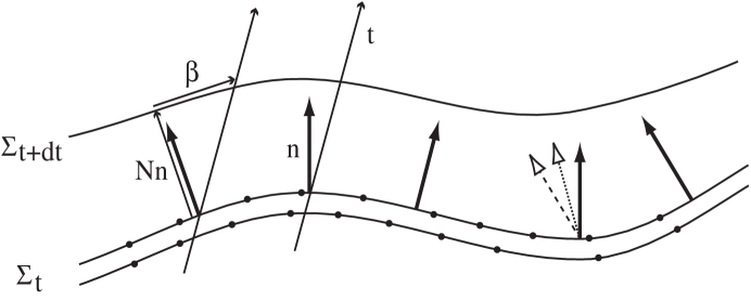
FIG. 1.: 3+1 decomposition and a background geometry. Two dimensions are suppressed for practical reasons. Two successive level surfaces of the time scalar are shown, with corresponding unit normal vectors in bold arrows. The standard decomposition of the time flow vector field into the lapse and shift components are shown. All those elements are independent of the intrinsic 3-metric. The two different intrinsic geometries are also shown, as two different copies of hypersurface $\Sigma(t)$ (which should be thought as overlapping). The filled circles on the hypersurface can be thought of as markers of equal proper length, thus indicating the different intrinsic curvature. The effects on the extrinsic curvature are also indicated. The right-most normal vector, when parallel transported to the left using the physical metric produces the dashed vector. The difference of this vector from the local normal (bold vector) is the physical extrinsic curvature. The same original normal parallel transported under the background metric, gives rise to the dotted vector, implying a different (background) extrinsic curvature.

A Time evolution equations and constraints

We turn now to the task of writing the 3+1 decomposed Einstein equations in terms of a background metric. One further identity we will need relates the Ricci tensors of the two metrics (see, e.g., [12]) in terms of ${\cal E}^{i}_{jk}$. Using the explicitly symmetric form of the Ricci tensor, such an identity is:

$$R_{ij}-\bar{R}_{ij}=\bar{D}_{k}{\cal E}^{k}{}_{ij}-\bar{D}_{(i}{\cal E}^{k}{}_{j)k}+{\cal E}^{k}{}_{ij}{\cal E}^{l}{}_{kl}-{\cal E}^{k}{}_{l(i}{\cal E}^{l}{}_{j)k}\,.$$ (17)

We rewrite the basic evolution system in the following form:

$$\hat{\partial}_{t}h_{ij} = -2NK_{ij}\,,$$ (18)

$$\hat{\partial}_{t}K_{ij} = -\bar{D}_{i}\bar{D}_{j}N+\bar{D}_{k}(N{\cal E}^{k}{}_{ij})-N\bar{D}_{(i}{\cal E}^{k}{}_{j)k}$$ (20)

$$+N{\cal E}^{k}{}_{ij}{\cal E}^{l}{}_{kl}-N{\cal E}^{k}{}_{l(i}{\cal E}^{l}{}_{j)k}+N(KK_{ij}-2K_{i}{}^{l}K_{jl})+N\bar{R}_{ij}\,,$$

where we have used the relation (15) to convert covariant derivatives with respect to the connection $\bar{D}_{i}$ into covariant derivatives with respect to $\bar{D}_{i}$. Moreover, the Lie derivatives in the time operator $\hat{\partial}_{t}$ are expanded as

$${\pounds}_{\beta}h_{ij}=\beta^{k}\bar{D}_{k}h_{ij}+h_{ik}\bar{D}_{j}\beta^{k}+h_{jk}\bar{D}_{i}\beta^{k}\,,$$ (21)

and

$${\pounds}_{\beta}K_{ij}=\beta^{k}\bar{D}_{k}K_{ij}+K_{ik}\bar{D}_{j}\beta^{k}+K_{jk}\bar{D}_{i}\beta^{k}\,.$$ (22)

In the above equations, ${\cal E}^{i}_{jk}$ is shorthand for equations (13,14). Hence this is the classic ADM form of the evolution system, but expressed using a background metric and connection.

It will be useful here to introduce an alternative expression for Eq. (20). This form of the equation (for Gaussian coordinates) is given in [18] and to write it we introduce a densitized extrinsic curvature (of weight $1$)

$${\cal K}^{i}{}_{j}=h^{\frac{1}{2}}h^{ik}K_{kj}\,,$$ (23)

where $h$ is the determinant of the three-metric $h_{ij}$. The evolution of this quantity can be found through the definition of the extrinsic curvature (which implies the evolution equations $\hat{\partial}_{t}h=-2hNK$ and $\hat{\partial}_{t}h^{ij}=2NK^{ij}$)

$$h^{-\frac{1}{2}}h_{il}\hat{\partial}_{t}{\cal K}^{l}{}_{j}=-NKK_{ij}+2NK_{i}{}^{l}K_{jl}+\hat{\partial}_{t}K_{ij}\,.$$ (24)

Combining this expression with the evolution of $K_{ij}$ [Eq. (20)] we get

$$\hat{\partial}_{t}{\cal K}^{i}{}_{j} = h^{\frac{1}{2}}h^{ik}\left\{-\bar{D}_{k}\bar{D}_{j}N+\bar{D}_{l}(N{\cal E}^{l}{}_{kj})-N\bar{D}_{(k}{\cal E}^{l}{}_{j)l}+N{\cal E}^{l}{}_{kj}{\cal E}^{m}{}_{lm}\right.-N{\cal E}^{l}{}_{m(k}{\cal E}^{m}{}_{j)l}\left.+N\bar{R}_{kj}\right\}\,,$$ (25)

Equation (25) departs from the standard form of ADM evolution systems, which explicitly preserve the symmetry of the extrinsic curvature and hence only require six components. Instead here one obtains the evolution to nine components, which satisfy the three additional constraints

$$h_{l[i}{\cal K}^{l}{}_{j]}=0\,.$$ (26)

A direct symmetrization, ${\cal K}^{{}^{\prime}}_{ij}=h_{l(i}{\cal K}^{l}{}_{j)}$, e.g., after each evolution step in a numerical algorithm, would be sufficient for enforcing those constraints.

An evolution equation for ${\cal E}^{i}_{jk}$ can be computed in the following way: first, using the evolution equation for $h_{ij}$ [Eq. (3)] and the Ricci identities for the commutation of spatial derivatives

$$(D_{i}D_{j}-D_{j}D_{i}){\cal A}^{k\cdots}{}_{l\cdots}=R^{k}{}_{mij}{\cal A}^{m\cdots}{}_{l\cdots}+\cdots-R^{m}{}_{lij}{\cal A}^{k\cdots}{}_{m\cdots}-\cdots\,,$$ (27)

where $R^{i}{}_{jkl}$ denotes the Riemann tensor of $h_{ij}$, one can find that

$$\partial_{t}\Gamma^{i}{}_{jk}=D_{(j}D_{k)}\beta^{i}-R^{i}{}_{(jk)l}\beta^{l}+D^{i}(NK_{jk})-2D_{(j}(NK_{k)}{}^{i})\,.$$ (28)

On the other hand, the Lie derivative of the Christoffel symbols is a tensor that can be expressed as follows [28]

$${\pounds}_{\beta}\Gamma^{i}{}_{jk}=D_{j}D_{k}\beta^{i}-R^{i}{}_{kjl}\beta^{l}\,.$$ (29)

Combining Eqs. (28) and (29) we get

$$\hat{\partial}_{t}\Gamma^{i}{}_{jk}=D^{i}(NK_{jk})-2D_{(j}(NK_{k)}{}^{i})\,.$$ (30)

which re-expressed for the background geometry reads

$$\hat{\partial}_{t}{\cal E}^{i}{}_{jk}=h^{il}\left\{\bar{D}_{l}(NK_{jk})-2\bar{D}_{(j}(NK_{k)l})+2N{\cal E}^{m}{}_{jk}K_{ml}\right\}+\hat{\partial}_{t}\bar{\Gamma}^{i}{}_{jk}\,,$$ (31)

where $\hat{\partial}_{t}\bar{\Gamma}^{i}{}_{jk}$ has to be replaced by the corresponding background version of Eq. (30).

With the promotion of the components of the tensor ${\cal E}^{i}{}_{jk}$ to independent variables, we must re-examine the additional constraints those variables must satisfy. The first one concerns the metric compatibility of the connection, i.e., $D_{i}h_{jk}=0$ which, expressed in terms of the background connection, is equivalent to the definition of ${\cal E}^{i}{}_{jk}$ [Eq. (13)], or to the following relationship

$$\bar{D}_{k}h_{ij}=2{\cal E}_{(ij)k}\,,\hskip 14.22636pt\mbox{where}\hskip 8.53581pt{\cal E}_{ijk}=h_{il}{\cal E}^{l}{}_{jk}\,.$$ (32)

Another condition, which can be seen as a consequence of (32), is the metric-induced property of the Riemann tensor of $h_{ij}$

$$R_{ijkl}+R_{jikl}=0\,.$$ (33)

In our framework, this condition expresses the fact that the action of the commutator of background covariant derivatives, $[\bar{D}_{i},\bar{D}_{j}]$, when applied to the physical metric, is given by the usual rule

$\displaystyle(\bar{D}_{k}\bar{D}_{l}-\bar{D}_{l}\bar{D}_{k})h_{ij}=-2h_{m(i}\bar{R}^{m}{}_{j)kl}\,.$This in particular contains the relation $\bar{D}_{[i}{\cal E}^{k}{}_{j]k}=0$ which has been used to write the differences between Ricci tensors (17) in an explicitly symmetric form.

B Non-linear perturbations

In the previous subsection we introduced a number of systems which made explicit use of the existence of a background spatial metric. The spatial connection tensor ${\cal E}^{k}{}_{ij}$ arose naturally with the consideration of a background metric. In contrast, we will need to explicitly introduce “perturbative” spatial metric and extrinsic curvature tensors. To simplify the notation we will use the symbol $\delta$ to denote “perturbative” quantities: $\mbox{\boldmath$\delta$}{\cal A}^{i\ldots}{}_{j\ldots}={\cal A}^{i\ldots}{}_{j\ldots}-\bar{{\cal A}}^{i\ldots}{}_{j\ldots}$. Then, the relation between the “perturbative” spatial metric and extrinsic curvature tensors

$\displaystyle\phi_{ij}=\mbox{\boldmath$\delta$}h_{ij}=h_{ij}-\bar{h}_{ij}\,,\hskip 11.38109pt\psi_{ij}=\mbox{\boldmath$\delta$}K_{ij}=K_{ij}-\bar{K}_{ij}\,,$is given by

$$\hat{\partial}_{t}\phi_{ij}=-2N\psi_{ij}\,.$$ (34)

On the other hand, we can always write the following evolution equation for the background extrinsic curvature

$$\hat{\partial}_{t}\bar{K}_{ij}=-\bar{D}_{i}\bar{D}_{j}N+N(\bar{R}_{ij}+\bar{K}\bar{K}_{ij}-2\bar{K}_{i}{}^{l}\bar{K}_{jl})-\bar{S}_{ij}\,,$$ (35)

which has to be considered as the definition of $\bar{S}_{ij}$. In the special case where ($\bar{h},\bar{K},N,\beta$) is an exact solution of the Einstein equations, Eq. (35) reduces to $\bar{S}_{ij}=0$ and can be interpreted as the dynamical evolution of an alternative initial data set $(\bar{h}^{o}_{ij},\bar{K}^{o}_{ij})$.

Subtracting Eq. (35) from Eq. (20) eliminates terms involving second derivatives of the lapse and the background Ricci curvature and introduces additional extrinsic curvature terms,

$$\hat{\partial}_{t}\psi_{ij}=\bar{D}_{k}(N{\cal E}^{k}{}_{ij})-N\bar{D}_{(i}{\cal E}^{k}{}_{j)k}+N{\cal E}^{k}{}_{ij}{\cal E}^{l}{}_{kl}-N{\cal E}^{k}{}_{l(i}{\cal E}^{l}{}_{j)k}+N\mbox{\boldmath$\delta$}(KK_{ij}-2K_{i}{}^{l}K_{jl})+\bar{S}_{ij}\,.$$ (36)

The extrinsic curvature terms can be absorbed with the use of the densitized variable ${\cal K}^{i}{}_{j}$ [see Eq. (23)] for both the physical and background spacetimes. Then, we can write the following alternative equation for the evolution of the components of the extrinsic curvature

$$\hat{\partial}_{t}\mbox{\boldmath$\delta$}{\cal K}^{i}{}_{j}=h^{\frac{1}{2}}h^{ik}\left\{\bar{D}_{l}(N{\cal E}^{l}{}_{jk})-N(\bar{D}_{(j}{\cal E}^{l}{}_{k)l}-{\cal E}^{l}{}_{jk}{\cal E}^{m}{}_{lm}+{\cal E}^{l}{}_{m(j}{\cal E}^{m}{}_{k)l})+\eta_{kl}\hat{\partial}_{t}\bar{{\cal K}}^{l}{}_{j}+\bar{S}_{jk}\right\}\,,$$ (37)

where

$$\eta_{ij}=-\mbox{\boldmath$\delta$}(h^{-\frac{1}{2}}h_{ij})=(\bar{h}^{-\frac{1}{2}}-h^{-\frac{1}{2}})\bar{h}_{ij}-h^{-\frac{1}{2}}\phi_{ij}\,.$$ (38)

It is worth noting that in equation (37) background Ricci terms have been eliminated. The choice of an exact background solution would eliminate $\bar{S}_{ij}$ as well. The term involving $\hat{\partial}_{t}\bar{{\cal K}}^{m}{}_{j}$ will be different from zero in general, but it is homogeneous in the metric deviations from the background.

The expression of the evolution equation for ${\cal E}^{i}{}_{jk}$ [Eq. (31)] in terms of the “perturbative” and background quantities is the following

$$\hat{\partial}_{t}{\cal E}^{i}{}_{jk} = N\left\{h^{il}(\bar{D}_{l}\psi_{jk}-2\bar{D}_{(j}\psi_{k)l})+\mbox{\boldmath$\delta$}h^{il}(\bar{D}_{l}\bar{K}_{jk}-2\bar{D}_{(j}\bar{K}_{k)l})\right.$$ (40)

$$\left.+2h^{il}{\cal E}^{m}{}_{jk}(\psi_{lm}+\bar{K}_{lm})\right\}+[h^{il}\psi_{jk}+\phi^{il}\bar{K}_{jk}-2\psi_{(j}{}^{i}\delta_{k)}{}^{l}]\bar{D}_{l}N\,,$$

where $\psi_{j}{}^{i}=\mbox{\boldmath$\delta$}K_{j}{}^{i}$ and $h^{ij}$ must be understood in terms of $\phi_{ij}$ and $\bar{h}_{ij}$, i.e. $h^{ij}=([\mbox{\boldmath$\phi$}+\mbox{\boldmath$\bar{h}$}]^{-1})^{ij}$.

In summary, utilising the background geometry and identifying the key geometric variables we have derived four evolution systems, for the sets of fields $(h_{ij},K_{ij})$, $(h_{ij},{\cal K}_{ij})$, $(\phi_{ij},\psi_{ij},{\cal E}^{i}{}_{jk})$ and $(\phi_{ij},\mbox{\boldmath$\delta$}{\cal K}_{ij},{\cal E}^{i}{}_{jk})$ respectively. All those equations are formulated in terms of the background metric and connection, but the physical metric also appears explicitly. In addition, background source terms, e.g., $\bar{R}_{ij}$, $\hat{\partial}_{t}\bar{\Gamma}^{i}{}_{jk}$ are present.

IV 3+1 decomposition with background metric: Weak version and hyperbolicity

In what follows we introduce a modified version of the framework described in Sec. III. As before, in addition to the physical metric $h_{ij}$ we assume a second metric field, denoted by $\bar{h}_{ij}$, cohabiting with $h_{ij}$ on each of the hypersurfaces $\Sigma(t)$, but instead of considering the same unit normal vector we consider a new one $\bar{n}^{\mu}$ which we assume to be parallel to the physical one $n^{\mu}$, i.e. $\bar{n}^{\mu}=\lambda n^{\mu}$ ($\lambda>0$). We can combine these objects to define a background four-metric in the following way

$$\bar{g}^{\mu\nu}=\bar{h}^{\mu\nu}-\bar{n}^{\mu}\bar{n}^{\nu}=\bar{h}^{\mu\nu}-\lambda^{2}n^{\mu}n^{\nu}\,,$$ (41)

where $\bar{h}^{\mu\nu}$ satisfies the same conditions as in the strong version [see Eq. (9)]. The condition that $\bar{n}^{\mu}$ is a unit normal vector with respect to $\bar{g}_{\mu\nu}=\bar{h}_{\mu\nu}-\lambda^{-2}n_{\mu}n_{\nu}$ ($\bar{h}_{\mu\nu}\bar{n}^{\nu}=0$) reflects the fact that the lapse scalar for the background is different from that of the physical spacetime. We will call it $\bar{N}$ and assume is a strictly positive function. Then, we can take $\lambda=N/\bar{N}$ and therefore the relation between normals can be written as

$$\bar{n}^{\mu}=\frac{N}{\bar{N}}n^{\mu}\hskip 11.38109pt\mbox{and}\hskip 11.38109pt\bar{n}_{\mu}=\frac{\bar{N}}{N}n_{\mu}\,.$$ (42)

With the assumptions made in this weak version of the 3+1 framework there is still a unique projection operator onto the hypersurfaces $\Sigma(t)$, $h^{\mu}{}_{\nu}=\bar{h}^{\mu}{}_{\nu}=\delta^{\mu}{}_{\nu}+n^{\mu}n_{\nu}=\delta^{\mu}{}_{\nu}+\bar{n}^{\mu}\bar{n}_{\nu}$.

Using the relations $\bar{N}=-t^{\mu}\bar{n}_{\mu}$ and $\beta^{\mu}=t^{\mu}-\bar{N}\bar{n}^{\mu}=t^{\mu}-Nn^{\mu}$ we write the background line-element as

$$ds^{2}=-\bar{N}^{2}dt^{2}+\bar{h}_{ij}(dx^{i}+\beta^{i}dt)(dx^{j}+\beta^{j}dt)\,.$$ (43)

Pictorially, the current geometric construction is presented in Fig. 2. The Eulerian observers associated with the background metric follow the same worldlines as the corresponding observers in the physical spacetime, but their acceleration is different: $\bar{a}_{i}=\bar{D}_{i}(\ln\bar{N})$ as opposed to $a_{i}=D_{i}(\ln N)$. Therefore, some of the rigidity in the correspondence between physical and background spacetimes is lost, but one still has a unique time evolution operator, $\hat{\partial}_{t}$, which is a consequence of having the same shift spatial vector $\beta^{i}$ in both constructions.

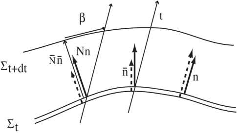
FIG. 2.: 3+1 decomposition on a background geometry: weak version. Two successive level surfaces of the time scalar are shown, with two sets of corresponding unit normal vectors (in bold and dashed arrows). The decomposition of the time flow vector field into the lapse and shift components is shown for the two possible lapse alternatives. The essence of the construction is that in order to advance from the level hypersurface $\Sigma(t)$ to $\Sigma(t+dt)$ one uses the same time operator $\hat{\partial}_{t}=\partial_{t}-{\pounds}_{\beta}$.

As in Sec. III, the second fundamental form associated with the background geometry can be constructed from the expression (11), which leads to the usual relation between spatial metric and extrinsic curvature

$$\bar{K}_{ij}=-\textstyle{1\over 2}{\pounds}_{\bar{n}}\bar{h}_{ij}~{}~{}\Rightarrow~{}~{}\hat{\partial}_{t}\bar{h}_{ij}=-2\bar{N}\bar{K}_{ij}\,.$$ (44)

A First order systems and hyperbolicity

The evolution equations for $(h_{ij},K_{ij},{\cal E}^{i}{}_{jk})$, (18), (20) and (31), as they stand do not satisfy any hyperbolicity condition, which implies that we cannot formulate a well-posed initial-value problem (see [8, 20]). There are many ways of reformulating Einstein’s equations in order to get a hyperbolic system of partial differential equations (see [8, 23, 25] and references therein). The structure of the equations for $(h_{ij},K_{ij},{\cal E}^{i}{}_{jk})$ suggests that the hyperbolicity properties will be very closely linked to the first-order symmetric hyperbolic formulation introduced recently in [22]. This has been named the “Einstein-Christoffel” (EC) system, which is based in considering combinations of the variables $(h_{ij},K_{ij},\Gamma^{i}{}_{jk})$. In [26], implementing this formulation by means of a pseudospectral collocation scheme, a stable evolution of spherically symmetric black holes with horizon excision has been achieved, and in [27], the total evolution time of 3D black hole computations has been extended by using EC type systems.

As in the EC formulation [22], instead of considering the lapse $N$ as a freely specifiable scalar function, we will arbitrarily prescribe the scalar density (of weight $-1$) $\alpha$, which in the case of the physical metric is defined through the following expression

$$N(\alpha,h)=\alpha h^{\frac{1}{2}}\,,~{}~{}\mbox{where}~{}~{}h=\mbox{det}(h_{ij})\,.$$ (45)

This automatically changes the principal part of the evolution equation for the extrinsic curvature [Eq. (5)], which will be crucial for the hyperbolic structure of the final evolution equations (see [23] for details). This way of prescribing the gauge precludes the possibility of choosing the background lapse $\bar{N}$ to be the same as the one of the physical spacetime $N$, which is the main motivation for the weak formulation of the 3+1 framework given above. Instead, one can introduce a background densitized lapse $\bar{\alpha}$ as above

$$\bar{N}(\bar{\alpha},\bar{h})=\bar{\alpha}\bar{h}^{\frac{1}{2}}\,.$$ (46)

We start the construction of the hyperbolic formulation with the evolution equation for the spatial metric “perturbation” $\phi_{ij}$, which reads as

$$\hat{\partial}_{t}\phi_{ij}=-2N\psi_{ij}-2\mbox{\boldmath$\delta$}N\,\bar{K}_{ij}\,,\hskip 11.38109pt\mbox{where}\hskip 11.38109pt\mbox{\boldmath$\delta$}N=N-\bar{N}\,,$$ (47)

and where $N$ and $\bar{N}$ must be understood as given by the expressions (45) and (46) respectively. Notice that now we have a source term proportional to the difference of lapses which did not appear in the previous formulation.

With regard to the evolution equation for the extrinsic curvature “perturbation” $\psi_{ij}$, we must first rewrite the term $\bar{D}_{i}\bar{D}_{j}N$ in term of $\alpha$. Taking into account the expression for the covariant derivative of a scalar density $\sigma$ of weight $w$, $D_{i}\sigma=\partial_{i}\sigma-w\Gamma^{j}{}_{ij}\sigma$, it becomes

$\displaystyle\bar{D}_{i}\bar{D}_{j}N=\bar{D}_{(i}(N{\cal E}^{k}{}_{j)k})+h^{\frac{1}{2}}\left\{\bar{D}_{i}\bar{D}_{j}\alpha+{\cal E}^{k}{}_{k(i}\bar{D}_{j)}\alpha\right\}\,.$As is clear, this modifies the principal part of the equation for $K_{ij}$ (20). The result can be written as follows

$$\hat{\partial}_{t}K_{ij} = \bar{D}_{k}(N{\cal E}^{k}{}_{ij})-2\bar{D}_{(i}(N{\cal E}^{k}{}_{j)k})+N({\cal E}^{k}{}_{ij}{\cal E}^{l}{}_{kl}+2{\cal E}^{[k}{}_{k(i}{\cal E}^{l]}{}_{j)l}+KK_{ij}$$ (49)

$$-2K_{i}{}^{l}K_{jl}+\bar{R}_{ij})-h^{\frac{1}{2}}\bar{D}_{i}\bar{D}_{j}\alpha\,.$$

Then, the equation for $\psi_{ij}$ takes the form

$$\hat{\partial}_{t}\psi_{ij} = \bar{D}_{k}(N{\cal E}^{k}{}_{ij})-2\bar{D}_{(i}(N{\cal E}^{k}{}_{j)k})+N({\cal E}^{k}{}_{ij}{\cal E}^{l}{}_{kl}+2{\cal E}^{[k}{}_{k(i}{\cal E}^{l]}{}_{j)l})$$ (51)

$$+\mbox{\boldmath$\delta$}\left[N(KK_{ij}-2K_{i}{}^{l}K_{jl})\right]+\mbox{\boldmath$\delta$}N\,\bar{R}_{ij}+\bar{h}^{\frac{1}{2}}\bar{D}_{i}\bar{D}_{j}\bar{\alpha}-h^{\frac{1}{2}}\bar{D}_{i}\bar{D}_{j}\alpha\,.$$

Finally, the equation for ${\cal E}^{i}{}_{jk}$ is

$$\hat{\partial}_{t}{\cal E}^{i}{}_{jk} = h^{il}\left\{\bar{D}_{l}(NK_{jk})-2\bar{D}_{(j}(NK_{k)l})+2NK_{lm}{\cal E}^{m}{}_{jk}\right\}$$ (53)

$$+\bar{h}^{il}\left\{2\bar{D}_{(j}(\bar{N}\bar{K}_{k)l})-\bar{D}_{l}(\bar{N}\bar{K}_{jk})\right\}\,.$$

The system of partial differential equations we have got for $(\phi_{ij},\psi_{ij},{\cal E}^{i}{}_{jk})$ [Eqs. (47), (51), and (53)] is still not explicitly symmetric hyperbolic. We can get such form by introducing a new quantity, with the same number of independent components as ${\cal E}^{i}{}_{jk}$ (eighteen), which will be considered as a fundamental variable [22]

$$\zeta_{kij}=\textstyle{1\over 2}\Delta_{kij}-h_{k(i}h^{lm}(\Delta_{|lm|j)}-\Delta_{j)lm})={\cal E}_{(ij)k}+h_{k(i}h^{lm}({\cal E}_{|lm|j)}-{\cal E}_{j)lm})\,.$$ (54)

The inverse relations are

$$\Delta_{kij} = 2\left\{\zeta_{kij}+2h_{k(i}h^{lm}[\zeta_{j)lm}-\zeta_{|lm|j)}]\right\}\,,$$ (55)

$${\cal E}_{ijk} = 2\zeta_{(jk)i}-\zeta_{ijk}+4h_{jk}h^{lm}\zeta_{[il]m}\,.$$ (56)

Then, let us look for a system of evolution equations for the unknowns $(\phi_{ij},\psi_{ij},\zeta_{ijk})$. As is clear, Eq. (47) remains the evolution equation for $\phi_{ij}$. The evolution equation for $\psi_{ij}$ is obtained by replacing ${\cal E}^{i}{}_{jk}$ by $\zeta_{ijk}$ in Eq. (49). The procedure to carry out this calculation is to express first ${\cal E}^{i}{}_{jk}$ in terms of $\Delta_{ijk}$ [Eq. (14)] and then to use the following important property of $\Delta_{ijk}$

$$\bar{D}_{[l}\Delta_{k]ij}=-h_{m(i}\bar{R}^{m}{}_{j)lk}\,,$$ (57)

which follows from the Ricci identities (27). The quantity analogous to $\Delta_{ijk}$ in the EC formulation is ${\cal G}_{kij}=\partial_{k}h_{ij}$. It satisfies the analogous simpler relation $\partial_{[k}{\cal G}_{l]ij}=0$. These relations constitute one of the keys to find a explicitly symmetric hyperbolic system. Once the property (57) has been used, we have to express $\Delta_{ijk}$ in terms of $\zeta_{ijk}$ [Eq. (55)]. After some calculations we obtain

$$\hat{\partial}_{t}\psi_{ij} = -N\left\{h^{kl}\bar{D}_{k}\zeta_{lij}-{\cal E}^{k}{}_{ij}{\cal E}^{l}{}_{kl}+2{\cal E}^{(k}{}_{k(i}{\cal E}^{l)}{}_{j)l}+\textstyle{1\over 2}(\bar{R}_{ij}+h^{kl}\bar{R}^{m}{}_{kl(i}h_{j)m})\right.$$ (61)

$$-2h^{kl}h^{mn}\left[\zeta_{ikm}\zeta_{jln}+2(\zeta_{kl(i}-\zeta_{(i|kl|})(\zeta_{j)mn}-\zeta_{|mn|j)})-2\zeta_{(i|km|}(\zeta_{j)ln}-\zeta_{|ln|j)})\right.$$

$$\left.\left.+2\zeta_{kij}(\zeta_{lmn}-\zeta_{mnl})\right]\right\}+\mbox{\boldmath$\delta$}\left[N(KK_{ij}-2K_{i}{}^{l}K_{jl})\right]+\mbox{\boldmath$\delta$}N\,\bar{R}_{ij}$$

$$+h^{\frac{1}{2}}({\cal E}^{k}{}_{ij}\bar{D}_{k}\alpha-2{\cal E}^{k}{}_{k(i}\bar{D}_{j)}\alpha-\bar{D}_{i}\bar{D}_{j}\alpha)+\bar{h}^{\frac{1}{2}}\bar{D}_{i}\bar{D}_{j}\bar{\alpha}\,,$$

where ${\cal E}^{i}{}_{jk}$ must be understood as given by expression (56).

To find the evolution equation for $\zeta_{kij}$ we have to apply $\hat{\partial}_{t}$ to the expression (54) and use all the information we have. It turns out that in order to have the desired form for the principal of this equation one needs to make use of the momentum constraint (6) that the physical spacetime has to satisfy. After some manipulations the result is

$$\hat{\partial}_{t}\zeta_{kij} = -\bar{D}_{k}(NK_{ij})+4NK_{k(i}h^{lm}[\zeta_{j)lm}-\zeta_{|lm|j)}]+2Nh_{k(i}[K_{j)}{}^{l}h^{mn}-\delta_{j)}{}^{l}K^{mn}]{\cal E}_{lmn}$$ (64)

$$+4h^{\frac{1}{2}}h_{k(i}\delta_{j)}{}^{m}h^{ln}K_{l[m}[\bar{D}_{n]}\alpha+\alpha{\cal E}^{p}{}_{n]p}]+h_{k(i}\bar{D}_{j)}(\bar{N}\bar{K})+h_{l(i}[\bar{D}_{j)}(\bar{N}\bar{K}_{k}{}^{l})$$

$$+\bar{D}_{|k|}(\bar{N}\bar{K}_{j)}{}^{l})-\bar{D}^{l}(\bar{N}\bar{K}_{j)k})]-h_{k(i}h_{j)n}h^{lm}[2\bar{D}_{l}(\bar{N}\bar{K}_{m}{}^{n})-\bar{D}^{n}(\bar{N}\bar{K}_{lm})]\,.$$

At this point we have a system of first-order evolution equations for the unknowns $(\phi_{ij},\psi_{ij},\zeta_{kij})$ [Eqs. (47), (61) and (64)], where some quantities constructed from $(h_{ij},K_{ij})$ appear explicitly but they must be considered as given by their expressions in terms of $(\phi_{ij},\psi_{ij})$ and $(\bar{h}_{ij},\bar{K}_{ij})$. We finish this section by showing the differential structure of the system (47,61,64). This analysis is standard (see, e.g., [8]) and one only needs to consider the principal part of the equations, which for our system looks as follows

$$\hat{\partial}_{t}\phi_{ij} \approx 0\,,$$ (65)

$$\hat{\partial}_{t}\psi_{ij} \approx -Nh^{kl}\bar{D}_{k}\zeta_{lij}\,,$$ (66)

$$\hat{\partial}_{t}\zeta_{kij} \approx -N\bar{D}_{k}\psi_{ij}\,,$$ (67)

where $\approx$ means equality up to terms that do not contain derivatives of the unknowns $(\phi_{ij},\psi_{ij},\zeta_{kij})$. From the structure of the principal part we deduce that the system is symmetric hyperbolic. Indeed, the equations that determine the kernel of the principal symbol associated with the system are

$$(\mbox{\boldmath$n$}\cdot\mbox{\boldmath$\xi$})\phi_{ij}=0\,,$$ (68)

$$(\mbox{\boldmath$n$}\cdot\mbox{\boldmath$\xi$})\psi_{ij}+\xi^{k}\zeta_{kij}=0\,,$$ (69)

$$(\mbox{\boldmath$n$}\cdot\mbox{\boldmath$\xi$})\zeta_{kij}+\xi_{k}\psi_{ij}=0\,,$$ (70)

where $\mbox{\boldmath$\xi$}=(\xi_{t},\xi_{i})$ is an arbitrary covector, $\mbox{\boldmath$n$}\cdot\mbox{\boldmath$\xi$}=g^{\mu\nu}n_{\mu}\xi_{\nu}=n^{\mu}\xi_{\mu}$, and $\xi^{i}=h^{ij}\xi_{j}$. From the structure of the principal symbol it follows that the characteristic directions of propagation of the system are the normal to the spacelike hypersurfaces, $\mbox{\boldmath$n$}\cdot\mbox{\boldmath$\xi$}=0$, and the light cone determined by the physical metric $(\mbox{\boldmath$n$}\cdot\mbox{\boldmath$\xi$})^{2}=1$, and therefore, as in the EC formulation, the characteristic speeds are the speed of light and the zero speed. From the analysis of the kernel of the principal symbol we deduce that the fields propagating along the normal to the hypersurfaces $\Sigma(t)$ are all the components of $\phi_{ij}$ and 12 components of $\zeta_{kij}$, namely

$\displaystyle\zeta_{kij}=A_{k}\xi_{i}\xi_{j}+2B_{k(i}\xi_{j)}+C_{kij}\,,$where $A_{i}$, $B_{ij}$, and $C_{kij}$ satisfy: $\xi^{i}A_{i}=\xi^{i}B_{ij}=\xi^{i}C_{kij}=0$. The fields propagating along the physical null cone are all the components of $\psi_{ij}$ and the 6 components of $\zeta_{kij}$ given by

$$\psi_{ij} = D\xi_{i}\xi_{j}+2E_{(i}\xi_{j)}+F_{ij}\,,$$ (71)

$$\zeta_{kij} = \epsilon(D\xi_{k}\xi_{i}\xi_{j}+\xi_{k}F_{ij}+2\xi_{k}\xi_{(i}E_{j)})\,,$$ (72)

where now $\epsilon=\mbox{\boldmath$n$}\cdot\mbox{\boldmath$\xi$}$ ($\epsilon=\pm 1$) and the quantities $E_{i}$ and $F_{ij}$ are such that $\xi^{i}E_{i}=\xi^{i}F_{ij}=0$.

Finally, as it is usual in the theory of symmetric hyperbolic PDEs, we can introduce an energy norm for our system [Eqs. (47), (61) and (64)] which is given by

$\displaystyle\mbox{E}(t)=\int_{\Sigma(t)}(\phi^{ij}\phi_{ij}+\psi^{ij}\psi_{ij}+\zeta^{kij}\zeta_{kij})\,\mbox{\boldmath$d\Sigma$}\,,$where $d\Sigma$ is the volume element of $\Sigma(t)$ and indices are raised using the inverse spatial physical metric $h^{ij}$.

V Summary and discussion

The main results of this paper are the introduction of a set of new evolution systems for the Einstein equations which explicitly separate a background geometry. We have studied two broad classes, which differ slightly in their geometrical construction. An important realisation has been that for constructing a hyperbolic set of evolution equations one must relax the assumption of a common lapse. The reason lies with the fact that the use of a densitized lapse is important for inducing the appropriate modification to the principal part of the equations. This introduces a gauge function that incorporates information about the three metric. On the other hand, having a background spacetime which shares the same lapse and shift as the physical one is crucial for a maximal simplification of the resulting equations. The choices are summarised in Fig. 3. The introduction of a background geometry makes all the systems explicitly three-covariant. Besides a certain aesthetic appeal, this feature may be handy in applications involving multiple coordinate systems, e.g., spherical coordinate patches adapted to black holes and infinity respectively.

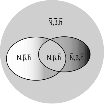
FIG. 3.: The logical relationship between different possible arrangements for the background geometry. In the most general case (enclosing set), the background geometry has both its gauge functions (lapse and shift) different from the physical geometry. The use of a common lapse or shift vector defines the two inner sets. For the overlap of those two sets, both lapse and shift are the same as for the physical spacetime. This arrangement corresponds to the framework in Section II (strong version). The developments in Section III (weak version) refer to the set on the right, characterised by $(\bar{N},\beta,\bar{h})$.

We note that in determining the light-cone structure, or in the case of the first order systems, the propagation of eigenfields, it is the physical metric that is always the governing field. This implies that there would be no unpleasant side-effects associated with the choice of a background spacetime that is causally incompatible with the physical one. We have not elaborated on the Hamiltonian and momentum constraints. Those are essential for the construction of consistent initial data. The conformal techniques and decompositions involved in reducing those equations to well behaved elliptic systems seem at first glance not to be particularly benefiting from the assumption of a generic background geometry.

A key issue that must be considered is the way in which the use of a background geometry would modify the numerical properties of evolution equations for the Einstein system. Common to most approaches to the evolution problem is the solution of a quasi-linear system of explicitly or implicitly hyperbolic equations with sources. For spacetimes involving compact objects, large curvature gradients are present. Those gradients survive in the stationary (non-dynamical limit) and involve a balance between flux terms in the principal part of the equation and the source terms. The source terms are not homogeneous in the evolution fields which can also be expressed as the existence of longitudinal modes. For fluid spacetimes (e.g., neutron stars) this balance has physical underpinnings in the fluid pressure supporting the star. For black holes it is geometric in nature.

The implementation of the systems developed here can proceed in a number of manners. After a suitable choice of background geometry, a direct discretization of the equations using standard discrete approximations is possible. A practise usually adopted is to ignore the constraint equations in the construction of the algorithm (free evolution) and to monitor them as time dependent error norms. The integration of a physical data set will then consist of a sequence of discrete timesteps into the future. In principle, for a stable and convergent algorithm, the solution can be found at any future finite time to any desired accuracy given enough resolution. With the use of prescribed background geometry one has the flexibility of a more interactive approach to the time evolution, namely through an iteration of the evolution process. This technique could be useful in circumstances in which the background geometry is constructed analytically on the basis of a few poorly known parameters, e.g., post-Newtonian locations and momenta of black holes. The iterations would then provide improved estimates for those parameters. Whereas any of the iterative steps can in principle converge to the true solution, it has been our argument that the residual errors will be dramatically reduced as one improves the guess on the background spacetime.

The incorporation of matter dynamics has not been discussed here. There is no specific obstruction to the process. In contrary, an implementation of closely related non-linear perturbation concepts to the relativistic Euler equations is already underway with promising results [15]. An optimal application candidate would be the study of non-linear perturbations of a single black hole spacetime. In this case the stationary exact black hole solutions provide readily available first guesses for the background geometry. More speculative, but well motivated, is the application to multiple black hole systems. Here the appropriate construction of an approximate spacetime would make heavy use of post-Newtonian solutions. The framework provides a well defined path for systematically incorporating post-Newtonian results into the full PDE evolution, which only hinges on the suitable expansion of post-Newtonian results into global metric data.

Acknowledgements: We warmly thank M. Bruni, P. Laguna, and R. Maartens for comments on the manuscript. CFS acknowledges support from the European Commission (contract HPMF-CT-1999-00149). PP acknowledges support from the EU Programme “Improving the Human Research and Socio-Economic Knowledge Base” (Research training network HPRN-CT-2000-00137) and the Nuffield Foundation (award NAL/00405/G).

REFERENCES

- [1] G. B. Cook et al. (The Binary Black Hole Grand Challenge Alliance), Phys. Rev. Lett. 80, 2512 (1998).
- [2] J. Pullin, Prog. Theor. Phys. Suppl. 136, 107 (1999).
- [3] T. Damour (gr-qc/0103018).
- [4] G. J. Mathews, P. Marronetti, and J. R. Wilson, Phys. Rev. D 58, 043003 (1998).
- [5] P. R. Brady, J. D. E. Creighton, and K. S. Thorne, Phys. Rev. D 58, 061501 (1998).
- [6] P. Laguna, Phys. Rev. D 60, 084012 (1999).
- [7] J. Baker, M. Campanelli, and C. Lousto (gr-qc/0104063).
- [8] H. Friedrich, Class. Quantum Grav. 13, 1451 (1996).
- [9] R. Gomez et al. (The Binary Black Hole Grand Challenge Alliance), Phys. Rev. Lett. 80, 3915 (1998).
- [10] M. Shibata and T. Nakamura, Phys. Rev. D 52, 5428 (1995).
- [11] T. W. Baumgarte and S. L. Shapiro, Phys. Rev. D 59, 024007 (1999).
- [12] S. W. Hawking and G. F. R. Ellis, The large scale structure of space-time (Cambridge University Press, Cambridge, 1973).
- [13] L. P. Grishchuk, A. N. Petrov, and A. D. Popova, Commun. Math. Phys. 94, 379 (1984).
- [14] C. W. Misner, K. S. Thorne, and J. A. Wheeler, Gravitation (Freeman and Co., New York, 1973).
- [15] U. Sperhake, P. Papadopoulos, and N. Andersson, submitted (2001).
- [16] R. Arnowitt, S. Deser and C. W. Misner, in Gravitation: An introduction to current research, edited by L. Witten (Wiley, New York, 1962) 227.
- [17] J. W. York, in Sources of gravitational radiation, edited by L. L. Smarr (Cambridge University Press, Cambridge, 1979) 83; R. M. Wald, General Relativity (The University of Chicago Press, Chicago, 1984).
- [18] L. D. Landau and E. M. Lifshitz, The Classical Theory of Fields (Translation from Russian original: Pergamon Press, Oxford, 1975).
- [19] S. Frittelli and O. A. Reula, Phys. Rev. Lett. 76, 4667 (1996).
- [20] O. A. Reula, Hyperbolic Methods for Einstein’s Equations (Living Reviews, article 1998-3).
- [21] A. D. Rendall, Local and global existence theorems for the Einstein equations (Living Reviews, article 1998-4).
- [22] A. Anderson and J. W. York, Phys. Rev. Lett. 82, 4384 (1999).
- [23] A. Anderson, Y. Choquet-Bruhat and J. W. York, in Proceedings of the 2nd Samos Meeting on Cosmology, Geometry and Relativity: Mathematical and Quantum aspects of Relativity and Cosmology, edited by S. Cotsakis and G. W. Gibbons (Lecture notes in Physics, Springer, Berlin, 2000) 30.
- [24] S. Frittelli and O. A. Reula, J. Math. Phys. 40, 5143 (1999).
- [25] H. Friedrich and A. D. Rendall, The Cauchy problem for the Einstein equations (gr-qc/0002074).
- [26] L. E. Kidder, M. A. Scheel, S. A. Teukolsky, E. D. Carlson and G. B. Cook, Phys. Rev. D 62, 084032 (2000).
- [27] L. E. Kidder, M. A. Scheel, and S. A. Teukolsky, Phys. Rev. D 64, 064017 (2001).
- [28] J. A. Schouten, Ricci calculus (Springer, Berlin, 1954).