Gravitational signals emitted by a point mass orbiting a neutron star: a perturbative approach

Abstract

We compute the energy spectra of the gravitational signals emitted when a pointlike mass moves on a closed orbit around a non rotating neutron star, inducing a perturbation of its gravitational field and its internal structure. The Einstein equations and the hydrodynamical equations are perturbed and numerically integrated in the frequency domain. The results are compared with the energy spectra computed by the quadrupole formalism which assumes that both masses are pointlike, and accounts only for the radiation emitted because the orbital motion produces a time dependent quadrupole moment. The results of our perturbative approach show that, in general, the quadrupole formalism overestimates the amount of emitted radiation, especially when the two masses are close. However, if the pointlike mass is allowed to move on an orbit so tight that the keplerian orbital frequency resonates with the frequency of the fundamental quasi-normal mode of the star ($2\omega_{K}=\omega_{f}$), this mode can be excited and the emitted radiation can be considerably larger than that computed by the quadrupole approach.

I Introduction

The coalescence of binary systems composed of compact objects like black holes or neutron stars is considered one of the most promising sources of gravitational waves to be detected by ground-based interferometers. For this reason it is important to collect as much information as possible on the features of the gravitational signal emitted in these processes. This paper focuses on the phenomena which may occur during the pre-merging phase of the coalescence, when the two stars are still individual bodies in fast revolution around each other. The problem of computing the energy spectrum and the waveforms of the gravitational waves emitted in this regime can be attacked by using different approaches. The easiest is the quadrupole formalism, which assumes that the two stars are pointlike masses, and computes the emitted radiation in terms of the quadrupole moment of the system, whose time variation is due to the orbital motion. When the two stars get very close, post newtonian corrections can be included to give a more accurate description of the trajectories, and to refine the orbital contribution of the emitted radiation. These calculations can be complemented by the inclusion of radiation reaction effects, which account for the shrinking of the orbit caused by the emission of gravitational waves.

This approach clearly overlooks the fact that the two stars are extended bodies with an internal structure and that, when they are close, the tidal interaction becomes strong and new effects, unpredictable by the quadrupole + post-newtonian approaches, may arise. An accurate description of these phases of the coalescence requires the solution of the Einstein equations coupled with those of hydrodynamics in the non-linear regime, and many groups in the world are working in this direction [1]. These studies will certainly yield new and interesting results, but a complete picture is still far from reaching; indeed, due to the complexity of this phenomenon the computational tools presently available allow to follow the evolution of the system for no more than a few orbits near coalescence. Waiting for the results of fully non linear simulations, it is interesting to explore other techniques that, though approximated, allow to get some insight into those phases of the coalescence where the quadrupole + post-newtonian approaches are inadequate. For instance, we can assume that one of the two stars is a “true star”, i.e. it is an extended body whose equilibrium structure is described by a solution of the relativistic equations of hydrostatic equilibrium, and that only the second star is a pointlike mass; its effect is to induce a perturbation on the gravitational field and on the thermodynamical structure of the extended companion, which can be evaluated by solving the equations of stellar perturbations in general relativity. In this way we can account for the tidal effects of the close interaction on one of the two stars and for their consequences on the gravitational emission, and get a clue on the kind of phenomena that could arise near coalescence. This approach has already been used in a previous paper [2] where we computed the energy spectrum of the gravitational radiation emitted when a pointlike mass moves on an open orbit around a compact star. In this paper we shall extend our investigation to the case of closed orbits, either circular or eccentric, and compute the energy spectra and the waveforms of the emitted radiation.

The purpose of our study is to compare the quadrupole radiation emitted by the system because of its orbital motion to the signal computed in the relativistic, perturbative approach.

The orbital emission will be computed using a hybrid quadrupole approach, which assumes that the pointlike mass moves on a geodesic of the spacetime generated by the star, but radiates, according to the standard quadrupole formula, as if it were in flat spacetime.

To evaluate the relativistic emission, the equations of stellar perturbations we integrate in the interior of the star are those derived in ref. [3]; therefore we shall not describe them in detail, but only recall the relevant formulae. In [2], outside the star we integrated the Sasaki-Nakamura equation [6]; here we consider closed orbits, i.e. a source with a compact support, and it is more convenient to integrate the Bardeen-Press-Teukolsky (BPT) equation [7, 8] whose source term has a much simpler form.

Since in this paper we do not consider the effects of radiation reaction, we cannot describe the evolution of the orbit and of the waveform during the inspiralling; thus the energy spectra we show have to be considered as representative of a certain number of orbital periods over which the radiation reaction effects do not produce a significant change in the orbital parameters of the pointlike mass (adiabatic approximation). These effects will be considered in a forthcoming paper.

Stellar perturbations excited by an orbiting particle have also been considered by Kojima [9], who focused on the energy enhancement with respect to the standard newtonian quadrupole formula, due to the excitation of the fundamental mode by a particle in circular orbit. The excitation of the $w$-modes has been studied by Ruoff, Laguna and Pullin in a time domain approach [10].

The plan of the paper is the following. In $\S$ II we write the equations relevant to our problem, in $\S$ III we discuss the source term of the BPT equation, in $\S$ IV we outline the integration procedure, and discuss how to find the power emitted in gravitational waves and the waveforms. In $\S$ V we show how to compute the same quantities by the hybrid quadrupole approach. Numerical results are discussed in $\S$ VI and conclusions are drawn in $\S$ VII.

II The perturbed equations

In order to describe the non-axisymmetric perturbations of a non rotating star induced by an orbiting mass we choose, as in [2], the following gauge

$$ds^{2} = e^{2\nu(r)}dt^{2}-e^{2\mu_{2}(r)}dr^{2}-r^{2}d\theta^{2}-r^{2}\sin^{2}\theta d\phi^{2}$$ (1)

$$+ \sum_{lm}~{}~{}\int^{+\infty}_{-\infty}d\omega~{}e^{-i\omega t}\Biggl{\{}2e^{2\nu}N_{lm}Y_{lm}dt^{2}-2e^{2\mu_{2}}L_{lm}Y_{lm}dr^{2}-2r^{2}H_{33}d\theta^{2}-2r^{2}\sin^{2}\theta H_{11}d\phi^{2}\Biggr{.}$$ (2)

$$- \Biggl{.}4r^{2}H_{13}d\theta d\phi+2\sin\theta\frac{\partial Y_{lm}}{\partial\theta}\left[h^{0}_{lm}dtd\phi+h^{1}_{lm}drd\phi\right]-\frac{2}{\sin\theta}\frac{\partial Y_{lm}}{\partial\phi}\left[h^{0}_{lm}dtd\theta+h^{1}_{lm}drd\theta\right]\Biggr{\}}$$ (3)

where the perturbed metric functions $[N_{lm},L_{lm},V_{lm},T_{lm},h^{0}_{lm},h^{1}_{lm}]$ are functions of $(\omega,r)$,  $Y_{lm}(\theta,\phi)$  are the scalar spherical harmonics, and

$$H_{11} = \left[T_{lm}+V_{lm}\left(\frac{1}{\sin^{2}{\theta}}\frac{\partial^{2}}{\partial\phi^{2}}+\cot{\theta}\frac{\partial}{\partial\theta}\right)\right]\ Y_{lm}$$ (4)

$$H_{13} = V_{lm}\left[\frac{\partial^{2}}{\partial\phi\partial\theta}-\frac{\partial}{\partial\phi}\cot\theta\right]Y_{lm}$$ (5)

$$H_{33} = \left[T_{lm}+V_{lm}\frac{\partial^{2}}{\partial\theta^{2}}\right]\ Y_{lm}\ .$$ (6)

The functions  $\Bigl{[}N_{lm},L_{lm},V_{lm},T_{lm}\Bigr{]},$  are the radial part of the polar (even) metric components, and  $h^{0}_{lm}$  and  $h^{1}_{lm}$  are the axial (odd) part.

The unperturbed metric functions  $\nu(r)$  and  $\mu_{2}(r)$  can be found by solving the equations of hydrostatic equilibrium (cfr. [2], Eqs. (2.2)-(2.4)) for an assigned equation of state. As in [2], we shall consider as a model a polytropic compact star,  $p=K\epsilon^{n},$  with  $K=100~{}km^{2}$  and  $n=2.$  If the central density is chosen to be  $\epsilon_{c}=3\cdot 10^{15}~{}g/cm^{3},$  the radius and mass of the star are, respectively,  $R_{s}=8.86~{}km$  and  $M=1.266~{}M_{\odot},$  with a ratio  $R_{s}/M=4.7.$  Although this model is, to some extent, unrealistic, it is appropriate to understand the basic features of the problem we want to study.

Inside the star, it is convenient to replace the perturbed metric functions $V_{lm}$ and $T_{lm}$ by two new functions

$$X = nV$$

$$G = \nu_{,r}[\frac{n+1}{n}X-T]_{,r}+\frac{1}{r^{2}}(e^{2\mu_{2}}-1)[n(N+T)+N]+\frac{\nu_{,r}}{r}(N+L)-$$

$$- e^{2\mu_{2}}(\epsilon+p)N+\frac{1}{2}\omega^{2}e^{2(\mu_{2}-\nu)}[L-T+\frac{2n+1}{n}X]\>.$$

where  $n=(l-1)(l+2)/2.$  The polar metric functions  $\Bigl{[}N_{lm},L_{lm},X_{lm},G_{lm}\Bigr{]}$  can be found by solving a set of linear coupled equations (cfr. [3], Eqs. 72-75), from which the fluid perturbations have been eliminated

$$X_{,r,r}+\left(\frac{2}{r}+\nu_{,r}-\mu_{2,r}\right)X_{,r}+\frac{n}{r^{2}}e^{2\mu_{2}}(N+L)+\omega^{2}e^{2(\mu_{2}-\nu)}X=0,$$ (7)

$$(r^{2}G){,r}=n\nu_{,r}(N-L)+\frac{n}{r}(e^{2\mu_{2}}-1)(N+L)+r(\nu_{,r}-\mu_{2,r})X_{,r}+\omega^{2}e^{2(\mu_{2}-\nu)}rX\;,$$ (8)

$$-\nu_{,r}N_{,r}=-G+\nu_{,r}[X_{,r}+\nu_{,r}(N-L)]+\frac{1}{r^{2}}(e^{2\mu_{2}}-1)(N-rX_{,r}-r^{2}G)$$ (9)

$$-e^{2\mu_{2}}(\epsilon+p)N+\frac{1}{2}\omega^{2}e^{2(\mu_{2}-\nu)}\left\{N+L+\frac{r^{2}}{n}G+\frac{1}{n}[rX_{,r}+(2n+1)X]\right\},$$ (10)

$$-L_{,r}=(N+2X)_{,r}+\left(\frac{1}{r}-\nu_{,r}\right)(-N+3L+2X)+$$ (11)

$$+\left[\frac{2}{r}-(Q+1)\nu_{,r}\right]\left[N-L+\frac{r^{2}}{n}G+\frac{1}{n}(rX_{,r}+X)\right]\;,$$ (12)

where  $Q=\left(\frac{\partial p}{\partial\epsilon}\right)^{-1}_{s}.$

The equations for the axial perturbation can be combined into a single wave equation by introducing a function  $Z^{ax}_{lm}(\omega,r)$  related to the axial functions by the following equations

$$h^{0}_{lm}=-\frac{i}{\omega}\frac{d}{dr_{*}}\left(rZ^{ax}_{lm}\right),\qquad\qquad h^{1}_{lm}=-e^{-2\nu}\left(rZ^{ax}_{lm}\right),$$ (13)

where  $r_{*}=\int_{0}^{r}e^{-\nu+\mu_{2}}dr.$  The equation  $Z^{ax}_{lm}(\omega,r)$  satisfies is (cfr. [3], Eqs. 148-149)

$$\frac{d^{2}Z^{ax}_{lm}}{dr_{*}^{2}}+\Biggl{\{}\omega^{2}-\frac{e^{2\nu}}{r^{3}}\Biggl{[}l(l+1)r+r^{3}(\epsilon-p)-6m(r)\Biggr{]}\Biggr{\}}Z^{ax}_{lm}=0,$$ (14)

which, outside the star, automatically reduces to the Regge-Wheeler equation [5]. The polar and axial equations (7) and (14) are numerically integrated from $r=0$, where we impose a regularity condition, up to the surface of the star $r=R_{s}$. There we compute the amplitudes of the Zerilli function [4]

$$Z^{pol}_{lm}(\omega,R_{s})=\frac{R_{s}}{nR_{s}+3M}\Bigl{[}\frac{3M}{n}X_{lm}(\omega,R_{s})-R_{s}L_{lm}(\omega,R_{s})\Bigr{]},$$ (15)

and of the Regge-Wheeler function,  $Z^{ax}_{lm}(\omega,R_{s}),$  and their first derivatives, which will be used to continue the solution outside the star.

To describe the perturbations of the Schwarzschild spacetime prevailing outside the star we use the BPT equation [7, 8]

$$\left\{\Delta^{2}\frac{d}{dr}\left[\frac{1}{\Delta}\frac{d}{dr}\right]+\left[\frac{\left(r^{4}\omega^{2}+4i(r-M)r^{2}\omega\right)}{\Delta}-8i\omega r-2n\right]\right\}\Psi_{lm}(\omega,r)=-T_{lm}(\omega,r),$$ (16)

where  $\Delta=r^{2}-2Mr,$  and the BPT function,  $\Psi_{lm},$  is related to the perturbation of the Weyl scalar  $\delta\Psi_{4}$  by

$$\Psi_{lm}(\omega,r)=\frac{1}{2\pi}\int d\Omega~{}dt~{}e^{i\omega t}~{}_{-2}S^{\ast}_{lm}(\theta,\phi)\left[r^{4}~{}\delta\Psi_{4}(t,r,\theta,\phi)\right],$$ (17)

where  ${}_{-2}S_{lm}(\theta,\phi)$  is the spin-weighted spherical harmonic

$${}_{-2}S_{lm}(\theta,\phi)=\frac{1}{2\sqrt{n(n+1)}}\Biggl{[}\frac{\partial^{2}Y_{lm}}{\partial\theta^{2}}-\cot\theta\frac{\partial Y_{lm}}{\partial\theta}+\frac{m^{2}}{\sin^{2}\theta}Y_{lm}\Biggr{.}$$ (18)

$$\Biggl{.}+\frac{2m}{\sin\theta}\left(\frac{\partial Y_{lm}}{\partial\theta}-Y_{lm}\cot\theta\right)\Biggr{]}.$$ (19)

The advantage of using the BPT equation is that  $\delta\Psi_{4}$  is invariant under gauge transformations and infinitesimal tetrad rotations, and that the squares of its real and imaginary parts are proportional to the energy flux of the outgoing radiation at infinity in the two polarizations. In addition, the source term  $T_{lm}(\omega,r),$  which will be discussed in detail in the next section, has a much simpler form than the source of the Sasaki-Nakamura equation which we used to study the gravitational emission in the case of open orbits in [2].

At the surface of the star, where  $T_{lm}(\omega,r)=0,$  the relation between  $\Psi_{lm},$    $Z^{pol}_{lm}$  and  $Z^{ax}_{lm}$  is

$$\Psi_{lm} = \frac{r^{3}\sqrt{n\left(n+1\right)}}{4\omega}\left[V^{ax}Z^{ax}_{lm}+\left(W^{ax}+2i\omega\right)\Lambda_{+}Z^{ax}_{lm}\right]$$ (20)

$$- \frac{r^{3}\sqrt{n\left(n+1\right)}}{4}\left[V^{pol}Z^{pol}_{lm}+\left(W^{pol}+2i\omega\right)\Lambda_{+}Z^{pol}_{lm}\right],$$ (21)

where  $\Lambda_{+}={d\over dr_{*}}+i\omega={\Delta\over r^{2}}{d\over dr}+i\omega,$  and

$$V^{ax} = {2\Delta\over r^{5}}\left[(n+1)r-3M\right]$$

$$W^{ax} = {2\over r^{2}}(r-3M)$$

$$V^{pol} = {2\Delta\over r^{5}(nr+3M)^{2}}\left[n^{2}(n+1)r^{3}+3Mn^{2}r^{2}+9M^{2}nr+9M^{3}\right]$$

$$W^{pol} = 2{nr^{2}-3Mnr-3M^{2}\over r^{2}(nr+3M)}.$$

According to (20) we can write  $\Psi_{lm}$  as a sum of an axial and a polar part, i.e.

$$\Psi_{lm}=\Psi_{lm}^{~{}ax}+\Psi_{lm}^{~{}pol},$$ (22)

where

$${\Psi}^{~{}ax}_{lm} = \frac{r^{3}\sqrt{n\left(n+1\right)}}{4\omega}\left[V^{ax}{Z}^{ax}_{lm}+\left(W^{ax}+2i\omega\right)\Lambda_{+}{Z}^{ax}_{lm}\right]$$ (23)

$${\Psi}^{~{}pol}_{lm} = -\frac{r^{3}\sqrt{n\left(n+1\right)}}{4}\left[V^{pol}{Z}^{pol}_{lm}+\left(W^{pol}+2i\omega\right)\Lambda_{+}{Z}^{pol}_{lm}\right].$$ (24)

However, in Section 4 we will show that depending on the value of the harmonic indices $l$ and $m$, only the polar or the axial part of  $\Psi_{lm}$  have to be selected.

III The source term of the BPT equation

We shall assume that the pointlike mass $m_{0}$ which excites the perturbations of the star follows a geodesic of the unperturbed spacetime on the equatorial plane, with energy  $E$  and angular momentum $L_{z}$, so that the geodesic equations are

$$\frac{dt}{d\tau}=\frac{E}{1-\frac{2M}{r}},~{}~{}~{}~{}\frac{dr}{d\tau}\equiv\gamma=\pm\sqrt{E^{2}-\left(1-\frac{2M}{r}\right)\left(1+\frac{L_{z}^{2}}{r^{2}}\right)},~{}~{}~{}~{}\frac{d\varphi}{d\tau}=\frac{L_{z}}{r^{2}}.$$ (25)

For a closed orbit the motion takes place between a periastron $r_{P}$ and an apoastron $r_{A}$, roots of the equation $\gamma=0$ (a third root marks the onset of a plunging motion, that is not relevant for our study). We can define the semi-latus rectum $p$ and the eccentricity $e$ in terms of $r_{P}$ and $r_{A}$ through the relations:

$$r_{P}=\frac{pM}{1+e},~{}~{}~{}~{}r_{A}=\frac{pM}{1-e}.$$ (26)

Both $p$ and $e$ are dimensionless, and they are, respectively, a measure of the size and of the degree of noncircularity of the orbit. Note that $0\leq e<1$. The orbit is periodic in the radial coordinate, and quasi-periodic in the $\varphi$-coordinate, i.e.

$$r(t+\Delta t)=r(t)$$ (28)

$$\varphi(t+\Delta t)=\varphi(t)+\Delta\varphi.$$

The source term of the BPT equation (16) is

$$T_{lm}(\omega,r) = -2\sqrt{n(n+1)}r^{4}T_{(n)(n)lm}(\omega,r)-2\sqrt{n}\Delta\Lambda_{+}{r^{5}\over\Delta}T_{(n)(\bar{m})lm}(\omega,r)$$ (29)

$$- {\Delta\over 2r}\Lambda_{+}{r^{6}\over\Delta}\Lambda_{+}rT_{(\bar{m})(\bar{m})lm}(\omega,r)\,,$$ (30)

and can be found as follows. The stress-energy tensor of the orbiting mass

$$T^{\mu\nu}=\sum_{k=-\infty}^{\infty}{\frac{4\pi m_{0}}{r^{2}|\gamma|}~{}\frac{dz^{\mu}}{d\tau}~{}\frac{dz^{\nu}}{d\tau}~{}\delta\Bigl{(}t-t_{k}(r)\Bigr{)}\delta^{(2)}\Bigl{(}\Omega-\Omega_{k}(r)\Bigr{)}},$$ (31)

where $t_{k}(r),~{}\Omega_{k}(r)$ are the time and angular position of the mass on the $k$th semi-orbit, is projected onto the Newman-Penrose tetrad, $\left(l,n,m,\bar{m}\right)$, to find its tetrad components  $T_{(p)(q)}=T^{\mu\nu}e_{(p)\mu}e_{(q)\nu}.$  These are subsequently expanded in the spin-weighted spherical harmonics ${}_{s}S_{lm}(\theta,\phi),$ and Fourier expanded, as follows

$${T}_{(p)(q)lm}\left(\omega,r\right)=\frac{1}{2\pi}\int{dtd\Omega e^{i\omega t}~{}_{s}S^{*}_{lm}\left(\Omega\right)T_{(p)(q)}\left(t,r,\Omega\right)},$$ (32)

where $s=-2,-1,0~{}$ for $~{}T_{(\bar{m})(\bar{m})},T_{(n)(\bar{m})},T_{(n)(n)}~{}$ respectively. As a result of this procedure we find

$${T}_{(p)(q)lm}\left(\omega,r\right)=\left(\sum_{k=-\infty}^{+\infty}e^{ik\left[\omega\Delta t-m\Delta\varphi\right]}\right){T}_{0(p)(q)lm}\left(\omega,r\right).$$ (33)

The explicit expressions of  ${T}_{0(p)(q)lm}$  are given in appendix A. By making use of the relation

$$\sum_{k=-\infty}^{+\infty}e^{ikX}=2\pi\sum_{j=-\infty}^{+\infty}\delta\left(X-2\pi j\right),$$ (34)

it is easy to see that Eq. (33) can be written as

$${T}_{(p)(q)lm}\left(\omega,r\right)={2\pi\over\Delta t}\sum_{j=-\infty}^{+\infty}\delta\left(\omega-\omega_{mj}\right){T}_{0(p)(q)lm}\left(\omega,r\right),$$ (35)

where

$$\omega_{mj}={2\pi j+m\Delta\varphi\over\Delta t}\equiv j\Omega_{r}+m\Omega_{\varphi},$$ (36)

and the source of the BPT equation takes the form

$$T_{lm}(\omega,r)=\sum_{j=-\infty}^{+\infty}\delta\left(\omega-\omega_{mj}\right)T_{0~{}lm}(\omega,r).$$ (37)

It should be noted that $\Omega_{r}$ and $\Omega_{\varphi}$ are the two characteristic frequencies of the problem. The frequency $\Omega_{r}=\frac{2\pi}{\Delta t}$ is associated to the periodicity of the radial motion, whereas $\Omega_{\varphi}=\frac{\Delta\varphi}{\Delta t}$ is the angular velocity of an inertial observer with respect to which the $\varphi$-motion of the orbiting mass appears to be periodic.

IV The solution of the BPT equation

The inhomogeneous BPT equation (16) can be integrated by constructing a Green function which ensures that  $\delta\Psi_{4}$  matches regularly with the interior solution at the boundary of the star, and behaves as a pure outgoing wave at infinity. This problem has been solved by Detweiler in the case of black holes [11]; here we shortly describe the simple generalization of the method to the case of stars. First we discuss some symmetry properties of the functions involved in the problem we want to solve. Under complex conjugation, spherical harmonics behave as  $Y^{\ast}_{lm}(\theta,\phi)=(-1)^{m}Y_{l-m}(\theta,\phi);$  consequently, the perturbed metric functions in (1) and the functions  $Z^{pol}_{lm}$  and  $Z^{ax}_{lm},$  satisfy the following property  $F^{\ast}_{lm}(r,\omega)=(-1)^{m}F_{l-m}(r,-\omega).$  From eqs. (23) it follows that

$$\left({\Psi}^{~{}ax}_{lm}(\omega,r)\right)^{\ast} = (-1)^{m+1}~{}{\Psi}^{~{}ax}_{l-m}(-\omega,r)$$ (38)

$$\left({\Psi}^{~{}pol}_{lm}(\omega,r)\right)^{\ast} = (-1)^{m}~{}{\Psi}^{~{}pol}_{lm}(-\omega,r).$$ (39)

By inspection of the source term, we find that  $\Psi_{lm}$  must satisfy an additional relation

$$\Psi^{~{}\ast}_{lm}(r,\omega)=(-1)^{l}\Psi_{l-m}(r,-\omega).$$ (40)

In order (38) and (40) be consistent, and looking at eqs. (22) we see that the following selection rule must hold

• if  $(l+m)$  is even,  $\Psi_{lm}={\Psi}^{~{}pol}_{lm},$

• if  $(l+m)$  is odd,  $\Psi_{lm}={\Psi}^{~{}ax}_{lm}.$

Thus, depending on the value of the harmonic indices $l$ and $m$,  $\Psi_{lm}$  is either polar or axial. As explained in Section II, we integrate the equations of stellar perturbations in the interior of the star (7) and (14), and construct the functions  $Z^{ax}_{lm}(\omega,R_{s})$  and  $Z^{pol}_{lm}(\omega,R_{s})$  and their first derivatives at $r=R_{s}$; from them we compute  ${\Psi}^{~{}ax}_{lm}(\omega,R_{s})$  and  ${\Psi}^{~{}pol}_{lm}(\omega,R_{s}),$  as given in eqs. (23), and their first derivatives, which are needed to integrate the BPT equation outside the star. However, it should be noted that the regularity condition imposed at $r=0$ allows to determine  $Z^{ax}_{lm}$  and  $Z^{pol}_{lm}$  only up to an unknown amplitude,  $\chi_{lm}(\omega),$  to be determined by the matching conditions at the boundary of the star. In what follows, we shall indicate as  $\bar{\Psi}^{~{}ax}_{lm}(\omega,R_{s})$  and  $\bar{\Psi}^{~{}pol}_{lm}(\omega,R_{s})$  the values of the axial and polar part of the wavefunction  $\Psi_{lm}$  as computed by numerical integration of the interior equations. The problem we want to solve therefore is

$${\rm I\kern-1.79993ptL}_{BPT}\Psi_{lm}(\omega,r)=-T_{lm}(\omega,r)$$ (44)

$$\Psi_{lm}(r\rightarrow\infty)=r^{3}e^{{\rm i}\omega r_{*}}A_{lm}(\omega)$$

$$\Psi_{lm}(\omega,R_{s})=\chi_{lm}(\omega){\bar{\Psi}_{lm}}(\omega,R_{s})$$

$$\Psi^{{}^{\prime}}_{lm}(\omega,R_{s})=\chi_{lm}(\omega){\bar{\Psi}}^{{}^{\prime}}_{lm}(\omega,R_{s}),$$

where ${\rm I\kern-1.79993ptL}_{BPT}$ is the differential operator on the left hand side of the BPT equation. If  $(l+m)$  is even,  ${\bar{\Psi}_{lm}}(\omega,R_{s})={\bar{\Psi}}^{~{}pol}_{lm}(\omega,R_{s}),$  whereas if  $(l+m)$  is odd  ${\bar{\Psi}_{lm}}(\omega,R_{s})={\bar{\Psi}}^{~{}ax}_{lm}(\omega,R_{s}).$    $A_{lm}(\omega)$  is the unknown wave amplitude to be determined. The general solution of eqs. (44) is

$$\Psi_{lm}(\omega,r)=-{1\over W_{lm}}\left[\Psi^{~{}0}_{lm}~{}\int_{R_{s}}^{r}~{}\frac{dr^{\prime}}{\Delta^{2}}~{}\Psi^{~{}1}_{lm}~{}T_{lm}+\Psi^{~{}1}_{lm}\int_{r}^{\infty}~{}\frac{dr^{\prime}}{\Delta^{2}}~{}\Psi^{~{}0}_{lm}~{}T_{lm}\right],$$ (45)

where  $\Psi^{~{}0}_{lm}$  and  $\Psi^{~{}1}_{lm}$  are two independent solutions of the homogeneous BPT equation defined as

$$\cases{\displaystyle{{\rm I\kern-1.79993ptL}_{BPT}\Psi^{~{}0}_{lm}(\omega,r)=0}&\cr\displaystyle{\Psi^{~{}0}_{lm}(\omega,r\rightarrow\infty)=r^{3}e^{{\rm i}\omega r_{*}}}&\cr},\qquad\qquad\cases{\displaystyle{{\rm I\kern-1.79993ptL}_{BPT}\Psi^{~{}1}_{lm}(\omega,r)=0}&\cr\displaystyle{\Psi^{~{}1}_{lm}(\omega,R_{s})=\bar{\Psi}_{lm}(\omega,R_{s})}&\cr\displaystyle{\Psi^{~{}1~{}^{\prime}}_{lm}(\omega,R_{s})=\bar{\Psi}^{~{}^{\prime}}_{lm}(\omega,R_{s})}&\cr},$$ (46)

and  $W_{lm}(\omega)$  is the Wronskian

$$W_{lm}(\omega)=\frac{1}{\Delta}\left[\Psi^{~{}1}_{lm}\Psi^{~{}0}_{lm~{},r}-\Psi^{~{}0}_{lm}\Psi^{~{}1}_{lm~{},r}\right].$$ (47)

From eq. (45) it is easy to see that the amplitude of the wave at infinity is

$$A_{lm}(\omega)=-{1\over W_{lm}(\omega)}~{}\int_{R_{s}}^{\infty}~{}\frac{dr^{\prime}}{\Delta^{2}}~{}\Psi^{~{}1}_{lm}(\omega,r^{\prime})~{}T_{lm}(\omega,r^{\prime}).$$ (48)

By the use of eq. (37) this expression becomes

$$A_{lm}(\omega)=-{1\over W_{lm}(\omega)}~{}{2\pi\over\Delta t}\sum_{j=-\infty}^{+\infty}\delta\left(\omega-\omega_{mj}\right)\int_{R_{s}}^{\infty}~{}\frac{dr^{\prime}}{\Delta^{2}}~{}\Psi^{~{}1}_{lm}(\omega,r^{\prime})~{}T_{0~{}lm}(\omega,r^{\prime}).$$ (49)

Some further details related to the evaluation of the amplitude (49) are given in Appendix A.

We shall now compute the time-averaged energy-flux

$$\left<dE\over dt\right>=\lim_{T\rightarrow\infty}{E\over T}=\lim_{T\rightarrow\infty}{1\over T}\sum_{lm}\int d\omega\left(dE\over d\omega\right)_{lm},$$ (50)

where the energy spectrum, $\frac{dE}{d\omega}$, can be expressed in terms of the wave amplitude at infinity  $A_{lm}(\omega)$  as

$$\left(\frac{dE}{d\omega}\right)_{lm}={1\over 2\omega^{2}}|A_{lm}(\omega)|^{2}.$$ (51)

Since the wave amplitude can be written as (cfr. Eq. 49)

$$A_{lm}(\omega)=\sum_{j=-\infty}^{\infty}\hat{A}_{lm}(\omega)\delta(\omega-\omega_{mj})$$ (52)

we have

$$\left<dE\over dt\right> = \lim_{T\rightarrow\infty}{1\over T}~{}\sum_{lm}\sum_{j=-\infty}^{+\infty}\int d\omega~{}{\rm{}^{\prime\prime}}\delta(\omega-\omega_{mj})^{2}{\rm{}^{\prime\prime}}~{}{1\over 2\omega^{2}}|\hat{A}_{lm}(\omega)|^{2}$$ (53)

$$= \sum_{lm}\sum_{j=-\infty}^{+\infty}~{}\frac{1}{4\pi\omega_{mj}^{2}}~{}|\hat{A}_{lm}(\omega_{mj})|^{2}\equiv\sum_{lm}\sum_{j=-\infty}^{+\infty}\dot{E}^{R}_{lmj},$$ (54)

where ${\rm{}^{\prime\prime}}\delta^{2}{\rm{}^{\prime\prime}}$ is the regularized squared $\delta$-function, such that

$$\lim_{T\rightarrow\infty}{2\pi\over T}{\rm{}^{\prime\prime}}\delta(\omega-\omega_{mj})^{2}{\rm{}^{\prime\prime}}=\delta(\omega-\omega_{mj}),$$ (55)

and we have defined the time-averaged power spectrum

$$\dot{E}^{R}_{lmj}\equiv{1\over 4\pi\omega_{mj}^{2}}|\hat{A}_{lm}(\omega_{mj})|^{2}.$$ (56)

In conclusion, the gravitational emission is characterized by a series of spectral lines at frequencies  $\omega_{mj}.$  From the symmetry properties

$$\omega_{-j-m}=-\omega_{mj}$$ (57)

and

$$\hat{A}^{\ast}_{lm}(\omega_{mj})=(-1)^{l}~{}\hat{A}_{l-m}(\omega_{-j-m}),\qquad j>0$$ (58)

it follows that

$$\dot{E}^{R}_{l-m-j}=\dot{E}^{R}_{lmj}.$$ (59)

Thus, once we know the power spectrum $\dot{E}^{R}_{lmj}$ as a function of the frequencies $\omega_{mj}$, for an assigned value of $l$ and for positive $m,$ the spectrum for negative $m$ is obtained by Eq. (59).

Since $\delta\Psi_{4}(t,r,\theta,\phi)$ and the gravitational wave amplitude in the radiation gauge are related by

$$\delta\Psi_{4}(t,r,\theta,\phi)=-{1\over 2}\left[\ddot{h}^{TT}_{+}(t,r,\theta,\phi)+{\rm i}\ddot{h}^{TT}_{\times}(t,r,\theta,\phi)\right]$$ (60)

using Eq. (17) we find

$$\left[rh^{TT}_{+~{}lm}\left(t,r,\theta,\phi\right)\right]_{r\rightarrow\infty} = ~{}_{-2}S_{lm}\left(\theta,0\right)~{}{\rm Re}~{}e^{im\phi}\sum_{j=-\infty}^{\infty}~{}\frac{2}{\omega^{2}_{mj}}~{}\hat{A}_{lm}(\omega_{mj})e^{-i\omega_{mj}(t-r_{*})}$$ (61)

$$\left[rh^{TT}_{\times~{}lm}\left(t,r,\theta,\phi\right)\right]_{r\rightarrow\infty} = ~{}_{-2}S_{lm}\left(\theta,0\right){\rm Im}~{}e^{im\phi}\sum_{j=-\infty}^{\infty}~{}{2\over\omega_{mj}^{2}}~{}\hat{A}_{lm}(\omega_{mj})e^{-i\omega_{mj}(t-r_{*})}$$ (62)

where we have separated the $\phi-$dependence of the spin weighted spherical harmonics,  ${}_{-2}S_{lm}(\theta,\phi)=_{-2}S_{lm}(\theta,0)~{}e^{im\phi}.$

V The quadrupole emission

We shall now compute the gravitational radiation emitted by the mass $m_{0}$ because of its accelerated orbital motion around the star. The energy flux is computed by using a semi-relativistic approximation, which assumes that $m_{0}$ moves along a geodesic of the curved spacetime, but radiates as if it were in flat spacetime. Using the quadrupole formula, it is easy to show that the TT-components of the gravitational wave emitted by the particle are [13]

$$rh^{TT}_{\theta\theta}(t,r,\theta,\phi) = \left[\left(\ddot{Q}_{xx}-\ddot{Q}_{yy}\right)\cos^{2}\phi+\ddot{Q}_{xy}\sin 2\phi\right]\left(1+\cos^{2}\theta\right)$$ (63)

$$+ \left[\ddot{Q}_{yy}-\ddot{Q}_{zz}\right]\cos^{2}\theta+\ddot{Q}_{zz}-\ddot{Q}_{xx}$$ (64)

$$rh^{TT}_{\theta\phi}(t,r,\theta,\phi) = -\cos\theta\left[\left(\ddot{Q}_{xx}-\ddot{Q}_{yy}\right)\sin 2\phi+2\ddot{Q}_{xy}\left(1-2\cos^{2}\phi\right)\right]$$ (65)

where  $Q_{kl}$  denotes the components of the reduced quadrupole moment,  $Q_{kl}=m_{0}\left(X^{k}X^{l}-\frac{1}{3}\delta^{k}_{l}\left|{\mathbf{X}}\right|^{2}\right),$  and  $\theta,\phi$  are the polar angles. The two-dimensional vector ${\mathbf{X}}$ is the position of the particle along its trajectory in the equatorial plane ${\mathbf{X}}=\left(r(t)\cos\varphi(t),r(t)\sin\varphi(t)\right)$, and  $r(t)$  and  $\varphi(t)$  are given by the geodesic equations (25). The expressions of the second time-derivative of the components of  $Q_{kl}$  in terms of  $r(t)$  and  $\varphi(t)$  are

$$\ddot{Q}_{xx} = m_{0}\left(\alpha\cos 2\varphi-\beta\sin 2\varphi+\delta/2\right),$$ (66)

$$\ddot{Q}_{yy} = m_{0}\left(-\alpha\cos 2\varphi+\beta\sin 2\varphi+\delta/2\right),$$ (67)

$$\ddot{Q}_{xy} = m_{0}\left(\alpha\sin 2\varphi+\beta\cos 2\varphi\right),\quad\ddot{Q}_{zz}=-m_{0}\delta,$$ (68)

where

$$\alpha=\dot{r}^{2}+r\ddot{r}-2r^{2}\dot{\varphi}^{2},$$ (69)

$$\beta=4r\dot{r}\dot{\varphi}+r^{2}\ddot{\varphi},\quad\delta=2\left(\dot{r}^{2}+r\ddot{r}\right)/3.$$ (70)

In Appendix B we explicitely compute the Fourier transform of the metric components (63), which will be used to evaluate the energy flux, and we show that they can be written as

$$h^{TT}_{\theta\theta}(\omega,r,\theta,\phi) = \sum_{m=-2,0,2}~{}\sum_{j=-\infty}^{\infty}~{}\delta(\omega-\omega_{mj})~{}H_{\theta\theta}(\omega_{mj},\theta,\phi),$$ (71)

$$h^{TT}_{\theta\phi}(\omega,r,\theta,\phi) = -\sum_{m=-2,2}~{}\sum_{j=-\infty}^{\infty}\delta(\omega-\omega_{mj})~{}H_{\theta\phi}(\omega_{mj},\theta,\phi),$$ (72)

where  $\omega_{mj}$  are defined in eq. (36), and  $H_{\theta\theta},H_{\theta\phi}$  are given in Appendix B. We shall now derive the time-averaged quadrupole energy flux (50). Since

$$\frac{dE^{(Q)}}{dSdt}=\frac{1}{16\pi}\left\{\left|\dot{h}^{TT}_{\theta\theta}(t,r,\theta,\phi)\right|^{2}+\left|\dot{h}^{TT}_{\theta\phi}(t,r,\theta,\phi)\right|^{2}\right\}$$ (73)

it follows that

$$\left\langle\frac{dE^{(Q)}}{dt}\right\rangle=\frac{r^{2}}{16\pi}\lim_{T\to\infty}\frac{1}{T}\int_{0}^{T}dt\int d\Omega\left\{\left|\dot{h}^{TT}_{\theta\theta}\right|^{2}+\left|\dot{h}^{TT}_{\theta\phi}\right|^{2}\right\};$$ (74)

using Parseval’s theorem this becomes

$$\left\langle\frac{dE^{(Q)}}{dt}\right\rangle = \frac{r^{2}}{16\pi}\sum_{j=-\infty}^{\infty}\left[\sum_{m=-2,0,2}\int{d\Omega~{}\omega^{2}_{mj}~{}|H_{\theta\theta}(\omega_{mj},\theta,\phi)|^{2}+\sum_{m=-2,2}}\int{d\Omega~{}\omega^{2}_{mj}~{}|H_{\theta\phi}(\omega_{mj},\theta,\phi)|^{2}}\right]$$ (75)

$$= \sum_{j=-\infty}^{\infty}~{}\sum_{m=-2,0,2}~{}\dot{E}^{Q}_{mj},$$ (76)

where

for $$m=-2,2 \dot{E}^{Q}_{mj}=\frac{r^{2}}{16\pi}\int{d\Omega~{}\left[\omega^{2}_{mj}~{}|H_{\theta\theta}|^{2}+\omega^{2}_{mj}~{}|H_{\theta\phi}|^{2}\right]},$$ (77)

for $$m=0 \dot{E}^{Q}_{mj}=\frac{r^{2}}{16\pi}\int{d\Omega~{}\left[\omega^{2}_{mj}~{}|H_{\theta\theta}|^{2}\right]}.$$ (78)

VI Numerical results

The equations of stellar perturbations (7), (14) and (16) have been numerically integrated for a set of bounded orbits identified by selected values of the orbital parameters $(E,L_{z})$, or, equivalently, $(e,r_{P})$. In computing the energy flux, we have seen that the energy is emitted at a discrete, infinite set of frequencies  $\omega_{mj},$  with  $-\infty<j<+\infty,$  defined in eq. (36). The output of our perturbative calculations are the amplitudes of the spectral lines  $\dot{E}^{R}_{lmj}$  (56) and the corresponding waveforms (61).

The energy computed by the hybrid quadrupole approach is also emitted at the same discrete frequencies  $\omega_{mj};$  however, whereas the quadrupole emission is resticted to $l=2$, and $m=(-2,0,2)$ for  $h^{TT}_{\theta\theta}$  and $m=(-2,2)$ for  $h^{TT}_{\theta\phi}$  (cfr. Eqs. 71), for the relativistic calculations $l\geq 2$ and $-l<m<l$ for both polarizations. Thus to compare the outcome of the two approaches we have to confront the quadrupole spectral lines  $\dot{E}^{Q}_{mj}$  with the $l=2$ relativistic lines  $\dot{E}^{R}_{lmj}.$

In Figure 1 we show, as an example, the energy output for an orbit with periastron $r_{P}=3R_{s}$ and eccentricity $e=0.1$ computed by the quadrupole approach, and the relativistic results for $l=2,~{}3$ and $4,$ for the same orbit. The spectral lines are plotted for the discrete values of the dimensionless frequency $M\omega_{mj}$, for assigned values of positive $m$. We do not plot the lines corresponding to negative $m$ because they can be obtained through a reflection across the zero frequency axis of the positive ones, by virtue of the symmetry property (59). A comparison of the quadrupole emission (upper panel, left) with the $l=2$ relativistic emission (upper panel, right), shows that for $m=0$ and $m=2$ the two spectra are qualitatively similar. As expected, the three plots which refer to the perturbative results show that most of the energy is emitted in the $l=2$ multipole, and that for each $l$, the $l=m$ component is always larger than the others.

It is known that for particles in circular orbit around black holes the total power emitted in each multipole

$$\dot{E}^{R}_{l}=\sum_{j=-\infty}^{\infty}\sum_{m=-2}^{2}\dot{E}^{R}_{lmj}$$ (79)

scales with the multipole order as

$$\dot{E}^{R}_{l}\sim p^{2-l},$$ (80)

where $p$ is the orbital semi-latus rectum [14]. This power-law scaling was found analytically. Subsequently, Cutler, Kennefick and Poisson [15] numerically integrated the BPT equation for a Schwarzschild black hole with a point particle moving on bounded orbits. They showed that the same result holds, at least in order of magnitude, also for particles in eccentric orbits. We find that a similar power law exists also for stars, both for circular and eccentric orbits, as indicated in Figure 2 where, as an example, we plot the ratio $\dot{E}^{R}_{l}/\dot{E}^{R}_{2}$ as a function of $l$, for an orbit with $e=0.1$ and $p=15.64$ ($r_{P}=3~{}R_{s}$). In Table 1 we tabulate the ratio  $\dot{E}^{R}_{l}/\dot{E}^{R}_{2}$  for different values of $l$ and for two circular orbits with  $r_{0}=3~{}R_{s}$  and  $r_{0}=10~{}R_{s},$  respectively.

In Figure 3 we show how the energy output obtained by the relativistic approach varies as a function of the eccentricity of the orbit; we consider four cases,  $e=10^{-3},10^{-2},0.1,0.4.$  All orbits have the same periastron ($r_{P}=3R_{s}$), and the plots are given for $l=m=2$, since this is the dominant contribution to the emitted radiation. In the zero eccentricity limit, the whole power is concentrated in the harmonic with $j=0$, corresponding to a frequency $\omega_{circ}=2\frac{\Delta\varphi}{\Delta t}=2\omega_{k}$, where $\omega_{k}$ is the keplerian orbital frequency; as the eccentricity increases, the frequency of the highest line slightly decreases, and higher order harmonics become significant.

We have compared the total power computed by the quadrupole formalism

$$\dot{E}^{Q}=\sum_{j=-\infty}^{\infty}~{}\sum_{m=-2,0,2}\dot{E}^{Q}_{mj}$$ (81)

with that emitted in the $l=2$ multipole,  $\dot{E}^{R}_{2},$  defined in eq. (79) and computed by the perturbative approach, for different values of the eccentricity and of the periastron. We find that, in general,  $\dot{E}^{R}_{2}$  is sistematically smaller than  $\dot{E}^{Q}.$  The amount of emitted radiation affects the orbital evolution of the system and the shape of the gravitational signal, in particular during the latest phases of coalescence, where the orbit is already circularized. To understand the relevance of this effect, which may be important for the detection of these signals by the ground based interferometers VIRGO and LIGO, we have computed the relative difference

$${\frac{\dot{E}^{R}_{2}-\dot{E}^{Q}}{\dot{E}^{Q}}}$$ (82)

for circular orbits, as a function of the orbital radius, $r_{0}$. The results are shown in Figure 4. For large values of the radius the relative difference tends, as expected, to zero; at a distance of 10 stellar radii it is about 7 %, and it becomes greater than 14 % when the two stars are  $3~{}R_{s}$  apart.

In order to check the correctness of our results, we have repeated the calculation by a different approach, integrating the inhomogeneous Zerilli and the Regge-Wheeler equations for the same orbits. The results agree to the round-off error.

The situation changes if the point mass moves on an orbit “resonant” with a mode of the star, which means the following. For the model of star we are considering, the lowest frequency mode is the fundamental one, whose frequency is  $\omega_{f}M=0.12034.$  To excite this mode the mass should move on an orbit such that the frequency of one of the spectral lines of the quadrupole emission,  $\omega_{mj},$  with  $m=-2,0,2,$  is very close to, or coincides with  $\omega_{f}.$  We find that, as the quadrupole spectral line frequency  $\omega_{mj}$  approaches  $\omega_{f}$  for some value of $m$ and $j$, the amplitude of the emitted radiation, computed in the perturbative approach, increases. This suggests that the excitation mechanism could be seen as a resonant scattering of the gravitational wave emitted by the system in the orbital motion (the quadrupole wave) on the potential barrier generated by the perturbed star. Indeed, the discrete nature of the power spectrum emitted in the quasi periodic motion of the point mass suggests an analogy with an atomic laser: in this picture, the atomic energy levels correspond to the quasi-normal mode frequencies, and the quadrupole radiation frequencies to the energy of the electromagnetic radiation exciting them.

In order to excite the fundamental mode of our star, the two bodies must be very close, and therefore it is reasonable to assume that the orbit is circular and that  $\omega_{mj}$  reduces to  $\omega_{circ}$  defined above. To show how efficient this resonant mechanism could be, in Figure 5 we plot the energy output  $\dot{E}^{R}_{22j},$  and the corresponding quadrupole energy  $\dot{E}^{Q}_{2j}$  for a point mass moving on an orbit such that  $\omega_{circ}=\omega_{f}$    $(r_{0}=1.37417~{}R_{s}).$  From this figure we see that the situation changes dramatically with respect to the non-resonant case: the energy emitted in the relativistic calculation is about $600$ times larger than that computed by the quadrupole approximation. Whether the fundamental mode could be excited during the coalescence of neutron star binary systems is, however, questionable, and will be discussed in the concluding remarks.

It should be mentioned that the $f$-mode excitation by a particle in circular orbit around a star was studied also by Kojima [9]. In his paper he only considered circular orbits and polar perturbations with $l=2,~{}m=\pm 2$. We find the same qualitative behaviour, although with minor differences of the order of 10% in the wave amplitude. We are confident on the correctness of our results since, as mentioned above, we got them using two completely different formalisms, one based on the Regge-Wheeler, the other on the Newman-Penrose approach.

In Figure 6, we show the $+$ polarization of the waveform - the $\times$ polarization is zero because we assume the observer is on the equatorial plane - for a circular orbit with radius  $r_{0}=3R_{s},$  and for  $l=2.$  The gravitational waveform obtained in the quadrupole approximation is also shown (dashed lines) for comparison. There are two remarkable effects. The first is that the $m=1$ axial contribution to the relativistic waveform, which is usually ignored, is not negligible. Indeed it induces a beating of the axial and polar frequencies, clearly seen in the figure. The second effect is that the average of the amplitudes of the positive (or of the negative) peaks in the relativistic waveform, is smaller than that of the quadrupole waveform. This is related to the fact that the $l=2$ relativistic energy output is systematically smaller than that of the quadrupole as we get close to the star (see Figure 3).

A case with large eccentricity ($e=0.4$) is shown in Figure 7. The structure of the waveforms is now much more complicated. However, both effects seen in the circular case are still present. The beating of the axial and polar frequencies produces similar changes in the maxima of the wave amplitude, i.e about 10 % in both cases. We have found that the relative contribution between the axial and polar emission  $\dot{E}^{R~{}ax}_{l}/\dot{E}^{R~{}pol}_{l}$  is quite independent of eccentricity and decreases approximately as $\approx 1/p$. Thus, it becomes negligible at large distances but it might be significant in the late stages of the inspiralling.

VII Concluding remarks

In this paper we have studied the gravitational emission of a binary system composed of a star and a point mass orbiting around it, by using a perturbative approach. The results have been compared with the orbital emission computed by the quadrupole formalism, which assumes that both objects are pointlike, thus neglecting the fact that the star is an extended body with an internal structure, and that the dynamical evolution of the gravitational field couples to the thermodynamical evolution of the star. Of course the perturbative approach also is quite a crude approximation of a realistic binary system, since one of the two stars is still considered as a point mass. However, it allows to treat at least one star in an exact manner, since its internal structure and its gravitational field are exact solutions of the equations of hydrostatic equilibrium. The interaction with the companion is treated as a perturbation, and evaluated by linearizing the Einstein equations coupled with the hydrodynamical equations.

In comparing the outcome of the two approaches, we find the following effects:
1) The total relativistic power  $\dot{E}^{R}_{2}$  emitted in the $l=2$ multipole is smaller than that computed by the quadrupole approach,  $\dot{E}^{Q}.$  
2) The waveforms have a different shape, due to the fact that the $m=1$ axial contribution, which is absent in the quadrupole scheme, produces a beating of the axial and polar frequencies.
3) If the point mass is allowed to get sufficiently close as to excite the fundamental mode of the star, the amplitude of the wave computed by the relativistic approach significantly increases with respect to the quadrupole prediction. About this point, it should be noted that the frequency of the fundamental mode of neutron stars,  $\omega_{f},$  is expected to be of the order of  $\sim 2-3$  kHz, depending on the equation of state prevailing in the interior. This frequency is too high to be excited, since the coalescing system would reach the ISCO (Innermost Stable Circular Orbit) and merge, before the resonant orbit is reached. However,  $\omega_{f}$  is affected by rotation, and for fast rotating stars it may become small enough to be “excitable”. In that case the emitted radiation would probably be enhanced by the rotation, and this is an interesting effect that has never been studied in a relativistic framework.

In this paper we have considered a very simple model of star described by a polytropic equation of state. More realistic models of neutron stars allow the existence of other classes of modes at lower frequency with respect to  $\omega_{f}.$  For instance, the $g$-modes may lay in a frequency range of about $\sim 100-400$ Hz, which is the region where the ground-based interferometers are more sensitive. If the resonant excitation of these modes is efficient, the signal emitted during coalescence may suddenly change when the resonant orbit is approached, introducing a new feature in the expected waveform.

Besides this, several other issues remain to be clarified. The waveforms we produce by the relativistic approach are different from those computed by the hybrid quadrupole approach. Although this is more accurate than the newtonian quadrupole approach, because it assumes that the pointlike mass moves on a geodesic of the unperturbed spacetime, we are aware of the fact that by the PPN formalism (see e.g. [17]) it is possible to refine the trajectory of the particle especially near coalescence, and have a more accurate evaluation of the radiation emitted because of the orbital motion. Thus the question is: is the difference between the signal we compute and the most accurate estimate of the signal which is provided by the PPN formalism still significant? We believe the answer is positive, because the difference between the relativistic and the quadrupole signals we find can be attributed to the role played by the internal structure of the star, and to the way in which the gravitational field couples with the fluid. However, this question has to be answered by a direct comparison.

In order to produce waveforms that can be used as templates in the data analysis of gravitational wave experiments, radiation reaction effects have to be considered. We are working to include these effects in our scheme following refs. [15, 16], and to evaluate how the evolution of the system changes with respect to the traditional picture. Important questions that need to be answered to construct a matched filter and to extract the chirp mass of the coalescing system are: i) what is the number of cycles the gravitational signal does in the bandwidth of the interferometers, ii) how the amplitude changes in time, iii) how much these effects depend on the equation of state of dense matter. All these issues will be considered in subsequent papers.

A The source term of the BPT equation

In this appendix we discuss the procedure to find the wave amplitude  $A_{lm}(\omega)$  (cfr. Eq.49)

$$A_{lm}(\omega)=-{1\over W_{lm}(\omega)}~{}{2\pi\over\Delta t}\sum_{j=-\infty}^{+\infty}\delta\left(\omega-\omega_{mj}\right)\int_{R_{s}}^{\infty}~{}\frac{dr^{\prime}}{\Delta^{2}}~{}\Psi^{~{}1}_{lm}(\omega,r^{\prime})~{}T_{0~{}lm}(\omega,r^{\prime}),$$ (A1)

where

$$T_{0~{}lm}(r,\omega)=-2\sqrt{n(n+1)}r^{4}T_{0(n)(n)}-2\sqrt{n}\Delta\Lambda_{+}{r^{5}\over\Delta}T_{0(n)(\bar{m})}-{\Delta\over 2r}\Lambda_{+}{r^{6}\over\Delta}\Lambda_{+}rT_{0(\bar{m})(\bar{m})}\,.$$ (A2)

The tetrad components of the stress energy tensor of the pointlike mass are

$$T_{0(n)(n)lm}(\omega,r) = \left[{1\over r^{2}}\left(\gamma+{E^{2}\over\gamma}\right)\cos(\omega t-m\varphi)+{\rm i}~{}{2E\over r^{2}}\sin(\omega t-m\varphi)\right]~{}_{0}S^{*}_{lm}(\pi/2,0)~{},$$

$$T_{0(n)(\bar{m})lm}(\omega,r) = \frac{\sqrt{2}L_{z}}{r^{3}}\left[-\sin(\omega t-m\varphi)+{E\over\gamma}~{}\cos(\omega t-m\varphi)\right]~{}_{-1}S^{*}_{lm}(\pi/2,0)~{},$$

$$T_{0(\bar{m})(\bar{m})lm}(\omega,r) = -\frac{2L_{z}^{2}}{\gamma r^{4}}\cos(\omega t-m\varphi)~{}_{-2}S^{*}_{lm}(\pi/2,0)~{},$$

where  $r,t(r)$ and $\varphi(r)$  refer to the point mass trajectory. From the expression of  $T_{0~{}lm}(r,\omega)$  we see that the last two terms contain the differential operator  $\Lambda_{+}$  applied to a function of $r;$ when we evaluate the integral (A1) these terms can be integrated by parts defining the operators  $\hat{\Lambda}_{\pm}=\frac{r^{2}}{\Delta}\Lambda_{\pm},$  where  $\Lambda_{\pm}={d\over dr_{*}}\pm i\omega,$  and using the property

$$\int_{R_{s}}^{\infty}drf(r)\hat{\Lambda}_{+}g(r)=-\int_{R_{s}}^{\infty}drg(r)\hat{\Lambda}_{-}f(r)$$ (A3)

which holds if, as always in our case, $f(r)$ or $g(r)$ vanishes at the extrema of the integration. After applying this procedure, and replacing the expressions of the  $T_{0(p)(q)lm},$  the wave amplitude can be written as

$$A_{lm}(\omega)=-\frac{1}{W_{lm}(\omega)}~{}\frac{2\pi}{\Delta t}\sum_{j=-\infty}^{+\infty}\delta\left(\omega-\omega_{mj}\right)\int_{R_{s}}^{\infty}~{}dr\left[I_{0}+I_{-1}+I_{-2}\right],$$ (A4)

where

$$I_{0} = -2\sqrt{n(n+1)}\frac{r^{4}}{\Delta^{2}}T_{0(n)(n)lm}~{}\Psi^{~{}1}_{lm}$$

$$= -2\sqrt{n(n+1)}\frac{r^{2}}{\Delta^{2}}\left[\frac{(\gamma^{2}+E^{2})}{\gamma}\cos(\omega t-m\varphi)+2{\rm i}E\sin(\omega t-m\varphi)\right]~{}\Psi^{~{}1}_{lm}(\omega,r)~{}_{0}S^{*}_{lm}(\pi/2,0)$$

$$I_{-1} = -2\sqrt{n}\frac{~{}\Psi^{~{}1}_{lm}}{\Delta}\Lambda_{+}\frac{r^{5}}{\Delta}T_{0(n)(\bar{m})lm}$$

$$= -\frac{2\sqrt{2n}L_{z}}{\Delta}\left[\sin(\omega t-m\varphi)-i\frac{E}{\gamma}\cos(\omega t-m\varphi)\right]\left[~{}\Psi^{~{}1~{}^{\prime}}_{lm}(\omega,r)\right.$$

$$- \left.\left(\frac{2}{r}+i\frac{\omega r^{2}}{\Delta}\right)~{}\Psi^{~{}1}_{lm}(\omega,r)\right]~{}_{1}S^{*}_{lm}(\pi/2,0)$$

$$I_{-2} = -\frac{\Psi^{~{}1}_{lm}}{2r\Delta}\Lambda_{+}\frac{r^{6}}{\Delta}\Lambda_{+}rT_{0(\bar{m})(\bar{m})lm}$$

$$= -\frac{L_{z}^{2}}{\gamma r^{4}}\cos(\omega t-m\varphi)\left[r^{2}\Psi^{~{}1~{}^{\prime\prime}}_{lm}(\omega,r)-2\left(r+i\omega\frac{r^{4}}{\Delta}\right)\Psi^{~{}1~{}^{\prime}}_{lm}(\omega,r)\right.$$

$$+ \left.\left(2i\omega\frac{r^{4}}{\Delta^{2}}(r-M)-{\omega^{2}r^{6}\over\Delta^{2}}\right)\Psi^{~{}1}_{lm}(\omega,r)\right]~{}_{2}S^{*}_{lm}(\pi/2,0).$$

Since the integrand of Eq. (A4) diverges at the turning points where  $\gamma=0,$  it is convenient to perform the numerical integration using a different integration variable, defined by the following equation

$$r(\chi)=\frac{pM}{1+e\cos\chi}~{},$$ (A5)

where $\chi$ ranges from $0$ to $2\pi$ in a whole orbit. In terms of $\chi$ the equations of motion become:

$$\frac{dt}{d\chi} = \frac{p^{2}M(p-2-2e)^{1/2}(p-2+2e)^{1/2}}{(p-2-2e\cos\chi)(1+e\cos\chi)^{2}(p-6-2e\cos\chi)^{1/2}}$$ (A6)

$$\frac{d\tau}{d\chi} = \frac{p^{3/2}M(p-3-e^{2})^{1/2}}{(1+e\cos\chi)^{2}(p-6-2e\cos\chi)^{1/2}}$$ (A7)

$$\frac{d\varphi}{d\chi} = \frac{p^{1/2}}{(p-6-2e\cos\chi)^{1/2}}.$$ (A8)

B Fourier transform of the quadrupole wave

In this appendix we explicitely compute the Fourier transform of the metric components of the wave emitted by the pointlike particle because of its orbital motion, given in Eq. (63), and discuss the symmetry properties of the corresponding spectrum. The orbit is quasi-periodic in $\varphi$, but exactly periodic in ($r,\dot{r},\ddot{r},\dot{\varphi},\ddot{\varphi}$) so that we can decompose the Fourier transform as a sum over periods

$$h(\omega) = \frac{1}{2\pi}\int_{-\infty}^{\infty}h(t)e^{i\omega t}dt=$$ (B1)

$$= \frac{1}{2\pi}\sum_{n=-\infty}^{\infty}\int_{(n-1/2)\Delta t}^{(n+1/2)\Delta t}h(t_{n}=t_{0}+n\Delta t,\varphi_{n}=\varphi_{0}+n\Delta\varphi)e^{i\omega t_{n}}dt_{n},$$ (B2)

where $\left(t_{0}(r),\varphi_{0}(r)\right)$ indicates the branch of the trajectory which starts at the periastron ($r=r_{P}$) at $t=0$ and ends at the apoastron ($r=r_{A}$) at $t=\frac{\Delta t}{2};$ $\left(-t_{0}(r),-\varphi_{0}(r)\right)$ indicates the “mirror” branch starting at $r_{A}$ and ending at $r_{P}$, with $t\in[-\frac{\Delta t}{2},0]$. An inspection of Eqs. (63) and (66) shows that the integrals are essentially of three types: 1) those containing $\delta$, say $h_{1}(t)$, which do not depend on $\varphi$ and therefore are exactly periodic; 2) those that contain a periodic term, say $h_{2}(t)$, times $\sin 2\varphi$, and 3) those that contain a periodic term, say $h_{3}(t)$, times $\cos 2\varphi$. These integrals can be developed in the following way:

$$1) \frac{1}{2\pi}\sum_{n=-\infty}^{\infty}\int_{(n-1/2)\Delta t}^{(n+1/2)\Delta t}h_{1}(t_{n})e^{i\omega t_{n}}dt_{n}=\frac{1}{2\pi}\int_{-\Delta t/2}^{\Delta t/2}h_{1}(t_{0})e^{i\omega t_{0}}\sum_{n=-\infty}^{\infty}e^{i\omega n\Delta t}dt_{0}=$$

$$= \sum_{j=-\infty}^{\infty}\delta\left(\omega-\omega_{j0}\right)\left[\frac{1}{\Delta t}\int_{-\Delta t/2}^{\Delta t/2}h_{1}(t_{0})e^{i\omega t_{0}}dt_{0}\right].$$

To obtain this result we have used Eq. (34) and the definition (36) of $\omega_{mj}$. Similarly we have:

$$2) \frac{1}{2\pi}\sum_{n=-\infty}^{\infty}\int_{(n-1/2)\Delta t}^{(n+1/2)\Delta t}h_{2}(t_{n})\sin 2\varphi_{n}e^{i\omega t_{n}}dt_{n}$$

$$= \sum_{j=-\infty}^{\infty}\left\{\delta\left(\omega-\omega_{j-2}\right)\left[\frac{1}{\Delta t}\int_{-\Delta t/2}^{\Delta t/2}h_{2}(t_{0})\frac{e^{i(\omega t_{0}+2\varphi_{0})}}{2i}dt_{0}\right]\right.$$

$$+ \left.\delta\left(\omega-\omega_{j2}\right)\left[-\frac{1}{\Delta t}\int_{-\Delta t/2}^{\Delta t/2}h_{2}(t_{0})\frac{e^{i(\omega t_{0}-2\varphi_{0})}}{2i}dt_{0}\right]\right\}.$$

$$3) \frac{1}{2\pi}\sum_{n=-\infty}^{\infty}\int_{(n-1/2)\Delta t}^{(n+1/2)\Delta t}h_{3}(t_{n})\cos 2\varphi_{n}e^{i\omega t_{n}}dt_{n}$$

$$= \sum_{j=-\infty}^{\infty}\left\{\delta\left(\omega-\omega_{j-2}\right)\left[\frac{1}{\Delta t}\int_{-\Delta t/2}^{\Delta t/2}h_{3}(t_{0})\frac{e^{i(\omega t_{0}+2\varphi_{0})}}{2}dt_{0}\right]\right.$$

$$+ \left.\delta\left(\omega-\omega_{j2}\right)\left[\frac{1}{\Delta t}\int_{-\Delta t/2}^{\Delta t/2}h_{3}(t_{0})\frac{e^{i(\omega t_{0}-2\varphi_{0})}}{2}dt_{0}\right]\right\}.$$

By using this procedure we find that the wave components can be written as

$$h^{TT}_{\theta\theta}(\omega,r,\theta,\phi) = \sum_{j=-\infty}^{\infty}\sum_{m=-2,0,2}\delta(\omega-\omega_{mj})~{}H_{\theta\theta}(\omega_{mj},\theta,\phi)$$ (B3)

$$h^{TT}_{\theta\phi}(\omega,r,\theta,\phi) = -\sum_{j=-\infty}^{\infty}\sum_{m=-2,2}\delta(\omega-\omega_{mj})~{}H_{\theta\phi}(\omega_{mj},\theta,\phi)$$ (B4)

where

$$H_{\theta\theta}(\omega_{2j},\theta,\phi) = \frac{m_{0}}{r}\left[\left({\cal I}^{\alpha}_{2j}+{\cal I}^{\beta}_{2j}\right)(1+\cos^{2}\theta)(\cos 2\phi+i\sin 2\phi)\right]$$

$$H_{\theta\theta}(\omega_{-2j},\theta,\phi) = \frac{m_{0}}{r}\left[\left({\cal I}^{\alpha}_{-2j}-{\cal I}^{\beta}_{-2j}\right)(1+\cos^{2}\theta)(\cos 2\phi-i\sin 2\phi)\right]$$

$$H_{\theta\theta}(\omega_{0j},\theta,\phi) = \frac{3m_{0}}{r}{\cal K}^{\delta}_{j}(\cos^{2}\theta-1)$$

$$H_{\theta\phi}(\omega_{2j},\theta,\phi) = \frac{2m_{0}}{r}\cos\theta\left[\left({\cal I}^{\alpha}_{2j}+{\cal I}^{\beta}_{2j}\right)(\sin 2\phi-i\cos 2\phi)\right]$$

$$H_{\theta\phi}(\omega_{-2j},\theta,\phi) = \frac{2m_{0}}{r}\cos\theta\left[\left({\cal I}^{\alpha}_{-2j}-{\cal I}^{\beta}_{-2j}\right)(\sin 2\phi+i\cos 2\phi)\right]$$

and

$${\cal I}^{\alpha}_{\pm 2j} = \frac{1}{\Delta t}\int_{0}^{\Delta t/2}\alpha\cos(\omega_{j\pm 2}t_{0}\mp 2\varphi_{0})dt_{0}$$

$${\cal I}^{\beta}_{\pm 2j} = \frac{1}{\Delta t}\int_{0}^{\Delta t/2}\beta\sin(\omega_{j\pm 2}t_{0}\mp 2\varphi_{0})dt_{0}$$

$${\cal K}^{\delta}_{j} = \frac{1}{\Delta t}\int_{0}^{\Delta t/2}\delta\cos(\omega_{j0}t_{0})dt_{0}$$

In terms of these integrals, the various contributions to the average power radiated appearing in formula (75) are given by

$$\dot{E}^{Q}_{2j} = \frac{4m_{0}^{2}}{5}(\omega_{2j})^{2}\left({\cal I}^{\alpha}_{2j}+{\cal I}^{\beta}_{2j}\right)^{2},$$ (B5)

$$\dot{E}^{Q}_{-2j} = \frac{4m_{0}^{2}}{5}(\omega_{-2j})^{2}\left({\cal I}^{\alpha}_{-2j}-{\cal I}^{\beta}_{-2j}\right)^{2},$$ (B6)

$$\dot{E}^{Q}_{0j} = \frac{6m_{0}^{2}}{5}\omega_{0j}^{2}\left({\cal K}^{\delta}_{j}\right)^{2}.$$ (B7)

Using Eq. (57) and the definitions of the various integrals, it is straightforward to prove that:

$${\cal I}^{\alpha}_{-2-j}={\cal I}^{\alpha}_{2j},\qquad{\cal I}^{\alpha}_{2-j}={\cal I}^{\alpha}_{-2j},$$ (B8)

$${\cal I}^{\beta}_{-2-j}=-{\cal I}^{\beta}_{2j},\qquad{\cal I}^{\beta}_{2-j}=-{\cal I}^{\beta}_{-2j},$$ (B9)

$${\cal K}^{\delta}_{-j}={\cal K}^{\delta}_{j}.$$ (B10)

Finally, from Eqs. (57) and (B10) we find

$$\dot{E}^{Q}_{-m-j}=\dot{E}^{Q}_{mj}\qquad(m=2,0,-2)$$ (B11)

that are similar to the properties (59) for the relativistic energy flux.

Thus the quadrupole power spectrum has essentially the same frequency content and the same symmetry properties as the the relativistic spectrum with $l=2$ and $m=-2,0,2$, except for the $m=1$ contribution, which is missing.

TABLE I.: Ratio of the power in the $l$-th multipole,  $\dot{E}^{R}_{l},$  to the power in $l=2$ multipole for two circular orbits of radius $r_{0}=3R_{s}$ and $r_{0}=10R_{s},$ respectively.

	$\dot{E}^{R}_{l}/\dot{E}^{R}_{2}$
$l$	$3R_{s}$	$10R_{s}$
3	$8.6\cdot 10^{-2}$	$2.7\cdot 10^{-2}$
4	$9.2\cdot 10^{-3}$	$9.2\cdot 10^{-4}$
5	$1.0\cdot 10^{-3}$	$3.3\cdot 10^{-5}$
6	$1.2\cdot 10^{-4}$	$1.2\cdot 10^{-6}$

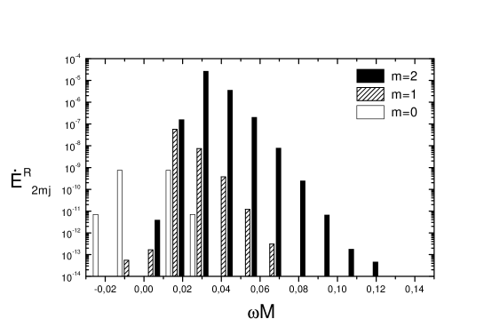
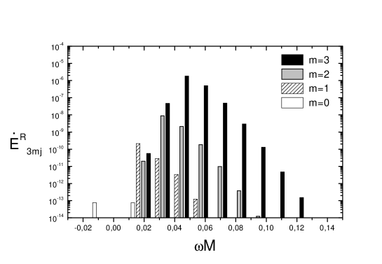
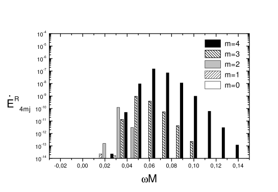
FIG. 1.: The gravitational emission associated to an eccentric orbit with $e=0.1$ and $r_{P}=3R_{s},$ is illustrated by plotting the amplitude of the spectral lines versus the dimensionless frequency  $M\omega_{mj}.$  The radiation computed by the hybrid quadrupole approach  $\dot{E}^{Q}_{mj}$  (upper panel, left) has to be compared with that computed by the relativistic approach,  $\dot{E}^{R}_{lmj},$  for  $l=2$  (upper panel, right). In the lower panel we plot the relativistic $l=3$ and $l=4$ contributions.

FIG. 2.: The ratio of the total power emitted in the $l$-th multipole,  $\dot{E}^{R}_{l},$  to the total power emitted in $l=2$,  $\dot{E}^{R}_{2},$  is plotted as a function of $l$, for an orbit with $e=0.1$ and $p=15.64$ ($r_{P}=3~{}R_{s}$). It clearly shows a power law behaviour  $\dot{E}^{R}_{l}\sim p^{l-2}.$  

FIG. 3.: In this figure we show how the spectral content of the gravitational emission changes as a function of the eccentricity, plotting the spectral lines  $\dot{E}^{R}_{lmj}$  as a function of the dimensionless frequency  $M\omega_{mj},$  for $l=m=2$ and for the same value of the periastron $r_{P}=3~{}R_{s}$. As the eccentricity increases, the location of the highest line shifts slightly towards a lower frequency, and higher order harmonics become more relevant.

FIG. 4.: The relative difference between the total power $\dot{E}^{Q}$ computed by the hybrid quadrupole approximation, and the total power emitted in the $l=2$ multipole, $\dot{E}^{(R)}_{2}$, computed by the relativistic approach, is plotted for circular orbits as a function of the radius $r_{0}$ (given in units of the stellar radius). When the point mass moves on an orbit far from the star the two approaches give the same result; the quadrupole emission becomes significantly larger than $\dot{E}^{(R)}_{2}$ for  $r_{0}<10~{}R_{S}.$  

FIG. 5.: The spectral line emitted by the system when the point mass moves on a close circular orbit is compared to the same quantity computed by the hybrid quadrupole formalism. The relativistic line (in black) is much larger than the quadrupole one (in white), because the frequency of the quadrupole line coincides with that of the fundamental mode of the star,  $\omega_{f},$  and a mechanism of resonant excitation occurs (see text).

FIG. 6.: The  $h^{TT}_{+}$  component of the gravitational wave emitted when the point mass moves on a circular orbit with  $r_{0}=3~{}R_{s},$  is plotted versus the retarded time in units of the orbital period. Since we assume that the observer is on the equatorial plane, the  $h^{TT}_{\times}$  component vanishes. In order to compare the relativistic waveform (continuous line) with the waveform computed by the hybrid quadrupole approach (dashed line), only the $l=2$ component of the relativistic signal is shown. The difference between the two signals is basically due to the $m=1$ contribution of the axial perturbations to the relativistic waveform (see text).

FIG. 7.: As in figure 6, we plot the  $h^{TT}_{+}$  component of the gravitational wave emitted when the point mass moves on an eccentric orbit with  $e=0.4$  and  $r_{P}=3R_{s}.$  The structure of the waveform is now much more complicated, but the beating of the frequencies induced by the $m=1$ axial contribution is still present.

REFERENCES

• [1] K. Oohara, T.Nakamura, Prog. Theor. Phys. Suppl. 136 , 270, (1999); M. Ruffert, H.T. Janka, Prog. Theor. Phys. Suppl. 136 , 287, (1999) ; F.A. Rasio, S.L. Shapiro, Class. Quant. Grav. 16, 1, (1999); T.W. Baumgarte, S.A. Hughes, S.L. Shapiro, Phys. Rev. D 60, 87501, (1999); M. Shibata, T.W. Baumgarte, S.L. Shapiro, Ap. J. 542, 453, (2000); K. Uryu, M. Shibata, Y. Eriguchi, Phys. Rev. D 62, 104015, (2000); J.A. Faber, F.A. Rasio, J.B. Manor, Phys. Rev. D 63, 044012, (2001)
• [2] V. Ferrari, L. Gualtieri, and A. Borrelli, Phys. Rev. D 59, 124020 (1999)
• [3] S.Chandrasekhar, V.Ferrari, Proc. R. Soc. Lond. A432, 247 (1990)
• [4] J.F. Zerilli, Phys. Rev D. 2, 2141 (1970)
• [5] T.Regge, J.A.Wheeler, Phys. Rev. 108, 1063 (1957)
• [6] M. Sasaki, T. Nakamura, Phys. Lett. 87A, 85 (1981)
• [7] J.M.Bardeen, W.H.Press, J. Math. Phys. 14, 7 (1973)
• [8] S.A.Teukolsky, Ap. J. 185, 635 (1973)
• [9] Y. Kojima, Prog. Theor. Phys. 77, 297, (1987).
• [10] J. Ruoff, P. Laguna, J. Pullin, Phys. Rev. D 63, 064019 (2001)
• [11] S.L.Detweiler, Ap. J 225, 687 (1978)
• [12] T.Nakamura, K. Oohara, Y. Kojima, Prog. Theor. Phys. Suppl. 90, 1 (1987)
• [13] V. Ferrari, K.D. Kokkotas, Phys. Rev. D 62, 107504 (2000)
• [14] E. Poisson, Phys. Rev. D 47, 1497 (1993)
• [15] C. Cutler, D. Kennefick, E. Poisson, Phys. Rev. D 50, 3816 (1994)
• [16] E. Berti, V. Ferrari, Phys. Rev. D 63, 064031 (2001)
• [17] T. Damour, B. R. Iyer, B.S. Sathyaprakash, Phys. Rev. D 57, 885 (1998)