Abstract

Gravitational waves are generated during first-order phase transitions, either by turbolence or by bubble collisions. If the transition takes place at temperatures of the order of the electroweak scale, the frequency of these gravitational waves is today just within the band of the planned space interferometer LISA. We present a detailed analysis of the production of gravitational waves during an electroweak phase transition in different supersymmetric models where, contrary to the case of the Standard Model, the transition can be first order. We find that the stochastic background of gravitational waves generated by bubble nucleation can reach a maximum value $h_{0}^{2}\Omega_{\rm gw}$ of order $(10^{-10}-10^{-11})$, which is within the reach of the planned sensitivity of LISA, while turbolence can even produce signals at the level $h_{0}^{2}\Omega_{\rm gw}\sim 10^{-9}$. These values of $h_{0}^{2}\Omega_{\rm gw}$ are obtained in the regions of the parameter space which can account for the generation of the baryon asymmetry at the electroweak scale.

PACS: 98.80.Cq; UGVA-DPT 07-1096; gr-qc/0107033

Introduction

Gravitational wave (GW) interferometers are presently under construction, and have as a possible target a stochastic background of GWs of cosmological origin (for reviews, see [1, 2, 3, 4]). In particular, the space interferometer LISA is expected to fly around 2010, with an extremely good sensitivity for GWs with a frequency $f$ between $10^{-4}$ Hz and 1 Hz [5]. It is quite fortunate that this is exactly the frequency range that a gravitational wave produced at a temperature $T\sim$ 100 GeV has today, after redshifting, and it is therefore interesting to investigate the intensity of GW backgrounds produced at a possible electroweak phase transition, and to compare it with the expected sensitivity of LISA.

Two main production mechanisms have been proposed for a first order phase transition: the first is the nucleation and collision of true vacuum bubbles [6, 7, 8, 9, 10, 11, 12]. The second is the onset of turbolence as a consequence of the injection of energy into the primordial plasma [12, 13].

These mechanisms are only effective for a strongly first order phase transition. For the Standard Model, the strength of the electroweak transition depends of the Higgs and $W$ masses, and can be investigate perturbatively only if $m_{H}\ll m_{W}$. The physical situation $m_{H}>m_{W}$ requires instead non-perturbative lattice computations, which have shown [14] that unfortunately there is no phase transition at all, but rather a smooth crossover. Therefore, in the Standard Model, no GWs are produced by this mechanism.

The strength of phase transitions, however, is strongly model- and parameter-dependent (for review, see [15]), and it is therefore meaningful to investigate whether in extensions of the Standard Model one can have a background of interest for LISA. In this paper we investigate the production of GWs in supersymmetric extensions of the SM. The strength of the phase transition has been investigated in connection with the generation of the baryon asymmetry [16], and it is known that in the Minimal Supersymmetric Standard Model (MSSM) a strong enough phase transition requires light Higgs and stop eigenstates [17]. If the Higgs is heavier than about 115 GeV, stronger constraints are imposed on the space of supersymmetric parameters. If one goes beyond the MSSM, introducing an additional gauge singlet in the Higgs sector (the so-called next-to-minimal SSM), it is known that the strength of the transition can be further enhanced [18].

The paper is organized as follows. In section 1 we review the physical processes that can lead to a stochastic background of gravitational waves during a phase transition; in particular, in section 1.3 we describe the strategy of our computation. Sections II and III are dedicated to the analysis of GW production, from turbolence and from bubble collisions, in two specific supersymmetric models: the Minimal Supersymmetric Standard Model (MSSM) and the Next-to-Minimal Supersymmetric Standard Model (NMSSM); we present a detailed analysis that extends results already reported in [19]. Our conclusions are presented in section IV.

1 GW production at phase transition

1.1 GW background from bubble collision

In first order phase transitions the Universe finds itself in a metastable state, which is separated from the true vacuum by a barrier in the potential of the order parameter, usually a scalar field $\phi$. True vacuum bubbles are then nucleated via quantum tunneling. In strongly first order phase transition the subsequent bubble dynamics is relatively simple: once the bubbles are nucleated, if they are smaller than a critical size their volume energy cannot overcome the shrinking effect of the surface tension, and they disappear. However, as the temperature drops below a critical temperature $T_{c}$, it becomes possible to nucleate bubbles that are larger than this critical size. These ‘critical bubbles’ start expanding, until their wall move at a speed close to the speed of light. The energy gained in the transition from the metastable state to the ground state is transferred to the kinetic energy of the bubble wall. As the bubble expands, more and more regions of space convert to the ground state, and the wall becomes more and more energetic. At the same time, it also becomes thinner, and therefore the energy density stored in the wall increases very fast. As long as we have a single spherical bubble, this large energy of course cannot be converted in GWs. But when two bubbles collide spherical symmetry is broken and we have the condition for the liberation of a large amount of energy into GWs. In particular, there are two possible ‘combustion’ modes for the two bubbles: detonation [20], that basically takes place when the boundaries propagate faster than the speed of sound, and deflagration, when instead they move slower. In the first case there is a large production of GWs [7, 6, 12]. The dynamics of a particular phase transition is governed by the effective potential for the scalar field(s) driving the transition itself. Given this effective potential, two are the basic quantities which play a role in the determination of the GW background generated during a first-order phase transition, and in which all the relevant features of the potential are encoded. The parameter $\alpha$ gives a measure of the jump in the energy density experienced by the order parameter $\phi$ during the transition from the false to the true vacuum and it is the ratio between the false vacuum energy density and the energy density of the radiation at the transition temperature $T_{*}$. The parameter $\beta$ characterizes the bubble nucleation rate per unit volume, which can be expressed as $\Gamma=\Gamma_{0}\exp(\beta t)$ [10]. Thus $\beta^{-1}=\Gamma/\dot{\Gamma}$ represents roughly the duration of the phase transition and the characteristic frequency of the gravitational radiation at time of production is expected to be $2\pi f\simeq\beta$. The stronger is the transition, the larger is $\alpha$ and the smaller is $\beta$ because of the larger amount of supercooling experienced by the system before the transition.
Once one has determined $\alpha$ and $\beta$, the gravitational radiation resulting from bubbles collisions can be calculated, for a strongly first order transition and for detonation combustion mode, in function of these two parameter only. We refer the reader to Ref. [12] for a detailed derivation and we summarize here only the strategy. The stress-energy tensor for a bubble expanding as a detonation front at velocity $v$ and of size $R\sim\beta^{-1}v$ takes a simple form, its relevant part coming from the wall’s contribution only. Its amplitude is proportional only to the kinetic energy density of the wall, which is a fraction $\kappa$ of the energy gained in the transition, namely the false vacuum energy density $\epsilon$ times the bubble’s volume $R^{3}\sim(\beta^{-1}v)^{3}$. Then the energy radiated during the collision of two bubbles is calculated from their stress-energy tensors using the envelope approximations, while the theory of relativistic combustion supported by numerical calculations gives $\kappa$ and $v$ as a function of $\alpha$. Taking in account the redshift from time of production up to now, and evaluating numerically the contribution from many randomly nucleated bubbles in a sample volume, one finally obtains the energy density of the radiation produced. It is convenient to express it in terms of the dimensionless quantity

$$h_{0}^{2}\Omega_{\rm gw}(f)=\frac{h_{0}^{2}}{\rho_{c}}\,\frac{d\rho_{\rm gw}}{d\log f}\,,$$ (1)

where $\rho_{\rm gw}$ is the energy density associated to GWs, $f$ is their frequency and $\rho_{c}$ is the present value of the critical energy density, $\rho_{c}=3H_{0}^{2}/(8\pi G_{N})$, with $H_{0}=100h_{0}$ Km/sec Mpc; $h_{0}$ parametrizes the uncertainty in $H_{0}$ (note that the combination $h_{0}^{2}\Omega_{\rm gw}$ is independent of $h_{0}$). LISA is expected to reach a sensitivity of order

$$h_{0}^{2}\Omega_{\rm gw}\simeq 10^{-12}\hskip 42.67912pt{\rm at}\,f=1\,{\rm mHz}\,.$$ (2)

At this frequency a cosmological signal could be masked by an astrophysical background due to unresolved compact white dwarf binaries. Its strength is uncertain, since it depends on the rate of white dwarf mergers and it is estimated to be [5]

$$h_{0}^{2}\Omega_{\rm gw}\simeq 10^{-11}\,.$$ (3)

At a frequency $f\simeq 10$ mHz the LISA sensitivity is expected to be of order $h_{0}^{2}\Omega_{\rm gw}\simeq 10^{-11}$, and the astrophysical background is expected to be below this value.

At the peak frequency $f_{\rm peak}$, the intensity $h_{0}^{2}\Omega_{\rm gw}$ of the radiation produced in bubble collisions is given, in terms of the parameters $\alpha$ and $\beta$ discussed above, by [12]

$$h_{0}^{2}\Omega_{\rm gw}\simeq 10^{-6}\left(\frac{0.7\>\alpha+0.2\sqrt{\alpha}}{1+0.7\>\alpha}\cdot\frac{\alpha}{1+\alpha}\right)^{2}\left(\frac{H_{*}}{\beta}\right)^{2}\left(\frac{v^{3}}{0.25+v^{3}}\right)\left(\frac{100}{g_{*}}\right)^{1/3}\,,$$ (4)

where $H_{*}$ and $g_{*}$ are respectively the Hubble parameter and the number of relativistic degrees of freedom at the time of transition and $v$ is the velocity at which the bubble expands. In the following we will use the value of the velocity $v=v(\alpha)$ as given in Ref. [12] for bubble detonation.

The detailed computations of $\alpha$ and $\beta$ will be the main issue of this paper. However, to have a first idea of the numbers involved, we note that early analytical estimates by Hogan [21, 7] indicated that it is difficult to obtain values of $H_{*}/\beta$ larger that ${\cal{O}}(10^{-2})$ (this estimate will be confirmed by our numerical results) and therefore, even for large values of $\alpha$, one should expect a signal at most of order $h_{0}^{2}\Omega_{\rm gw}\sim 10^{-10}$. This maximum value can be obtained only for strongly first order phase transition. The weaker the transition, the smaller are both $H_{*}/\beta$ and $\alpha$, and therefore we have further suppressions. It is clear that, since the value $h_{0}^{2}\Omega_{\rm gw}\sim 10^{-10}$ is already close to the limiting sensitivity of LISA, one can hope to find an observable signal only in some specific models, and in special regions of the parameter space; an observable signal will not be a generic property of extensions of the Standard Model. However, we know that the condition for strongly first order phase transition is the same that is required for producing the baryon asymmetry at the weak scale. Therefore the models and the regions of parameter space which produce an interesting GW signal, albeit quite specific, are also the most interesting if the baryon asymmetry has been indeed generated at the weak scale, and it makes sense to perform a detailed scanning of the parameter space in search of the strongest GW signal.

The present (i.e. properly red-shifted) peak frequency of the GW background is determined by $\beta$, by $H_{*}$, $g_{*}$, and by the transition temperature $T_{*}$ [12],

$$f_{\rm peak}\simeq 5.2\times 10^{-6}\>\left(\frac{\beta}{H_{*}}\right)\left(\frac{T_{*}}{100\>{\rm GeV}}\right)\left(\frac{g_{*}}{100}\right)^{1/6}\>{\rm Hz}\>.$$ (5)

At frequencies lower than $f_{\rm peak}$ the energy density increases like $f^{2.5}$, while above drops off more slowly [11]. As it will be shown in the following, typical values for $\beta/H_{*}$ for the electroweak phase transition are between $10^{2}$ and a few times $10^{3}$, with $T_{*}\sim 100$ GeV. This gives a frequency $f_{\rm peak}$ in the range $(10^{-4}-5\times 10^{-3})$ Hz, which is precisely the range in which LISA achieves its maximum sensitivity.

1.2 GW background from turbolence

During a first order transition there is another very general and possibly powerful source of gravitational waves. Part of the energy gained in the transition from the metastable state to the ground state is used to heat up the plasma, and another fraction is converted into bulk motion of the fluid. If the Reynolds number of the Universe at the phase transition is large enough, then this results in the onset of turbolence in the plasma, and consequently in the production of GWs. To compute accurately the amount of gravitational waves pruduced by turbolence is certainly a very difficult task. In the following, we will use the estimates for the characteristic frequency and for the intensity given in ref. [12],

$$f_{0}\simeq 2.6\times 10^{-6}\,{\rm Hz}\,\frac{v_{0}}{v}\left(\frac{\beta}{H_{*}}\right)\left(\frac{T_{*}}{100\>{\rm GeV}}\right)\left(\frac{g_{*}}{100}\right)^{1/6}$$ (6)

$$h_{0}^{2}\Omega_{\rm gw}\simeq 10^{-5}\left(\frac{H_{*}}{\beta}\right)^{2}vv_{0}^{6}\left(\frac{100}{g_{*}}\right)^{1/3}\;.$$ (7)

Here $v_{0}$ is the fluid velocity on the largest length scales on which the turbolence is being driven, and $v$ is again the velocity of the bubble wall. For a detonation, $v_{0}$ can be estimated to be $v_{0}\sim\sqrt{\kappa\alpha}$ for a weak transition (small $\alpha$) and $v_{0}\sim 1$ for a strong transition [12]. Strictly speaking, eq. (7) is derived in the regime of nonrelativistic fluid velocities (small $v_{0}$). A more detailed analysis of the GW production by turbolence has been recently announced as in preparation [13].

Substituting again typical $\beta/H_{*}$values of order $10^{2}-10^{3}$, and assuming large enough $v_{0}$ (detonation), we obtain a peak frequency around $10^{-4}-5\times 10^{-4}$ Hz, again well within the window of sensitivity of LISA. This is therefore another, very interesting, mechanism.

1.3 Computational method

Before analysing specific models, we describe how one can compute the relevant quantities appearing in Eqs. (4) and (5), namely $T_{*}$, $\alpha$ and $\beta/H_{*}$. We will perform a perturbative computation based on the thermal effective potential. This method is known to receive large non-perturbative corrections when the phase transition is radiatively induced [22, 23, 24, 25, 26]. In this case our results are really an upper bound on the GW production. However, the only situation in which we will find a signal compatible with LISA is when the potential has a metastable minimum already at tree level, and in this case our results are not expected to get important non-perturbative modifications.

The typical temperature dependence of a potential $V(\phi,T)$ for the Higgs scalar field(s), for a first-order transition, is shown in Fig. 1 (the figure refers for simplicity to one-dimensional potential, but the following discussion is valid also if several scalar fields are involved).

Figure 1: Typical temperature-dependence of the potential $V$ for a scalar field $\phi$ driving a first order transition. The dotted curve refers to very high temperature, while longer dashed lines refer to lower temperatures. $T_{1}$ is the temperature at which a minimum at $\langle\phi\rangle\neq 0$ develops; at $T_{\rm deg}$ the two minima are degenerate; at $T_{\rm dest}$ the origin $\langle\phi\rangle=0$ becomes unstable. The actual transition temperature $T_{*}$ is between $T_{\rm dest}$ and $T_{\rm deg}$.

In the case of a first order transition the rate of tunneling per unit volume $\Gamma$ from the metastable minimum to the stable one is in general suppressed by the exponential of an effective action, $\Gamma=\Gamma_{0}\;e^{-S}\;$ with

$$S=\int d\tau d^{3}x\left[\hbox{1000$\frac{1}{2}$}\left(\frac{d\phi}{d\tau}\right)^{2}+\hbox{1000$\frac{1}{2}$}(\vec{\nabla}\phi)^{2}+V(\phi)\right]\;,$$ (8)

where $\tau$ is the euclidean time. In the case of field theory at finite temperture $T$, one is led to consider Euclidean field theory periodic in imaginary time with period $T^{-1}$; moreover, in a cosmological context the temperature $T$ of the Universe decreases in time. Thus in our case the action (8) acquires a dependence on cosmic time $t$, and has to be computed in the space of functions periodic in Euclidean time $\tau$,

$$S(t)=\int_{0}^{\frac{1}{T}}\!d\tau d^{3}x\left[\hbox{1000$\frac{1}{2}$}\left(\frac{d\phi}{d\tau}\right)^{2}\!\!+\hbox{1000$\frac{1}{2}$}(\vec{\nabla}\phi)^{2}+V(\phi,T)\right]\;,$$ (9)

where $V(\phi,T)$ is the effective potential, shifted in such a way that $V(0,T)=0$. One then expands $S(t)$ around the transition time $t_{*}$, $S(t)\simeq S(t_{*})-\beta(t-t_{*})$ and identifies $\beta$ with $-(dS/dt)_{t_{*}}$. From $\Gamma\propto\exp(-S(t))$ it then follows that $\Gamma\propto\exp(\beta t)$. In a radiation dominated Universe this gives

$$\frac{\beta}{H_{*}}=\left.T_{*}\;\frac{d\left(S_{3}/T\right)}{dT}\right|_{T_{*}}\;,$$ (10)

where we have considered the large $T$ limit of (9) and have defined $S_{3}$ as the spatial Euclidean action

$$S_{3}(T)=\int d^{3}x\left[\hbox{1000$\frac{1}{2}$}(\vec{\nabla}\phi_{b})^{2}+V(\phi_{b},T)\right]$$ (11)

computed for the configuration of the scalar field(s) $\phi_{b}$ describing the bubble. The rate per unit volume of nucleation of a critical bubble is therefore

$$\Gamma=\Gamma_{0}\;\exp\left\{-\frac{S_{3}(T)}{T}\right\}\;,$$ (12)

where $\Gamma_{0}$ is of the order of $T^{4}$ for a finite temperature field theory.

The Euclidean action for a spherical configuration is

$$S_{3}(T)=4\pi\int dr\;r^{2}\left[\hbox{1000$\frac{1}{2}$}\left(\frac{d\,\phi_{b}}{d\,r}\right)^{2}+V(\phi_{b},T)\right]\;;$$ (13)

the bubble configuration is thus the solution of the equation(s)

$$\frac{d^{2}\phi_{b}}{dr^{2}}+\frac{2}{r}\frac{d\phi_{b}}{dr}-\frac{\partial V}{\partial\phi_{b}}=0$$ (14)

supplemented by the boundary conditions

$$\left.\frac{d\phi_{b}}{dr}\right|_{r=0}=0\>,\qquad\left.\phi_{b}\right|_{r=\infty}=0\;,$$ (15)

namely true vacuum inside the bubble and metastable vacuum outside. A typical bubble profile solution is shown in Fig. 2.

Figure 2: Typical profile of a bubble solution $\phi_{b}(r)$ interpolating from the true vacuum phase at $r=0$ to the false vacuum at $r=\infty$. The solution shown corresponds to the critical bubble at the transition temperature in the MSSM for $\sin^{2}\beta_{{\rm MSSM}}=0.8$, $m_{\rm Higgs}=110$ GeV and $m_{{\rm stop}}=140$ GeV, see section II.

In order to find the “escape point” (i.e. the value $\phi(r=0)\equiv\phi_{\rm e}$, implicitily determined by the two conditions (15)) one uses the “overshooting-undershooting” method illustrated in fig. 3. Equation (14) is the classical equation of motion for a point particle subject to a potential $-V(\phi)$ and to a velocity- and time-dependent friction force, if $\phi(r)$ stands for the trajectory of the particle. If the particle starts at rest precisely from the escape point, it will have just enough energy to overcome the friction force and to come at rest at $\phi=0$ at infinite $r$ (case (a)). If instead it starts at the right of $\phi_{\rm e}$ (overshooting), it will continue toward $\phi=-\infty$ (case (b)). If it starts at the left of $\phi_{\rm e}$ (case (c), undershooting) it will experience damped oscillation around the minimum of the inverted potential. Thus one determines the escape point by trials and errors, lowering the starting value if one gets a solution of type (b), and increasing it if one gets a solution of type (c). Once the escape point is found, the extremal action (13) can be computed for the corresponding solution.

       

Figure 3: Overshooting-undershooting method.

The bubble solution only exists in the range $T_{\rm dest}<T<T_{\rm deg}$, see fig. 1; for a one-dimensional potential the quantity $S_{3}(T)/T$ behaves as shown in fig. 4: at $T>T_{\rm deg}$ the transition cannot take place, because it is not energetically favorable to go from one minimum to the other, thus $S_{3}\to\infty$ and $\Gamma\to 0$. Conversely, for $T$ approaching $T_{\rm dest}$ the transition becomes more and more convenient, $S_{3}\to 0$ and $\Gamma\to\Gamma_{0}$.

Figure 4: The plot shows the rapid variation experienced by the action $S_{3}(T)/T$ (evaluated on critical bubble solutions) in a small range of temperature: $S_{3}(T)/T$ moves from 0 to $\infty$ going from $T=T_{\rm dest}$ to $T=T_{\rm deg}$, with $(T_{\rm deg}-T_{\rm dest})/T_{\rm dest}\sim 1\%$. The particular case shown in the figure refers to the electroweak transtion in the MSSM with $m_{\rm Higgs}=110$ GeV, $m_{{\rm stop}}=145$ GeV, $\sin^{2}\beta_{{\rm MSSM}}=0.8$, see section II.

The temperature $T_{*}$ at which the transition takes place is computed by comparing the probability of bubble nucleation per unit time and unit volume (12) with the expansion rate of the universe at the corresponding temperature. The condition that must be satisfied is that the probability for a single bubble to be nucleated within one horizon volume is ${\cal{O}}(1)$,

$$\int^{t_{*}}_{0}\frac{\Gamma}{H^{3}}dt=\int_{T_{*}}^{\infty}\frac{dT}{T}\left(\frac{90}{8\pi^{3}\>g}\right)^{2}\left(\frac{M_{\rm Pl}}{T}\right)^{4}e^{-S_{3}(T)/T}\sim 1\;.$$ (16)

For the electroweak transition, in which characteristic temperatures are ${\cal{O}}(100\>{\rm GeV})$, the condition above is well approximated by $S_{3}(T_{*})/T_{*}\simeq 140$.

Once one has found $T_{*}$, the parameter $\alpha$ is readily computed from the definition given above. Calling $v(T)$ the vacuum expectatuion value of the Higgs field at the true vacuum at temperature $T$, then the quantity

$$\epsilon_{*}=\left.-V(v(T),T)+T\frac{d}{dT}V(v(T),T)\right|_{T_{*}}$$ (17)

is the vacuum energy (latent heat) density associated with the transition (remember that the effective potential $V(\phi,T)$ is the free energy density). Thus $\alpha$ is the ratio between this and the energy density of the radiation,

$$\alpha=\frac{30\epsilon_{*}}{\pi^{2}g_{*}T_{*}^{4}}\;,$$ (18)

while $\beta/H_{*}$ is given by eq. (10). Notice that in order to compute $\alpha$ it is sufficient to know the transition temperature $T_{*}$ and the potential $V(\phi,T)$, while the determination of $\beta/H_{*}$ is possible only if one knows how the action $S_{3}(T)$ computed on the exact bubble solutions depends on $T$ in a neighbourhood of $T_{*}$.

2 The Minimal SuperSymmetric Standard Model

As we have already noticed, extensions of the SM are required to obtain a first-order phase transition at the electroweak scale, because in the SM, in the physical case $m_{\rm Higgs}>m_{W}$, there is no phase transition.

The Higgs sector of the MSSM requires two complex Higgs doublets, with opposite hypercharges

$$H_{1}=\left(\begin{array}[]{c}H_{1}^{0}\\ H_{1}^{-}\end{array}\right)_{-1/2}\;,\qquad H_{2}=\left(\begin{array}[]{c}H_{2}^{+}\\ H_{2}^{0}\end{array}\right)_{1/2}\;.$$ (19)

The tree-level potential is

$$V^{(0)}=m_{1}^{2}H_{1}^{\dagger}H_{1}+m_{2}^{2}H_{2}^{\dagger}H_{2}+m_{3}^{2}(H_{1}H_{2}+{\rm h.c.})+\frac{1}{8}g^{2}\left(H_{2}^{\dagger}\vec{\sigma}H_{2}+H_{1}^{\dagger}\vec{\sigma}H_{1}\right)^{2}+\frac{1}{8}g^{\prime 2}\left(H_{2}^{\dagger}H_{2}-H_{1}^{\dagger}H_{1}\right)^{2}$$ (20)

where the products between doublets are the usual SU(2) invariant products, the $\sigma_{i}$ are the Pauli matrices, $g$ and $g^{\prime}$ are the gauge couplings and the $m_{i}^{2}$ are real parameters, not necessarily positive. In fact, in order to have the gauge group SU(2)$\times$U(1) broken at zero temperature, one needs the quadratic term to be negative along some directions in the Higgs fields space.

We define $v_{1}=\langle H_{1}^{0}\rangle$, $v_{2}=\langle H_{2}^{0}\rangle$ and $\tan\beta_{\rm MSSM}=v_{2}/v_{1}$. In the following we will indicate the angle $\beta_{\rm MSSM}$ simply by $\beta$: it should not be confused with the parameter $\beta$ discussed in the previous sections that sets the time scale of phase transition.
As usual, the $W$ mass fixes $v^{2}\equiv v_{1}^{2}+v_{2}^{2}$ to the value $(246\;{\rm GeV})^{2}$. If the mass $m_{A}$ of the CP-odd field in the Higgs sector is much larger than $m_{W}$, only one light Higgs scalar $\phi$ is left and its tree-level potential is identical to the one in the SM, namely $V_{0}(\phi)=-\frac{m^{2}}{2}\phi^{2}+\frac{\lambda}{8}\phi^{4}$. This will be the case considered in this section. When $m_{A}\sim m_{W}$ the full two-Higgs potential should be considered, but the strength of the phase transition is weakened [17]. As we will see in the following, the one-loop thermal corrections to the effective potential make the quadratic term positive at high temperature and create a negative cubic term due to loops of the massive bosons in the theory. Due to the presence of this cubic term and the positivity of the quadratic one, there exists a range of temperature in which the point $\phi=0$ is a local minimum separated from the true simmetry-breaking one by a small potential barrier, that is precisely the set-up for a first-order phase transition. The strength of the phase transition is enhanced by the presence of new bosons coupled to the Higgs, a significant role being played by the right-handed stop $\;\widetilde{t}_{R}$, which is – apart from the Higgs itself – the lightest scalar in the theory and has the largest Yukawa coupling to the Higgs $\phi$.

To study the amount of gravitational waves generated during the electroweak phase transition within the MSSM we have made use of the thermal potential corrected up to two-loop level [29]. However, as discussed above, in this radiatively induced case, non-perturbative effects are also important. The results of ref. [24] indicate that the two-loop perturbative computation overestimates the amount of supercooling, so that the results of this section are really upper bounds on the GW production.

Following [29], we summarize here the one and two-loop finite temperature contributions to the effective potential for the Higgs field $\phi$. At one loop, the dominant corrections come from the gauge bosons $Z$ and $W$, the top quark and its supersymmetric partners. We will work in the limit in which the left handed stop is heavy, $m_{Q}\stackrel{{\scriptstyle>}}{{{}_{\sim}}}500$ GeV; lower values of $m_{Q}$ make the phase transition stronger, but give large contribution to the $\rho$-parameter. For right-handed stop masses below (or of order of) the top quark mass, and for large values of the CP-odd Higgs mass, $m_{A}\gg m_{Z}$, the one-loop effective potential admits the high temperature expansion [29]

$$V_{0}(\phi)+V_{1}(\phi,T)=-\frac{m^{2}(T)}{2}\phi^{2}+\frac{\lambda(T)}{8}\phi^{4}-T\left[E_{\rm SM}\;\phi^{3}+(2N_{c})\frac{\left(m_{\rm stop}^{2}(\phi)+\Pi_{\rm stop}(T)\right)^{3/2}}{12\pi}\right]\;,$$ (21)

where the various quantities are defined as follows: $N_{c}=3$ is the number of colors; $E_{\rm SM}$ is the cubic term coefficient in the Standard Model case,

$$E_{\rm SM}\simeq\frac{1}{3}\ \left(\frac{2m_{W}^{3}+m_{Z}^{3}}{2\pi v^{3}}\right)\;,$$ (22)

with $m_{W}$ and $m_{Z}$ standing for the physical masses of the gauge bosons at zero temperature. Here $m_{\rm stop}(\phi)$ is the lightest stop mass, which depends explicitely on the VEV of the Higgs $\phi$ and is approximately given by

$$m_{\rm stop}^{2}(\phi)\simeq m_{U}^{2}+\left[0.15\frac{m_{Z}^{2}}{v^{2}}\cos 2\beta+\frac{m_{t}^{2}}{v^{2}}\left(1-\frac{\tilde{A}_{t}^{2}}{m_{Q}^{2}}\right)\right]\phi^{2}\;,$$ (23)

where $m_{t}$ is the zero-temperature top quark mass, $m_{U}^{2}$ is a parameter of the model – the soft mass squared, not necessarily positive – and $\tilde{A}_{t}$ is the stop mixing parameter (which for simplicity will be set to zero in our numerical analysis). Here $\Pi_{\rm stop}(T)$ is the finite temperature contribution to the right-handed stop self-energy,

$$\Pi_{\rm stop}(T)=\frac{4}{9}g_{s}^{2}T^{2}+\frac{1}{6}h_{t}^{2}\left[1+\sin^{2}\beta\left(1-\widetilde{A}_{t}^{2}/m_{Q}^{2}\right)\right]T^{2}+\left(\frac{1}{3}-\frac{1}{18}|\cos 2\beta|\right)g^{\prime 2}T^{2}\;,$$ (24)

where $g_{s}$ is the strong gauge coupling and $h_{t}$ is the top Yukawa coupling; in our notations $m_{t}=h_{t}v\sin\beta/\sqrt{2}$. Finally $m^{2}(T)$ is given by

$$\frac{1}{2}m_{\rm Higgs}^{2}+\frac{T^{2}}{v^{2}}\left(\frac{1}{4}m_{\rm Higgs}^{2}+\frac{5}{6}m_{W}^{2}+\frac{5}{12}m_{W}^{2}+m_{t}^{2}\right)$$ (25)

and $\lambda(T)\simeq m_{\rm Higgs}^{2}/v^{2}$ apart from logarithmic corrections. As was observed in Ref. [30], the phase transition strength is maximized for values of the soft breaking parameter $m_{U}^{2}\simeq-\Pi_{\rm stop}(T)$, for which the coefficient of the cubic term in the effective potential,

$$E\simeq E_{\rm SM}+\frac{h_{t}^{3}\sin^{3}\beta\left(1-\widetilde{A}_{t}^{2}/m_{Q}^{2}\right)^{3/2}}{4\sqrt{2}\pi},$$ (26)

which governs the strength of the phase transition (in this case $v(T_{*})/T_{*}\simeq 4E/\lambda$), can be one order of magnitude larger than $E_{\rm SM}$ [30]. However, it was also noticed that such large negative values of $m_{U}^{2}$ may induce the presence of color breaking minima because the effective stop mass at finite temperature $m^{2}_{\rm stop}(\phi)+\Pi_{\rm stop}(T)$ may become negative [33, 30]. The problem arises for small values of the VEV of $\phi$ and of the temperature $T$, as one can easily infer from Eqs. (23) and (24). Thus, the check one has to perform is that for $T>T_{*}$ – i.e. before the phase transition takes place – the sum $m^{2}_{\rm stop}(\langle\phi\rangle)+\Pi_{\rm stop}(T)=m_{U}^{2}+\Pi_{\rm stop}(T)$ is positive, the equality being motivated by the fact that $\langle\phi\rangle=0$ for $T>T_{*}$. Once the above condition is satisfied, the color breaking minima problem is absent for $T<T_{*}$ too, because the VEV $\langle\phi\rangle$ gets a large value ${\cal{O}}(100\>{\rm GeV})$ after the phase transition.

Before performing the full computation with the two-loop corrections to the potential, we proceed to a rough computation of the quantity $\alpha$ defined in section 1.1, using the one-loop effective potential (21), in order to understand the dependence of the strength of the phase transition on the various parameters of the model, and to identify the regions of the parameter space where it is appropriate to perform more detailed computations.

Under the assumptions mentioned above, the most relevant parameters in the game are the Higgs mass $m_{\rm Higgs}$, the right-handed stop mass $m_{\rm stop}$ and the zero temperature ratio between the vacuum expectation values of the two neutral Higgses $\tan\beta$. However, it is well known that the strength of the transition has a very slight dependence on $\tan\beta$, with slightly stronger transition at high (i.e. greater than about 0.6) values of $\sin^{2}\beta$. In our computations we will set both $\sin^{2}\beta=0.8$ and $\sin^{2}\beta=0.3$, obtaining very similar results. Our strategy has been the following. For every value of $m_{\rm Higgs}$ and $m_{\rm stop}$ we computed the temperature $T_{\rm dest}$ at which the origin $\phi=0$ gets destabilized; then we computed $\alpha$ setting $T_{*}=T_{\rm dest}$ in the definition (18). The actual temperature $T_{*}$ is in the range between the “destabilization temperature” $T_{\rm dest}$ and the “degeneracy temperature” $T_{\rm deg}$, as discussed in section 1.3. For the model under study this range is very small, $(T_{\rm deg}-T_{\rm dest})/T_{\rm dest}\sim(1-3)\,\%$. So even taking $T_{*}$ to be equal to $T_{\rm dest}$ leads nevertheless to the right order of magnitude in the calculation of the parameter $\alpha$. Our results are summarized in figs. 5 and 6, which show contour plots for $\alpha$ as a function of $m_{\rm Higgs}$ and $m_{\rm stop}$, together with the region forbidden by the condition of absence of color breaking minima discussed above.

Figure 5: Contour plot of $\alpha$ as a function of the Higgs and stop masses for $\sin^{2}\beta=0.8$. The shaded region is forbidden by the request of absence of color breaking minima. $\alpha$ is computed at the destabilization temperature, as discussed in the text.                       

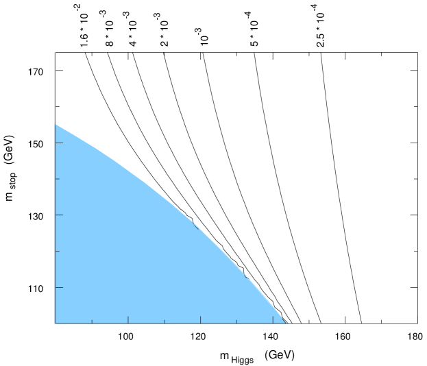
Figure 6: Contour plot of $\alpha$ as a function of the Higgs and stop masses for $\sin^{2}\beta=0.3$ .

From figs. 5 and 6 we see that in order to have large values for $\alpha$ one needs small Higgs and stop masses; this agrees with the well known fact that the strength of the electroweak transition is enhanced by taking light Higgs and stop. We see also that the strength of the transition is very slightly dependent on $\sin^{2}\beta$; thus for definiteness we fix $\sin^{2}\beta=0.8$.

The most important two loop corrections are of the form $\phi^{2}\log(\phi)$ and are induced by the Standard Model weak gauge bosons as well as by the stop and gluon loops [28, 31]

$$V_{2}(\phi,T)\simeq\frac{\phi^{2}T^{2}}{32\pi^{2}}\left[\frac{51}{16}g^{2}-3h_{t}^{4}\sin^{4}\beta\left(1-\frac{\widetilde{A}_{t}^{2}}{m_{Q}^{2}}\right)^{2}+8g_{s}^{2}h_{t}^{2}\sin^{2}\beta\left(1-\frac{\widetilde{A}_{t}^{2}}{m_{Q}^{2}}\right)\right]\log\left(\frac{\Lambda_{H}}{\phi}\right)$$ (27)

where the first term comes from the Standard Model gauge boson-loop contributions, while the second and third terms come from the light supersymmetric particle loop contributions. The scale $\Lambda_{H}$ depends on the finite corrections [28] and is of order of 100 GeV: given the slight logarithmic dependence of $V_{2}$ on $\Lambda_{H}$, in the following we will set $\Lambda_{H}=100$ GeV. The complete potential we use is thus $V(\phi,T)=V_{0}(\phi)+V_{1}(\phi,T)+V_{2}(\phi,T)$.

Next, having fig. 5 in mind, we proceeded to an accurate numerical computation of the parameters $\alpha$ and $\beta/H_{*}$ characterizing the strength of the phase transition: for any given choice of the masses $m_{\rm Higgs}$ and $m_{\rm stop}$, we have first numerically computed the nucleation temperature $T_{*}$ by imposing that, for the Higgs field configuration describing the nucleated bubble, the condition $S_{3}(T_{*})/T_{*}\simeq 140$ is satisfied. Then we have computed the parameters $\alpha$ and $\beta/H_{*}$ through Eqs. (18) e (10). Our results are summarized in Figs. 7 and 8.

Figure 7: Plot for $\alpha$ (dashed line), $\beta/H_{*}$ (dotted line), and $h_{0}^{2}\Omega_{\rm gw}$ from bubble collisions (solid line), as functions of the stop mass, for a 110 GeV Higgs and $\sin^{2}\beta=0.8$.

The intensity of the produced gravity waves rapidly grows as the masses decrease. This is explained by the fact that $h_{0}^{2}\Omega_{\rm gw}$ scales roughly as $\alpha^{3}/\beta^{2}$ and a linear increase of $\alpha$ and decrease of $\beta$ leads to a rapid power-law growth of the intensity. Unfortunately, the general prediction is that the intensity of the gravitational waves produced during the MSSM phase transition is too small for LISA. For instance, taking a Higgs mass of 110 GeV, the right-handed stop mass of 140 GeV and $\sin^{2}\beta=0.8$ (see fig. 7), we find $\alpha\simeq 3\times 10^{-2}$ and $\beta/H_{*}$$\simeq 4\times 10^{3}$, leading to $h_{0}^{2}\Omega_{\rm gw}\simeq 2\times 10^{-18}$. Notice that one is not allowed to lower too much the right-handed stop mass because of the problem of color breaking minima described above.

Figure 8: Plot for $\alpha$ (dashed line), $\beta/H_{*}$ (dotted line), and $h_{0}^{2}\Omega_{\rm gw}$ from bubble collisions (solid line), as functions of the Higgs mass, for a 155 GeV stop and $\sin^{2}\beta=0.8$.

We have also estimated what happens if we lower the Higgs mass down to (the already excluded value of) 80 GeV, setting the right-handed stop mass at 155 GeV – which is the lower value compatible with the absence of color breaking minima – and $\sin^{2}\beta=0.8$, see fig. 8. We obtain $\alpha\simeq 0.1$ and $\beta/H_{*}$$\simeq 2\times 10^{3}$, giving $h_{0}^{2}\Omega_{\rm gw}\simeq 2\times 10^{-16}$, a signal still not relevant. The situation does not improve when both Higgses are involved in the transition because the strength of the phase transition is weaker. An uncertainty in this estimate is due to the determination of $v$, the velocity of expansion of the bubble discussed in section 1.1. If the phase transition is not strong enough, then $v$ is subsonic, so that the value of $h_{0}^{2}\Omega_{\rm gw}$ is further suppressed.

It is now easy to estimate also the amount of GWs produced by turbolence at the electroweak transition, in the MSSM case. Substituting in eq. (7) tha values of $\alpha$ and $\beta/H_{*}$ found above, we obtain the plots shown in figs. 9 and 10. Again, the results are too small to be of interest for LISA.

Figure 9: $h_{0}^{2}\Omega_{\rm gw}$ from turbolence, as a function of the stop mass for a 110 GeV Higgs and $\sin^{2}\beta=0.8$.

Figure 10: $h_{0}^{2}\Omega_{\rm gw}$ from turbolence, as a function of the Higgs mass for a 155 GeV stop and $\sin^{2}\beta=0.8$.

3 The Next-to-Minimal Supersymmetric Standard Model

3.1 The model

The situation improves considerably if we enlarge the MSSM sector adding a complex gauge singlet $N$ [27]. This is the so-called Next-to-Minimal Supersymmetric Standard Model (NMSSM) and is a particularly attractive model to explain the observed baryon asymmetry at the electroweak phase transition. The relevant part of the superpotential is given by

$$W=\lambda H_{1}H_{2}N-\frac{k}{3}N^{3}\;,$$

where now the supersymmetric $\mu$-parameter of the MSSM is substituted by the the combination $\lambda\langle N\rangle$, and $k$ is a free parameter. The corresponding tree level Higgs potential reads $V=V_{F}+V_{D}+V_{{\rm soft}}$, where

$$V_{F} = |\lambda|^{2}\left[|N|^{2}(|H_{1}|^{2}+|H_{2}|^{2})+|H_{1}H_{2}|^{2}\right]+k^{2}|N|^{4}-(\lambda k^{*}H_{1}H_{2}{N^{2}}^{*}+{\rm h.c.})$$ (28)

$$V_{D} = \frac{g^{2}+g^{\prime 2}}{8}(|H_{2}|^{2}-|H_{1}|^{2})^{2}+\frac{g^{2}}{2}|H_{1}^{{\dagger}}H_{2}|^{2}$$ (29)

$$V_{{\rm soft}} = m_{H_{1}}^{2}|H_{1}|^{2}+m_{H_{2}}^{2}|H_{2}|^{2}+m_{N}^{2}|N|^{2}-\left(\lambda A_{\lambda}H_{1}H_{2}N-\frac{1}{3}kA_{k}N^{3}+{\rm h.c.}\right)\;.$$ (30)

The presence of the cubic supersymmetry breaking soft terms proportional to the parameters $A_{\lambda}$ and $A_{k}$ already at zero temperature makes it clear that within the NMSSM it is quite easy to get a very strong first-order phase transition at the electroweak scale [18]. The order of the transition is determined by these trilinear soft terms rather than by the cubic term appearing in the finite temperature one-loop corrections and the preservation of baryon asymmetry after the phase transition is possible for masses of the lightest scalar up to about 170 GeV. At the same time, since the transition is induced by the tree-level terms rather than by radiative corrections, non-perturbative effects are non expected to change dramatically the results of the perturbative computation.

By a redefinition of the global phases of $H_{1}$ and $N$ it is always possible to take $\lambda A_{\lambda}$ and $kA_{k}$ real and positive, while by an SU(2)$\times$U(1) global rotation one can put $v^{\pm}\equiv\langle H^{\pm}\rangle=0$ and $v_{2}\equiv\langle H_{2}^{0}\rangle\in R^{+}$. Assuming CP conservation, also $v_{1}^{0}\equiv\langle H_{1}\rangle$ and $x\equiv\langle N\rangle$ are real.

Before introducing finite temperature corrections, we summarize here some aspects of the tree level potential. First, it contains seven free parameters, but imposing the stationarity conditions in $(H_{1}^{0},H_{2}^{0},N)=(v_{1},v_{2},x)$ with the constraint $v_{1}^{2}+v_{2}^{2}\equiv v^{2}=(246\;{\rm GeV})^{2}$ , we can express the soft masses in terms of the six parameters $\lambda$, $k$, $A_{\lambda}$, $A_{k}$, $\tan\beta$ and $x$,

$$m_{H_{1}}^{2} = \lambda(A_{\lambda}+kx)x\tan\beta-\lambda^{2}(x^{2}+v^{2}\sin^{2}\beta)-\frac{g^{2}+g^{\prime 2}}{4}v^{2}\cos 2\beta$$

$$m_{H_{2}}^{2} = \lambda(A_{\lambda}+kx)\,x\,{\rm cotan}\beta-\lambda^{2}(x^{2}+v^{2}\cos^{2}\beta)+\frac{g^{2}+g^{\prime 2}}{4}v^{2}\cos 2\beta$$ (31)

$$m_{N}^{2} = \lambda A_{\lambda}\frac{v^{2}}{2x}\sin 2\beta+kA_{k}x-\lambda^{2}v^{2}-2k^{2}x^{2}+\lambda kv^{2}\sin 2\beta\;.$$

The above equations do not guarantee that $(v_{1},v_{2},x)$ is the global minimum of the tree level potential: for each choice of the parameters we must verify that this is indeed the case.

Concerning the physical masses of the 6 physical Higgs fields, one has to consider the matrix of the second derivatives of the tree-level potential. In order to avoid the formation of dangerous directions of instability in the space of charged and pseudoscalar Higgses, in the analysis of the strength of the transition for each choice of the parameters one has to verify the positiveness of their mass matrixes.

Finally, barring the possibility that the transition occurs along CP-violating directions, the potential becomes a function of three real scalar fields only, $({\rm Re}H_{1}^{0},{\rm Re}H_{2}^{0},{\rm Re}N)$ which in the following will be denoted by $(\phi_{1},\phi_{2},\phi_{3})$.

In our numerical analysis we made use of the tree-level potential $V_{F}+V_{D}+V_{\rm soft}$, restricted to the three neutral scalar fields left, plus the one-loop corrections appearing at finite temperature. Overall, we have six free parameters: the coupling parameters $\lambda$ and $k$; the soft-breaking mass terms $A_{\lambda}$ and $A_{k}$; the zero-temperature vacuum expectation value of the singlet $x$ and $\tan\beta$. The thermal corrections to the potential involve a linear term,

$$\frac{1}{8}T^{2}\sin(2\beta)\>\lambda A_{\lambda}\phi_{3}\;,$$ (32)

and a bilinear one,

$$\frac{T^{2}}{24}\left(C_{H_{1}}\>\phi_{1}^{2}+C_{H_{2}}\>\phi_{2}^{2}+C_{N}\>\phi_{3}^{2}+2C_{12}\>\phi_{1}\phi_{2}\right)\;,$$ (33)

where the $C$’s are constants depending on $\lambda$, $k$ and $\tan\beta$ [18].

3.2 The landscape of minima

Since we have now to deal with three scalars and six free parameters, the NMSSM case is considerably more complicated than the case of one light Higgs in the MSSM. Besides increased computational difficulty, new features arise.

First of all, the strength of the transition is dominated by the tree-level trilinear term rather than by loop corrections, and therefore it is not anymore directly related to the Higgses and stop masses (neither is related in a simple way to the six parameters of the tree level potential).

More in general, the landscape of local and global minima in this large parameter space is more complicated. Indeed, for some choices of the parameters the destabilization does not even take place, while for other values of the parameters, at $T=T_{\rm dest}$ the origin gets destabilized along a direction which does not connect the origin to the true vacuum, but to a local minimum, separated from the global one by a barrier: in these cases the system first rolls down to the new “shifted” false vacuum (second order transition), and next it tunnels through the barrier which separates it from the true vacuum (first order transition). These two minima are separated by a potential barrier in the three-dimensional field space ($\phi_{1},\phi_{2},\phi_{3}$); tunneling throughout the barrier will take place through the trajectory in this field space which leads to the least Euclidean action (13) and this in general will not be a straight line. Our approximation from now on is that this least-action trajectory is in fact a straight line joining the two minima: in other words, after having exactly computed the two minima, we reduce the problem to a one dimensional system along the direction joining these two points, thus simplifying the computation of bubble solutions. This perhaps leads to a small overestimate of the strength of the transition.

In our analysis we have focussed on those regions of the parameter space which previous studies have shown to give rise to a large baryon asymmetry; our strategy has been the following. First, we made a quicker scanning of wide regions in the six dimensional parameters space. At this stage, it would be highly impractical to reconstruct the bubble profile and compute $\alpha$ and $\beta$ for each value of the parameters explored; instead, in order to have an idea of what are the most interesting regions, we computed, at the degeneracy temperature and (if it exists) at the destabilization temperature, the height of the potential barrier and the energy density difference between the false vacuum (possibly shifted, as discussed above) and the true vacuum.

These first estimates allowed us to select the regions in the parameters space which present a strong phase transition; in particular, it turns out that the most important parameters in the game are the soft breaking mass terms $A_{\lambda}$ and $A_{k}$. We then moved to a more accurate analysis restricted to some of the interesting regions found.

The situation is now much more complicated than in the MSSM case, becuase of the higher dimensionality of the Higgs space. Furthermore, now the barrier is much higher than in the MSSM, and therefore the system has to experience an higher degree of supercooling before the transition can take place. Thus, while in the MSSM the separations between the temperature of degeneracy for the two vacua $T_{\rm deg}$, the actual transition temperature $T_{*}$, and the origin-destabilization temperature $T_{\rm dest}$, are of order of a few GeVs, in the NMSSM these intervals can be sensibly larger (and indeed, as discussed above, for some ranges of the parameters the destabilization can even be absent). This fact makes it harder the compute precisely the value transition temperature $T_{*}$, and thus of $\alpha$. In order to get a contour plot for the function $\alpha(A_{\lambda},A_{k})$ we proceeded as follows. The transition takes place when $S_{3}(T)/T\simeq 140$, $S_{3}$ being the sum of a kinetic term and a potential one (see (13)). These two terms are likely to be of the same order if evaluated on the bubble-like solution of the equations of motion, and thus $S_{3}(T)\propto\int\!dr\,r^{2}\,V(\phi_{b},T)$. The integral of the potential extended to the bubble receives a contribution mainly from the wall proportional to the maximum $V_{\rm max}$ of the potential and a contribution from the inside of the bubble proportional to the minimum $V_{\rm min}$, i.e. $S_{3}(T)\sim A\cdot V_{\rm max}(T)+B\cdot V_{\rm min}(T)$, with $A$ and $B$ depending on the exact solution $\phi_{b}(r)$. The condition to determine $T_{*}$ thus becomes $A\cdot V_{\rm max}(T_{*})+B\cdot V_{\rm min}(T_{*})\sim 140\,T_{*}$. We assumed constant $A$ and $B$ in each small region we explored, thus fitting their value with several exact solutions $\phi_{b}(r)$. As in the MSSM case, once this (approximate) transition temperature $T_{*}$ is evaluated, one easily computes $\alpha$ from its definition (18). A result of this procedure is summarized in fig. 11, which shows a rapid growth of $\alpha$ versus $A_{\lambda}$ and $A_{k}$, with $x=350$ GeV, $\lambda=0.83$, $k=0.67$ and $\tan\beta=2$.

Figure 11: Rough contour plot for $\alpha$ as a function of $A_{\lambda}$ and $A_{k}$, for $x=350$ GeV, $\lambda=0.83$, $k=0.67$ and $\tan\beta=2$ .

Next we moved to computing exactly $T_{*}$, $\alpha$ and $\beta/H_{*}$ for specific values of $A_{\lambda}$ and $A_{k}$ in the region of fig. 11, again by numerically computing the temperature for which the bubble solution $\phi_{b}(r)$ gives $S_{3}(T)/T\simeq 140$ and then applying relations (18) and (10). Typical results are shown in Figs. 12 and 14, where we plot $\alpha$, $\beta/H_{*}$ and $h_{0}^{2}\Omega_{\rm gw}$ as functions of $A_{\lambda}$ and $A_{k}$.

Note that, since the transition in the NMSSM is strongly first order, it is correct to use the expression for $v(\alpha)$ computed for detonation bubbles [12]. The results shown in the figures are not peculiar of the values of the parameters chosen: similar results can be found in completely different regions of the parameters space, see for instance fig. 16.

An example of a region of the parameter space in which the transition happens through the nucleation of bubbles subsequent to a smooth roll-down is shown in fig. 18.

Figure 12: Plot for $\alpha$ (dashed line), $\beta/H_{*}$ (dotted line), and $h_{0}^{2}\Omega_{\rm gw}$ (solid line) from bubble collisions, as functions of $A_{\lambda}$ for $A_{k}=480$ GeV, $x=350$ GeV, $\lambda=0.83$, $k=0.67$ and $\tan\beta=2$.

Figure 13: $h_{0}^{2}\Omega_{\rm gw}$ from turbolence as a function of $A_{\lambda}$ for $A_{k}=480$ GeV, $x=350$ GeV, $\lambda=0.83$, $k=0.67$ and $\tan\beta=2$.

Figure 14: Plot for $\alpha$ (dashed line), $\beta/H_{*}$ (dotted line), and $h_{0}^{2}\Omega_{\rm gw}$ (solid line) from bubble collisions, as functions of $A_{k}$ for $A_{\lambda}=450$ GeV, $x=350$ GeV, $\lambda=0.83$, $k=0.67$ and $\tan\beta=2$.

Figure 15: $h_{0}^{2}\Omega_{\rm gw}$ from turbolence as a function of $A_{k}$ for $A_{\lambda}=450$ GeV, $x=350$ GeV, $\lambda=0.83$, $k=0.67$ and $\tan\beta=2$.

Figure 16: Plot for $\alpha$ (dashed line), $\beta/H_{*}$ (dotted line), and $h_{0}^{2}\Omega_{\rm gw}$ from bubble collisions (solid line), as functions of $A_{\lambda}$ for $A_{k}=167$ GeV, $x=300$ GeV, $\lambda=0.523$, $k=0.37$ and $\tan\beta=2$.

Figure 17: $h_{0}^{2}\Omega_{\rm gw}$ from turbolence as a function of $A_{\lambda}$ for $A_{k}=167$ GeV, $x=300$ GeV, $\lambda=0.523$, $k=0.37$ and $\tan\beta=2$.

Figure 18: Plot for $\alpha$ (dashed line), $\beta/H_{*}$ (dotted line), and $h_{0}^{2}\Omega_{\rm gw}$ from bubble collisions, (solid line) as functions of $A_{k}$ for $A_{\lambda}=450$ GeV, $x=350$ GeV, $\lambda=0.83$, $k=0.67$ and $\tan\beta=2$.

Figure 19: $h_{0}^{2}\Omega_{\rm gw}$ from turbolence as a function of $A_{k}$ for $A_{\lambda}=450$ GeV, $x=350$ GeV, $\lambda=0.83$, $k=0.67$ and $\tan\beta=2$.

In figs. 16 and 14 the intensity of the produced gravity waves grows rapidly as a function of the soft breaking mass terms. However, $A_{\lambda}$ and $A_{k}$ cannot be extended beyond the values shown in the figures: beyond such values the condition $S_{3}(T_{*})/T_{*}\simeq 140$ is never satisfied and the transition does not take place. This is due to the presence of a potential barrier also at zero temperature, generated by trilinear terms in the tree-level potential: as discussed in section 1.3, the Euclidean action $S_{3}(T)$ computed on the bubble solution decreases from $+\infty$ to 0 in going from $T=T_{\rm deg}$ to $T=T_{\rm dest}$; if the origin never gets destabilized – as in the cases we are considering here – one has $S_{3}(T)\to{\rm const}\neq 0$ as $T\to 0$. The value of this constant is related to the heigth of the zero-temperature potential barrier, and it is possible that the quantity $S_{3}(T)/T$ never reaches the critical value $\simeq 140$. This behavior is illustrated in fig. 20  . It is clear that moving to these extreme regions makes $\beta/H_{*}$ close to zero, because it is proportional to the slope of $S_{3}/T$ computed at the “crossing” $S_{3}/T\simeq 140$ (see fig. 20). By physical reasons, one cannot accept values of $\beta/H_{*}$ smaller than 1: for such values the transition would be so slow that it doesn’t complete in a Hubble time, and clearly the computations that lead to (4) are not valid in such a case. Our best results give therefore values of $h_{0}^{2}\Omega_{\rm gw}\sim 10^{-10}$, peaked at a frequency, obtained from eq. 5, of approximately 10 mHz.

Figure 20: Behaviour of the action $S_{3}/T$ versus $T$ in an “extremal” region of the parameters-space. The horizontal dashed line indicates the value $S_{3}/T\simeq 140$ that must be reached in order that the transition takes place.

3.3 Gravitational waves from turbolence in the NMSSM

We now estimate the amount of GWs produced by turbolence in the case of the NMSSM for the specific regions of the parameter space studied in the previous section. Substituting in eq. (7) the values of $\alpha$ and $\beta/H_{*}$ shown in figs. 12, 14, 16 and 18 we obtain for $h_{0}^{2}\Omega_{\rm gw}$ the plots of figs. 13, 15, 17 and 19.

We recall again that, due to the difficulties in estimating accurately the production of GWs from turbolence, these plots should be taken only as indicative. Still, they suggest that turbolence can be a really powerful source of GWs, indeed more powerful than the better studied mechanism of bubble collisions. In special points of the parameter space, we find values of $h_{0}^{2}\Omega_{\rm gw}$ even of order $10^{-9}$, which would correspond to a signal-to-noise ratio of order 100 for LISA! It is clear that the production of GWs by turbolence deserves further studies.

4 Conclusions

The production of GWs at the electroweak scale is strongly dependent on the model used and on the parameters of the model. This is an expected consequence of the well known fact that the strength of the phase transition is itself strongly dependent. Our aim was to compare the production of GWs with the reference value given by the sensitivity of LISA. In the Standard Model, for the experimentally allowed values of the Higgs mass, there is no electroweak phase transition at all, and therefore no production of GWs. We have therefore turned our attention to supersymmetric extensions. For the MSSM the answer is again negative. The results never exceed values of order $h_{0}^{2}\Omega_{\rm gw}\sim 10^{-16}$, five orders of magnitudes below the sensitivity of LISA.

More encouraging results can be obtained in the Next-to-Minimal Supersymmetric Standard Model, basically because in this case the transition is due to tree level couplings, rather than being radiatively induced. In this case, while in many regions of the parameter space the signal is still neglegible, there are also region where one can get $h_{0}^{2}\Omega_{\rm gw}\sim 10^{-10}$ from bubble nucleation and even $h_{0}^{2}\Omega_{\rm gw}\sim 10^{-9}$ from turbolence, with a peak frequency around 10 mHz. A background of this intensity would be within the reach of LISA.

While regions of parameter space with such large values are, generically speaking, quite small, it must be observed that the condition for an intense GW production is the same as the condition for the generation of the baryon asymmetry at the electroweak scale.

References

- [1] K.S. Thorne, in 300 Years of Gravitation, S. Hawking and W. Israel eds., Cambridge U. P., Cambridge, 1987.
- [2] B. Allen, gr-qc/9604033.
- [3] M. Maggiore, Phys. Rept. 331, 283 (2000).
- [4] M. Maggiore, gr-qc/0008027.
- [5] K. Danzmann for the LISA study team, Class. Quant. Grav. 14 (1997) 1399; P. Bender et. al, LISA. Pre-Phase A Report, second edition, July 1998, available at http://www.lisa.uni-hannover.de/lisapub.html
- [6] E. Witten, Phys. Rev. D30 (1984) 272.
- [7] C. Hogan, Mon. Not. R. Astr. Soc. 218 (1986) 629.
- [8] M. Turner and F. Wilczek, Phys.Rev.Lett. 65(1990) 3080.
- [9] A. Kosowsky, M. S. Turner and R. Watkins, Phys. Rev. Lett. 69 (1992) 2026; Phys. Rev. D 45 (1992) 4514.
- [10] M. S. Turner, E. J. Weinberg and L. M. Widrow, Phys. Rev. D 46 (1992) 2384.
- [11] A.Kosowsky and M.Turner, Phys. Rev. D 47 (1993) 4372
- [12] M. Kamionkowski, A. Kosowsky and M. S. Turner, Phys. Rev. D 49 (1994) 2837
- [13] A. Kosowsky, A. Mack and T. Kahniashvili, astro-ph/0102169.
- [14] K. Kajantie, M. Laine, K. Rummukainen and M. Shaposhnikov, Phys. Rev. Lett. 77, 2887 (1996).
- [15] V. A. Rubakov and M. E. Shaposhnikov, Usp. Fiz. Nauk 166 (1996) 493 [Phys. Usp. 39 (1996) 461]
- [16] For a recent review, see A. Riotto and M. Trodden, Ann. Rev. Nucl. Part. Sci. 49, 35 (1999).
- [17] For a recent review, see M. Quiros, hep-ph/0101230.
- [18] M. Pietroni, Nucl. Phys. B402, 27 (1993); for a recent analysis, see S. J. Huber and M. G. Schmidt, hep-ph/0003122 and refs. therein.
- [19] R. Apreda, M. Maggiore, A. Nicolis and A. Riotto, hep-ph/0102140.
- [20] P. Steinhardt, Phys. Rev. D25 (1982) 2082.
- [21] C. Hogan, Phys. Lett. 133B (1983) 172.
- [22] A. Strumia and N. Tetradis, Nucl. Phys. B 554 (1999) 697
- [23] A. Strumia and N. Tetradis, JHEP 9911 (1999) 023
- [24] G. D. Moore and K. Rummukainen, Phys. Rev. D 63 (2001) 045002
- [25] G. D. Moore, K. Rummukainen and A. Tranberg, JHEP 0104 (2001) 017
- [26] G. Munster, A. Strumia and N. Tetradis, Phys. Lett. A 271 (2000) 80
- [27] J. Ellis, J. F. Gunion, H. E. Haber, L. Roszkowski and F. Zwirner, Phys. Rev. D 39, 844 (1989).
- [28] J. Bagnasco and M. Dine, Phys. Lett. B30393308; P. Arnold and O. Espinosa, Phys. Rev. D47933546; Z. Fodor and A. Hebecker, Nucl. Phys. B43294127
- [29] M. Carena, M. Quiros and C. E. Wagner, Nucl. Phys. B 524 (1998) 3 [hep-ph/9710401].
- [30] M. Carena, M. Quiros and C.E.M. Wagner, Phys. Lett. B3809681
- [31] J.R. Espinosa, Nucl. Phys. B47596273
- [32] D. Bodeker, P. John, M. Laine and M.G. Schmidt, Nucl. Phys. B49797387
- [33] M. Carena and C.E.M. Wagner, Nucl. Phys. B4529545