Signal recycled laser-interferometer gravitational-wave detectors as optical springs

Abstract

Using the force-susceptibility formalism of linear quantum measurements, we study the dynamics of signal recycled interferometers, such as LIGO-II. We show that, although the antisymmetric mode of motion of the four arm-cavity mirrors is originally described by a free mass, when the signal-recycling mirror is added to the interferometer, the radiation-pressure force not only disturbs the motion of that “free mass” randomly due to quantum fluctuations, but also and more fundamentally, makes it respond to forces as though it were connected to a spring with a specific optical-mechanical rigidity. This oscillatory response gives rise to a much richer dynamics than previously known for SR interferometers, which enhances the possibilities for reshaping the noise curves and, if thermal noise can be pushed low enough, enables the standard quantum limit to be beaten. We also show the possibility of using servo systems to suppress the instability associated with the optical-mechanical interaction without compromising the sensitivity of the interferometer.

PACS No.: 04.80.Nn, 95.55.Ym, 42.50.Dv, 03.65.Bz.       GRP/00/554

I Introduction

Next year a network of broadband ground-based laser interferometers, aimed to detect gravitational waves (GWs) in the frequency band $10-10^{4}\,$Hz, will begin operations. This network is composed of the Laser Interferometer Gravitational-wave Observatory (LIGO), VIRGO (whose operation will begin in 2004), GEO 600, and TAMA 300 [1]. Given the anticipated noise spectra and the current estimates of gravitational waves from various astrophysical sources [2], it is plausible but not probable that gravitational waves will be detected with the first generation of interferometers. The original conception of LIGO included an upgrade of LIGO to sensitivities at which it is probable to detect a rich variety of gravitational waves [2]. The LIGO Scientific Collaboration (LSC) [3] is currently planning this upgrade to begin in 2006. This second stage includes: (i) improvement of the seismic isolation system to push the seismic wall downward in frequency to 10 Hz, (ii) improvement of the suspension system to lower the noise in the band between $\sim\!10$ Hz and $\sim\!200$ Hz, (iii) increase (decrease) of light power (shot noise) circulating in the arm cavities ($\sim\!1$ MWatt), (iv) improvement in the optics so that they can handle the increased laser power, and (v) introduction of an extra mirror, called a signal-recycling (SR) mirror, at the dark-port output. This upgraded configuration of LIGO (“advanced interferometer”) is sometimes called LIGO-II and its design is sketched in Fig. 1.

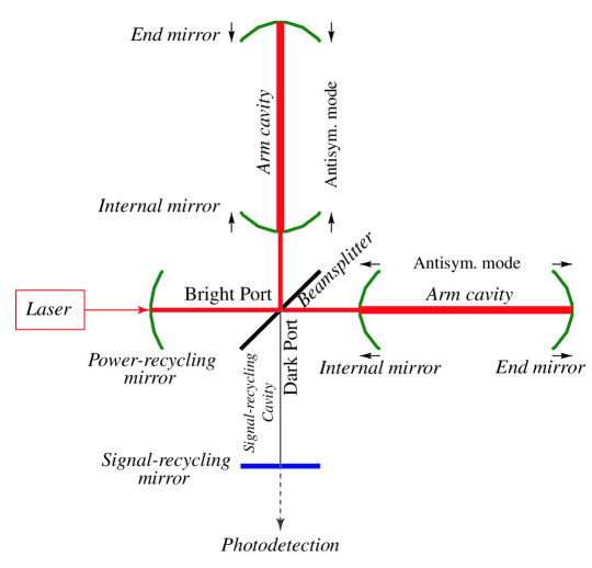
FIG. 1.: Schematic diagram of a signal recycled interferometer such as LIGO-II. The antisymmetric mode of motion of the four arm-cavity mirrors (marked by arrows) is monitored by laser interferometry. A signal-recycling mirror is used to feed the signal light back into the arm cavities, while a power-recycling mirror is introduced to feed back into the arm cavities the unused laser light coming out the bright port.

The SR mirror (see Fig. 1) sends the signal coming out the dark port back into the arm cavities; in this sense it recycles the signal. The optical system composed of the SR cavity and the arm cavities forms a composite resonant cavity, whose eigenfrequencies and quality factors can be controlled by the position and reflectivity of the SR mirror. Near its eigenfrequencies (resonances), the device can gain sensitivity. In fact, the initial motivation for introducing the SR cavity was based on the idea of using this feature to reshape the noise curves, enabling the interferometer to work either in broadband or in narrowband configurations, and improving in this way the observation of specific GW astrophysical sources [2]. Historically, the first idea for a narrowband configuration, so-called synchronous or resonant recycling, was due to Drever [4] and was subsequently analyzed by Vinet et al. [5]. It used a different optical topology from Fig. 1. The original idea for the optical topology of Fig. 1 was due to Meers [6], who proposed its use for dual recycling – a scheme which by recycling the signal light increases the storage time of the signal inside the interferometer and lowers the shot noise. Later, Mizuno et al. [7, 8, 9] proposed another scheme called Resonant Sideband Extraction (RSE), which also uses the optical topology of Fig. 1 but adjusts the SR mirror so that the storage time of the signal inside the interferometer decreases while the observation bandwidth increases. In general, by choosing appropriate detunings of the SR cavity, the optical configuration can be in either of the two regimes, or in between. These schemes have been experimentally tested by Freise et al. [10] with the 30 m laser interferometer in Garching (Germany), and by Mason [11] on a table-top experiment at Caltech (USA).

All the above mentioned theoretical analyses and experiments of SR interferometers [4, 5, 6, 7, 8, 9, 10, 11] refer to configurations with low laser power, for which the radiation pressure on the arm-cavity mirrors is negligible and the noise spectra are dominated by shot noise. However, when the laser power is increased, the shot noise decreases while the effect of radiation-pressure fluctuation increases. LIGO-II has been planned to work at a laser power for which the two effects are comparable in the observation band $10$–$200$ Hz [3]. Therefore, to correctly describe the quantum optical noise in LIGO-II, the results so far obtained in the literature [4, 5, 6, 7, 8, 9, 10, 11] must be complemented by a thorough investigation of the influence of the radiation-pressure force on the mirror motion.

Until recently the LIGO-II noise curves were computed using a semiclassical approach [3], which, although capable of estimating the shot noise, is unable to take into account correctly the effects of radiation-pressure fluctuations. Very recently, building on earlier work of Kimble, Levin, Matsko, Thorne and Vyatchanin (KLMTV for short) [12], which describes the initial optical configuration of LIGO/TAMA/VIRGO interferometers (so-called conventional interferometers) within a full quantum-mechanical approach, we investigated the SR optical configuration (Fig. 1) [13, 14]. Our analysis revealed important new properties of SR interferometers, including: (i) the presence of correlations between shot noise and radiation-pressure noise, (ii) the possibility of beating the standard quantum limit (SQL) by a modest amount, roughly a factor of two over a bandwidth of $\Delta f\!\sim\!f$ and (iii) the presence of instabilities in the optical-mechanical system formed by the optical fields and the arm-cavity mirrors. We also noticed [14] that the way the SQL is beaten in SR interferometer is quite different from standard quantum-nondemolition (QND) techniques [17] based on building up correlations between shot noise and radiation-pressure noise by (i) injecting squeezed vacuum into an interferometer’s dark port [18] and/or (ii) introducing two kilometer-long filter cavities into the interferometer’s output port [19, 12] and applying homodyne detection on the filtered light. Indeed, our analyses suggest that the improvement in the noise curves comes largely from the resonant features introduced by the SR cavity: whereas the amplitude of the classical output signal is amplified near the resonances, the output quantum fluctuation is not strongly affected by them. This way of using resonances to beat the SQL was first proposed by Braginsky, Khalili and colleagues in their scheme of “optical bar” GW detectors [20], where similarly the test mass is effectively an oscillator whose restoring force is provided by in-cavity optical fields. For an “optical bar” the free-mass SQL is irrelevant and we can beat the free-mass SQL using classical techniques of position monitoring [20].

In Ref. [14] our analysis was mainly focused on determining the input–output relations for the electromagnetic quadrature fields in a SR interferometer, and evaluating the corresponding noise spectral density. The resonant features of the whole device were discussed only briefly. In the present paper we give a detailed description of the dynamics of the system formed by the optical fields and the mirrors, we discuss the origin of the resonances and their possible instabilities, and we analyze the suppression of the instabilities by an appropriate control system. In our analysis we have found the Braginsky-Khalili formalism for linear quantum measurements [21] very powerful and intuitive, and we use it throughout this paper.

This paper is divided into two parts: the formalism and its application. In Sec. II we introduce the force-susceptibility formalism and discuss some general features of linear quantum-measurement devices. In particular, after briefly commenting in Sec. II A on general quantum-measurement systems, we derive in Sec. II B the equations of motion for linear quantum-measurement devices; in Sec. II C we write down a set of conditions on the susceptibilities of linear quantum-measurement systems; in Sec. II D we use these conditions to construct an effective description of a quantum-measurement process which allows us to identify in a straightforward way the shot noise and the radiation-pressure noise. In the subsequent sections we apply the formalism developed in Sec. II to SR interferometers. In Sec. III we show that SR interferometers can be described by the force-susceptibility formalism and we derive their equations of motion, pointing out the existence of a “ponderomotive rigidity”. In Sec. IV we discuss in detail the oscillatory behavior of the system induced by the ponderomotive rigidity, its resonances and instabilities. In Sec. V we describe the suppression of the instability by a feed-back control system which does not compromise the sensitivity. Finally, Sec. VI summarizes our main conclusions. As a foundation for our linear analysis of SR interferometers we summarize in Appendix A some general properties of linear quantum-mechanical systems.

II Quantum-measurement systems

A General conditions defining a measurement system

Following Braginsky and Khalili [21], we define a measurement process as a transformation from some original classical observable which is unknown, e.g., the gravitational-wave amplitude, into another classical observable which is known, e.g., the data stored in the computer. Generally, the system which implements this process is composed of a probe ${\cal P}$, which is directly coupled to the classical observable to be measured (for interferometers this is the antisymmetric mode of motion of the four arm-cavity mirrors, see Sec. III A), and the detector ${\cal D}$, which couples to the probe and produces the output observable (for interferometers this is the optical system and the photodetector). A measurement system is drawn schematically in Fig. 2. Because the probe and the detector are quantum mechanical systems, the overall device is called a quantum-measurement device. The output observable $\widehat{Z}={\cal S}+\widehat{\cal Q}$ contains a classical part ${\cal S}$, which depends on the classical observable $G$ to be measured, and some quantum noise $\widehat{\cal Q}$ due to the probe, the detector and their mutual interaction.

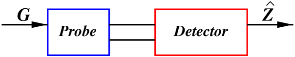
FIG. 2.: Schematic diagram of a measurement device. $G$ is the classical observable acting on the probe that we want to measure, and $\widehat{Z}$ is the detector’s observable which describes the output of the measurement system.

According to the statistical interpretation of Quantum Mechanics [23], the output of a quantum-measurement process at different times should be simultaneously measurable. One sufficient condition for simultaneous measurability is that the Heisenberg operators of the output observable, $\widehat{Z}(t)$, satisfy

$$\left[\widehat{Z}(t_{1}),\widehat{Z}(t_{2})\right]=0\quad\forall t_{1},\,t_{2}\,.$$ (1)

Henceforth, we shall regard Eq. (1) as the condition of simultaneous measurability. Although the condition (1) was originally introduced by Braginsky et al. [17, 21] as the definition of quantum-nondemolition (QND) observables (see also Refs. [24, 25, 26]), we introduce and use it for different purposes, as will become clear in the following. If the condition (1) is satisfied, then any sample of data $\left\{\widehat{Z}(t_{1}),\widehat{Z}(t_{2}),\ldots,\widehat{Z}(t_{n})\right\}$ can be stored directly as bits of classical data in a classical storage medium, and any noise from subsequent processing of the signal can be made arbitrarily small, i.e. all quantum noises are included in the quantum fluctuations of $\widehat{Z}(t)$. We want to discuss the simultaneous measurability condition (1) more deeply by pointing out the following relation, which was also in part discussed by Unruh [24] and Caves, Thorne, Drever, Sandberg and Zimmermann in Sec. IV of Ref. [25], and reviewed subsequently in Ref. [26], although from a different point of view.

Simultaneous-Measurability – Zero-Response Relation: For a Quantum Measurement Device (QMD), the simultaneous measurability condition for the output $\widehat{Z}(t)$, i.e. $[\widehat{Z}(t_{1}),\widehat{Z}(t_{2})]=0\quad\forall t_{1},\,t_{2}$, is equivalent to requiring that if the device is coupled to an external system via an interaction Hamiltonian of the form $V(\widehat{Z},\widehat{\cal E})$ where $V$ is an arbitrary function and $\widehat{\cal E}$ belongs to the external system, then the back action on the QMD does not alter the evolution of the output observable $\widehat{Z}$.

Proof of necessity. Let us suppose that our QMD with output $\widehat{Z}$ evolves under a Hamiltonian $\widehat{H}_{\rm QMD}$, and that $[\widehat{Z}(t),\widehat{Z}(t^{\prime})]=0$ for all $t,t^{\prime}$. Now let us couple it to an arbitrary external system with Hamiltonian $\widehat{H}_{\rm EXT}$ via a generic interaction term $V(\widehat{Z},\widehat{\cal E})$ as specified above, where $\widehat{\cal E}$ is an observable of the external system. The total Hamiltonian is

$$\widehat{H}=\left(\widehat{H}_{\rm QMD}+\widehat{H}_{\rm EXT}\right)+V(\widehat{Z},\widehat{\cal E})\,.$$ (2)

If we treat the two terms in the bracket as the zeroth-order Hamiltonian and the interaction Hamiltonian $V(\widehat{Z},\widehat{\cal E})$ as a perturbation, by applying the results derived in the Appendix [see Eq. (A14)] we can write the Heisenberg operator of the output variable $\widehat{Z}$ as,

$$\widehat{Z}_{\rm pert}(t)=\widehat{Z}(t)+\frac{i}{\hbar}\int_{-\infty}^{t}dt_{1}\left[V(\widehat{Z}(t_{1}),\widehat{\cal E}(t_{1})),\widehat{Z}(t)\right]+$$ (3)

$$\left(\frac{i}{\hbar}\right)^{2}\int_{-\infty}^{t}dt_{1}\int_{-\infty}^{t_{1}}dt_{2}\left[V(\widehat{Z}(t_{2}),\widehat{\cal E}(t_{2})),\left[V(\widehat{Z}(t_{1}),\widehat{\cal E}(t_{1})),\widehat{Z}(t)\right]\right]+\cdots\,,$$ (4)

with higher order terms of the form [see Eq. (A14)]:

$$\left[V(\widehat{Z}(t_{n}),\widehat{\cal E}(t_{n})),\left[\cdots,\left[V(\widehat{Z}(t_{2}),\widehat{\cal E}(t_{2})),\left[V(\widehat{Z}(t_{1}),\widehat{\cal E}(t_{1})),\widehat{Z}(t)\right]\right]\cdots\right]\right]\,.$$ (5)

Here $\widehat{Z}(t)$ and $\widehat{\cal E}(t)$ evolve under the Hamiltonians $\widehat{H}_{\rm QMD}$ and $\widehat{H}_{\rm EXT}$, respectively. Because they belong to two different Hilbert spaces we have $[\widehat{Z}(t),\widehat{\cal E}(t^{\prime})]=0$ for all $t,t^{\prime}$. By assumption, we also have $[\widehat{Z}(t_{1}),\widehat{Z}(t_{2})]=0\quad\forall t_{1},\,t_{2}$. Using these two facts, we obtain $[V(\widehat{Z}(t_{1}),\widehat{\cal E}(t_{1})),\widehat{Z}(t_{2})]=0\quad\forall t_{1},\,t_{2}$, and then using Eq. (4) we derive $\widehat{Z}_{\rm pert}(t)=\widehat{Z}(t)$. This means that the evolution of $\widehat{Z}$ is not affected by the kind of external coupling we introduced.

Proof of sufficiency. Let us suppose the evolution of $\widehat{Z}$ is not affected by any external system of the form specified above. Then, in particular, it must be true for the simple interaction Hamiltonian $V(\widehat{Z},\widehat{\cal E})=-\alpha\widehat{Z}\,{\cal E}$, where $\alpha$ is some coupling constant which can vary continuously, e.g., in the interval $(0,1]$, and we choose a classical external coupling ${\cal E}$. In this particular case Eq. (4) becomes

$$\widehat{Z}_{\rm pert}(t)=\widehat{Z}(t)-\alpha\,\frac{i}{\hbar}\,\int_{-\infty}^{t}dt_{1}\left[\widehat{Z}(t_{1}),\widehat{Z}(t)\right]\,{\cal E}(t_{1})+O(\alpha^{2})\,,$$ (6)

with higher order terms of the form: $\alpha^{n}\,[\widehat{Z}(t_{n}),[\cdots,[\widehat{Z}(t_{2}),[\widehat{Z}(t_{1}),\widehat{Z}(t)]]\cdots]]$. By assumption the LHS of Eq. (6) does not change when we vary $\alpha$. The RHS of Eq. (6) is a power series in $\alpha$, and using the uniqueness of the Taylor expansion, we deduce that all the terms beyond the zeroth order should vanish separately. In particular, the first-order term should vanish and we conclude that $[\widehat{Z}(t),\widehat{Z}(t^{\prime})]=0$ for all $t,t^{\prime}$. $\Box$

Let us comment on two interesting aspects of the Simultaneous-Measurability – Zero-Response Relation given above.

• This relation links the abstract quantum mechanical idea of simultaneous measurability to the classical dynamics of the measurement device, yielding a simple criterion for the quantum-classical transition: the observable which corresponds to the classical output variable should have no response to external perturbations directly coupled to it. We shall use this criterion in our analysis of linear systems in Sec. II C.

• This relation is also interesting conceptually. In practice, the result of every measurement is read out by coupling the measurement device to another system, and the boundary between the “measurement” (still part of the QMD) and the “data analysis” (external to the QMD) occurs at a “stage” at which no possible direct coupling to the output observable could change the evolution of the output observable itself. Otherwise at that stage the “external coupling” should still be considered as part of the measurement device.

Before ending this section, let us compare the point of view followed in this section to the one pursued in previous QND analyses [24, 25, 26], especially Sec. IV of Ref. [25]. The authors of Refs. [25, 26] followed two steps in their discussion. First, they searched for a class of observables $\widehat{A}(t)$ of a quantum-mechanical system that can be monitored without adding fundamental noise, deducing a condition for $\widehat{A}(t)$ that coincides with Eq. (1). They called such observables QND observables. Secondly, they found appropriate interaction Hamiltonians describing the coupling between $\widehat{A}(t)$ and a measuring apparatus that do not disturb the evolution of $\widehat{A}(t)$ during the measurement process. However, in Refs. [25, 26] there is no clear distinction between what we call the detector and the external measurement system; these two systems are referred to together as the measuring apparatus. Thus, the observable $\widehat{A}(t)$ does not necessarily coincide with the output $\widehat{Z}(t)$ of our probe-detector system, and for this reason we prefer not to call it a QND observable in the sense of Refs. [24, 25, 26].

As a final remark, we note that whereas in Refs. [25, 26] the measuring apparatus and the interaction Hamiltonian are indispensable parts of a measurement process, in this paper, by distinguishing the detector from the external system, we use the latter only as part of a gedanken experiment, by which we clarify the relation between simultaneous measurability and the response to external couplings, which will lead to useful properties of linear quantum-measurement devices in Sec. II C.

B Equations of motion of a linear quantum-measurement system: The force-susceptibility formalism

Starting in this section we shall focus on linear measurement systems. We shall see in Sec. III that GW interferometers belong to this class of devices. Our analysis has been inspired by the formalism of linear quantum-measurement theory introduced by Braginsky and Khalili (Chaps. V, VI and VII of Ref. [21]) and is based on the force-susceptibility description of linearly coupled systems under linearly applied classical forces (see, e.g., Sec. 6.4 of Ref. [21]).

In a linear measurement process, the device acts linearly and is linearly coupled to the classical observable to be measured (see the Appendix for a precise definition of linear systems). We suppose that the device can be artificially divided into two linearly coupled, but otherwise independent subsystems: the probe, which is subject to the external classical force we want to measure, and the detector, which yields a classical output. More specifically, in our Hamiltonian system the probe is coupled to the external classical force $G$ by $-\widehat{y}\,G$, where $\widehat{y}$ is some linear observable of the probe, while the probe and the detector are coupled by a term $-\widehat{x}\,\widehat{F}$, where $\widehat{x}$ is a generalized (linear) displacement of the probe, and $\widehat{F}$ is a linear observable of the detector which describes its back-action force on the probe. In general, the observable $\widehat{x}$ to which the external force is coupled and the observable $\widehat{y}$ that the detector directly measures might not be the same. However, in our idealized model of GW interferometers (Sec. III below), $\widehat{x}$ and $\widehat{y}$ are actually the same observable, namely the generalized coordinate of the antisymmetric mode of motion of the four arm-cavity mirrors (see Fig. 1 and Sec. III A), and $\widehat{F}$ is the radiation-pressure force acting on this mode. Henceforth, we shall impose $\widehat{y}\equiv\widehat{x}$. Finally, we denote by $\widehat{Z}$ the linear observable of the detector which describes the output of the entire device. A sketchy representation of the measurement device is drawn in Fig. 3. The linear observables $\widehat{x}$ describing the probe ${\cal P}$ and $\widehat{Z}$, $\widehat{F}$ describing the detector ${\cal D}$ belong to two different Hilbert spaces $\cal{H}_{\cal P}$ and $\cal{H}_{\cal D}$, respectively, and the Hilbert space of the combined system is $\cal{H}_{\cal P}\otimes\cal{H}_{\cal D}$. The Hamiltonian is given by

$$\widehat{H}=\left[\left(\widehat{H}_{\cal P}-\widehat{x}\,G\right)+\widehat{H}_{\cal D}\right]-\widehat{x}\,\widehat{F}\,.$$ (7)

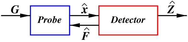
FIG. 3.: Schematic diagram of a linear measurement system. $G$ is the external classical force acting on the probe that we want to measure, $\widehat{x}$ is the linear observable of the probe, $\widehat{F}$ is the linear observable of the detector which describes the back-action force on the probe, and $\widehat{Z}$ is the linear observable of the detector which describes the output of the overall measurement system.

We shall now derive the equations of motion of the system composed of the linear observables $\widehat{x}$, $\widehat{Z}$ and $\widehat{F}$. As a first step in our calculation, we regard the Hamiltonians $\widehat{H}_{\cal P}-\widehat{x}\,G$ and $\widehat{H}_{\cal D}$ as zeroth order Hamiltonians for the subsystems ${\cal P}$ and ${\cal D}$, respectively, and we treat $-\widehat{x}\,\widehat{F}$ as a linear coupling between ${\cal P}$ and ${\cal D}$. Working in the Heisenberg picture, we obtain the following equations [see Theorem 4 of the Appendix and Eqs. (A17), (A18)]:

$$\widehat{Z}^{(1)}(t) = \widehat{Z}^{(0)}(t)+\frac{i}{\hbar}\int_{-\infty}^{t}dt^{\prime}\,C_{Z^{(0)}F^{(0)}}(t,t^{\prime})\,\widehat{x}^{(1)}(t^{\prime})\,,$$ (8)

$$\widehat{F}^{(1)}(t) = \widehat{F}^{(0)}(t)+\frac{i}{\hbar}\int_{-\infty}^{t}dt^{\prime}\,C_{F^{(0)}F^{(0)}}(t,t^{\prime})\,\widehat{x}^{(1)}(t^{\prime})\,,$$ (9)

$$\widehat{x}^{(1)}(t) = \widehat{x}^{(G)}(t)+\frac{i}{\hbar}\int_{-\infty}^{t}dt^{\prime}\,C_{x^{(G)}x^{(G)}}(t,t^{\prime})\,\widehat{F}^{(1)}(t^{\prime})\,.$$ (10)

Here $C_{AB}(t,t^{\prime})$ is a complex number (C-number), called the (time-domain) susceptibility, and is defined by Eq. (A16) of the Appendix, i.e.

$$C_{AB}(t,t^{\prime})\equiv\left[\widehat{A}(t),\,\widehat{B}(t^{\prime})\right]\,.$$ (11)

[Henceforth, we shall often use the expressions different-time commutator and time-domain susceptibility interchangeably.] The superscript ${(1)}$ in Eqs. (8)–(10) denotes time evolution under the total Hamiltonian $\widehat{H}$ [Eq. (7)], the superscript ${(0)}$ on $\widehat{F}(t)$ and $\widehat{Z}(t)$ denotes time evolution under the free Hamiltonian of the detector $\widehat{H}_{\cal D}$, while the superscript ${(G)}$ on $\widehat{x}(t)$ refers to the time evolution under the Hamiltonian $\widehat{H}_{\cal P}-\widehat{x}\,G$, which describes the probe under the sole influence of $G(t)$.

As a second step, we want to relate $\widehat{x}^{(G)}(t)$ to $\widehat{x}^{(0)}(t)$, which evolves under the free probe Hamiltonian $\widehat{H}_{\cal P}$. Using Theorem 3 in the Appendix and Eqs. (A15), (A16), we deduce

$$\widehat{x}^{(G)}(t)=\widehat{x}^{(0)}(t)+\frac{i}{\hbar}\int_{-\infty}^{t}dt^{\prime}\,C_{x^{(0)}x^{(0)}}(t,t^{\prime})\,G(t^{\prime})\,.$$ (12)

Noticing from Eq. (12) that $\widehat{x}^{(G)}$ differs from $\widehat{x}^{(0)}$ by a time dependent C-number, we get $C_{x^{(G)}x^{(G)}}(t,t^{\prime})=C_{x^{(0)}x^{(0)}}(t,t^{\prime})$. Using this fact and inserting Eq. (12) into Eq. (10), we can relate the Heisenberg operators evolving under the full Hamiltonian $\widehat{H}$ to those evolving under the free Hamiltonians of the probe and the detector $\widehat{H}_{\cal P}$ and $\widehat{H}_{\cal D}$ separately:

$$\widehat{Z}^{(1)}(t) = \widehat{Z}^{(0)}(t)+\frac{i}{\hbar}\int_{-\infty}^{t}dt^{\prime}\,C_{Z^{(0)}F^{(0)}}(t,t^{\prime})\,\widehat{x}^{(1)}(t^{\prime})\,,$$ (13)

$$\widehat{F}^{(1)}(t) = \widehat{F}^{(0)}(t)+\frac{i}{\hbar}\int_{-\infty}^{t}dt^{\prime}\,C_{F^{(0)}F^{(0)}}(t,t^{\prime})\,\widehat{x}^{(1)}(t^{\prime})\,,$$ (14)

$$\widehat{x}^{(1)}(t) = \widehat{x}^{(0)}(t)+\frac{i}{\hbar}\int_{-\infty}^{t}dt^{\prime}\,C_{x^{(0)}x^{(0)}}(t,t^{\prime})\,[G(t^{\prime})+\widehat{F}^{(1)}(t^{\prime})]\,.$$ (15)

A quantity of special interest for us is the displacement induced on a free probe (without any influence of the detector) by $G(t)$, namely the second term on the RHS of Eq. (12). For a GW interferometer this displacement is $L\,h(t)$, where $L$ is the arm-cavity length and $h(t)$ is the differential strain induced by the gravitational wave on the free arm-cavity mirrors (the difference in strain between the two arms). In our notation we denote this quantity by

$$L\,h(t)=\frac{i}{\hbar}\int_{-\infty}^{t}dt^{\prime}\,C_{x^{(0)}x^{(0)}}(t,t^{\prime})\,G(t^{\prime})\,,$$ (16)

and for a GW interferometer $G(t)=(m/4)\,L\,\ddot{h}(t)$, where $m/4$ is the reduced mass of the antisymmetric mode of motion of the four arm-cavity mirrors (see Secs. III A and III B). [Note that each mirror has mass $m$.]

Henceforth, we shall assume that both the probe and the detector have time independent Hamiltonians, i.e. both $\widehat{H}_{\cal D}$ and $\widehat{H}_{\cal P}$ are time independent. In this case, as shown in the Appendix, the susceptibilities that appear in Eqs. (13)–(15) depend only on $t-t^{\prime}$. By transforming them into the Fourier domain, denoting by $h(\Omega)$ the Fourier transform of $h(t)$ and introducing the Fourier-domain susceptibility

$$R_{AB}(\Omega)\equiv\frac{i}{\hbar}\int_{0}^{+\infty}d\tau\,e^{i\Omega\tau}\,C_{AB}(0,-\tau)\,,$$ (17)

we derive

$$\widehat{Z}^{(1)}(\Omega) = \widehat{Z}^{(0)}(\Omega)+R_{ZF}(\Omega)\,\widehat{x}^{(1)}(\Omega)\,,$$ (18)

$$\widehat{F}^{(1)}(\Omega) = \widehat{F}^{(0)}(\Omega)+R_{FF}(\Omega)\,\widehat{x}^{(1)}(\Omega)\,,$$ (19)

$$\widehat{x}^{(1)}(\Omega) = \widehat{x}^{(0)}(\Omega)+L\,h(\Omega)+R_{xx}(\Omega)\,\widehat{F}^{(1)}(\Omega)\,.$$ (20)

Here and below, to simplify the notation we denote $R_{ZF}\equiv R_{Z^{(0)}F^{(0)}}$, $R_{FF}\equiv R_{F^{(0)}F^{(0)}}$, $R_{xx}\equiv R_{x^{(0)}x^{(0)}}$. By solving Eqs. (18)–(20) for the full-evolution operators in terms of the free-evolution ones, we finally get:

$$\widehat{x}^{(1)}(\Omega) = \frac{1}{1-R_{xx}(\Omega)\,R_{FF}(\Omega)}\,\left[\widehat{x}^{(0)}(\Omega)+L\,h(\Omega)+R_{xx}(\Omega)\,\widehat{F}^{(0)}(\Omega)\right]\,,$$ (21)

$$\widehat{F}^{(1)}(\Omega) = \frac{1}{1-R_{xx}(\Omega)\,R_{FF}(\Omega)}\,\left[\widehat{F}^{(0)}(\Omega)+R_{FF}(\Omega)\,\left(\widehat{x}^{(0)}(\Omega)+L\,h(\Omega)\right)\right]\,,$$ (22)

$$\widehat{Z}^{(1)}(\Omega) = \widehat{Z}^{(0)}(\Omega)+\frac{R_{ZF}(\Omega)}{1-R_{xx}(\Omega)\,R_{FF}(\Omega)}\,\left[\widehat{x}^{(0)}(\Omega)+L\,h(\Omega)+R_{xx}(\Omega)\,\widehat{F}^{(0)}(\Omega)\right]\,.$$ (23)

Let us point out that if the kernel relating the full-evolution operators to the free-evolution ones, i.e.  $1/(1-R_{xx}\,R_{FF})$, contains poles both in the lower and in the upper complex plane [with our definition of Fourier transform given by Eq. (A19)], then by applying the standard inverse Fourier transform to Eqs. (21)–(23), we get that $\widehat{x}^{(1)}(t)$, $\widehat{F}^{(1)}(t)$ and $\widehat{Z}^{(1)}(t)$ depend on the gravitational-wave field and the free-evolution operators $\widehat{x}^{(0)}(t)$, $\widehat{F}^{(0)}(t)$ and $\widehat{Z}^{(0)}(t)$ both in the past and in the future. However, these are not the correct solutions for the real motion. This situation is a very common one in physics and engineering (it occurs for example in the theory of linear electronic networks [22] and the theory of plasma waves [27]), and the cure for it is well known: in order to obtain the (correct) full-evolution operators $\widehat{x}^{(1)}(t)$, $\widehat{F}^{(1)}(t)$ and $\widehat{Z}^{(1)}(t)$ that only depend on the past, we have to alter the integration contour in the inverse-Fourier transform, going above all the poles in the complex plane. [In the language of plasma physics we have to use the Landau contours.] This procedure, which can be justified rigorously using Laplace transforms [28], makes $\widehat{x}^{(1)}(t)$, $\widehat{F}^{(1)}(t)$ and $\widehat{Z}^{(1)}(t)$ for many systems (including LIGO-II interferometers) infinitely sensitive to driving forces in the infinitely distant past. The reason is simple and well known in other contexts: such quantum-measurement systems possess instabilities, which can be deduced from the homogeneous solutions of Eqs. (21)–(23), whose eigenfrequencies are given by the equation $1-R_{xx}(\Omega)\,R_{FF}(\Omega)=0$. The zeros of the equation $1-R_{xx}(\Omega)\,R_{FF}(\Omega)=0$ are generically complex and for unstable systems they have positive imaginary parts, corresponding to homogeneous solutions that grow exponentially toward the future.

C Conditions defining a linear measurement system in terms of susceptibilities

As we pointed out in Sec. II A, in order to be identified as the output of the measurement system, the observable $\widehat{Z}$ should satisfy $[\widehat{Z}(t_{1}),\widehat{Z}(t_{2})]=0,\;\forall\,t_{1},\,t_{2}$, i.e. the condition of simultaneous measurability. In that section, we have also proved the equivalence between this condition and the condition that any external coupling to the measurement system through $\widehat{Z}$ should not change the evolution of $\widehat{Z}$ itself. In the following we shall take advantage of this equivalence: By imagining that we couple the linear measurement system to some external system through $\widehat{Z}$ and by looking at (possible) changes in $\widehat{Z}$’s evolution, we shall obtain a set of conditions for the susceptibilities involving $\widehat{Z}$.

Let us first restrict ourselves to the simplest possible external coupling, $\widehat{V}=-\widehat{Z}\,{\cal E}$, where ${\cal E}$ is a classical external force. The total Hamiltonian (7) becomes

$$\widehat{H}=\left[\left(\widehat{H}_{\cal P}-\widehat{x}\,G\right)+\widehat{H}_{\cal D}\right]-\widehat{x}\,\widehat{F}-\widehat{Z}\,{\cal E}=\left[\left(\widehat{H}_{\cal P}-\widehat{x}\,G\right)+\left(\widehat{H}_{\cal D}-\widehat{Z}\,{\cal E}\right)\right]-\widehat{x}\,\widehat{F}\,.$$ (24)

To derive the equations of motion for the Hamiltonian (24) we apply the procedure used in Sec. II B to deduce the equations of motion for the Hamiltonian (7). First, we consider $(\widehat{H}_{\cal P}-\widehat{x}\,G)$ and $(\widehat{H}_{\cal D}-\widehat{Z}\,{\cal E})$ as zeroth order Hamiltonians and relate the operators $\widehat{Z}^{(1)}_{\rm pert}$, $\widehat{F}^{(1)}_{\rm pert}$ and $\widehat{x}^{(1)}_{\rm pert}$, which evolve under the full Hamiltonian (24), to the operator $\widehat{x}^{(G)}$, which evolves under the Hamiltonian $(\widehat{H}_{\cal P}-\widehat{x}\,G)$, and the operators $\widehat{Z}^{({\cal E})}$ and $\widehat{F}^{({\cal E})}$, evolving under the Hamiltonian $(\widehat{H}_{\cal D}-\widehat{Z}\,{\cal E})$,

$$\widehat{Z}^{(1)}_{\rm pert}(t) = \widehat{Z}^{({\cal E})}_{\rm pert}(t)+\frac{i}{\hbar}\int_{-\infty}^{t}dt^{\prime}\,C_{Z^{({\cal E})}F^{({\cal E})}}(t,t^{\prime})\,\widehat{x}^{(1)}_{\rm pert}(t^{\prime})\,,$$ (25)

$$\widehat{F}^{(1)}_{\rm pert}(t) = \widehat{F}^{({\cal E})}_{\rm pert}(t)+\frac{i}{\hbar}\int_{-\infty}^{t}dt^{\prime}\,C_{F^{({\cal E})}F^{({\cal E})}}(t,t^{\prime})\,\widehat{x}^{(1)}_{\rm pert}(t^{\prime})\,,$$ (26)

$$\widehat{x}^{(1)}_{\rm pert}(t) = \widehat{x}^{(G)}(t)+\frac{i}{\hbar}\int_{-\infty}^{t}dt^{\prime}\,C_{x^{(G)}x^{(G)}}(t,t^{\prime})\,\widehat{F}^{(1)}_{\rm pert}(t^{\prime})\,.$$ (27)

Second, we relate the operators $\widehat{x}^{(G)}$, $\widehat{Z}^{({\cal E})}$ and $\widehat{F}^{({\cal E})}$ to the operators $\widehat{x}^{(0)}$, $\widehat{Z}^{(0)}$ and $\widehat{F}^{(0)}$ which evolve under $\widehat{H}_{\cal P}$ and $\widehat{H}_{\cal D}$:

$$\widehat{Z}^{({\cal E})}_{\rm pert}(t) = \widehat{Z}^{(0)}(t)+\frac{i}{\hbar}\int_{-\infty}^{t}dt^{\prime}\,C_{Z^{(0)}Z^{(0)}}(t,t^{\prime})\,{\cal E}(t^{\prime})\,,$$ (28)

$$\widehat{F}^{({\cal E})}_{\rm pert}(t) = \widehat{F}^{(0)}(t)+\frac{i}{\hbar}\int_{-\infty}^{t}dt^{\prime}\,C_{F^{(0)}Z^{(0)}}(t,t^{\prime})\,{\cal E}(t^{\prime})\,,$$ (29)

$$\widehat{x}^{(G)}(t) = \widehat{x}^{(0)}(t)+\frac{i}{\hbar}\int_{-\infty}^{t}dt^{\prime}\,C_{x^{(0)}x^{(0)}}(t,t^{\prime})\,G(t^{\prime})\,.$$ (30)

Noticing that $\widehat{Z}^{({\cal E})}_{\rm pert}$, $\widehat{F}^{({\cal E})}_{\rm pert}$ and $\widehat{x}^{(G)}$ differ from $\widehat{Z}^{(0)}$, $\widehat{F}^{(0)}$ and $\widehat{x}^{(0)}$ only by time dependent C-numbers, we obtain the following relations: $C_{Z^{({\cal E})}F^{({\cal E})}}(t,t^{\prime})=C_{Z^{(0)}F^{(0)}}(t,t^{\prime})$, $C_{F^{({\cal E})}F^{({\cal E})}}(t,t^{\prime})=C_{F^{(0)}F^{(0)}}(t,t^{\prime})$ and $C_{x^{(G)}x^{(G)}}(t,t^{\prime})=C_{x^{(0)}x^{(0)}}(t,t^{\prime})$. Then, by inserting Eqs. (28)–(30) into Eqs. (25)–(27), we deduce the equations of motion of $\widehat{Z}$, $\widehat{F}$ and $\widehat{x}$ under the Hamiltonian (24):

$$\widehat{Z}^{(1)}_{\rm pert}(t) = \widehat{Z}^{(0)}(t)+\frac{i}{\hbar}\int_{-\infty}^{t}dt^{\prime}\,\left[C_{Z^{(0)}Z^{(0)}}(t,t^{\prime})\,{\cal E}(t^{\prime})+C_{Z^{(0)}F^{(0)}}(t,t^{\prime})\,\widehat{x}^{(1)}_{\rm pert}(t^{\prime})\right]\,,$$ (31)

$$\widehat{F}^{(1)}_{\rm pert}(t) = \widehat{F}^{(0)}(t)+\frac{i}{\hbar}\int_{-\infty}^{t}dt^{\prime}\,\left[C_{F^{(0)}Z^{(0)}}(t,t^{\prime})\,{\cal E}(t^{\prime})+C_{F^{(0)}F^{(0)}}(t,t^{\prime})\,\widehat{x}^{(1)}_{\rm pert}(t^{\prime})\right]\,,$$ (32)

$$\widehat{x}^{(1)}_{\rm pert}(t) = \widehat{x}^{(0)}(t)+\frac{i}{\hbar}\int_{-\infty}^{t}dt^{\prime}\,C_{x^{(0)}x^{(0)}}(t,t^{\prime})\,\left[G(t^{\prime})+\widehat{F}^{(1)}_{\rm pert}(t^{\prime})\right]\,.$$ (33)

From Eqs. (31)–(33) we infer that there are two ways the external force ${\cal E}$ can influence the evolution of $\widehat{Z}^{(1)}_{\rm pert}$: (i) ${\cal E}$ can affect $\widehat{Z}^{(1)}_{\rm pert}$ directly, through the first term in the bracket of Eq. (31), unless $C_{Z^{(0)}Z^{(0)}}(t,t^{\prime})=0$ for all $t>t^{\prime}$ (and thus for all pairs of $t$ and $t^{\prime}$); and (ii) ${\cal E}$ can influence the evolution of $\widehat{Z}^{(1)}_{\rm pert}$ indirectly, affecting the evolution of $\widehat{F}^{(1)}_{\rm pert}$ [first term in the bracket of Eq. (32)], and through it the evolution of $\widehat{x}^{(1)}_{\rm pert}$ and $\widehat{Z}^{(1)}_{\rm pert}$ [second terms in the brackets of Eqs. (33), (31)], unless $C_{F^{(0)}Z^{(0)}}(t,t^{\prime})=0$ for all $t>t^{\prime}$.

Now we are ready to deduce the conditions that must be satisfied in order that the evolution of $\widehat{Z}$ not be changed by the external coupling ${\cal E}$. In principle the two ways ${\cal E}$ affects the evolution of $\widehat{Z}$ may cancel each other. However, noticing the fact that case (i) does not depend on the probe (only $C_{Z^{(0)}Z^{(0)}}$ matters), but case (ii) does ($C_{x^{(0)}x^{(0)}}$ also matters), we see that the cancellation will not always occur if we assume that, whatever probe the detector is coupled to, $\widehat{Z}$ always corresponds to the output of the measurement process. Thus both conditions must be satisfied: $C_{Z^{(0)}Z^{(0)}}=0$ and $C_{F^{(0)}Z^{(0)}}=0$.

This argument for both conditions can be made more clear by assigning an “effective mass” $\mu$ to the probe and consider a continuous family of probes labeled by $\mu$ (for interferometers the family of probes are the family of mirrors with different masses). The susceptibility of the coordinate $\widehat{x}$ depends on the effective mass as

$$C_{x^{(0)}x^{(0)}}\propto\frac{1}{\mu}\,,$$ (34)

which simply says that the probe’s response to external forces decreases as its effective mass increases. Because $\widehat{Z}^{(0)}$ and $\widehat{F}^{(0)}$ are operators evolving under the free Hamiltonian of the detector, they do not depend on $\mu$. Now consider two cases: First, the limiting case of $\mu\rightarrow\infty$. Then $C_{x^{(0)}x^{(0)}}\rightarrow 0$ and from Eq. (33) we get $\widehat{x}^{(1)}_{\rm pert}(t)=\widehat{x}^{(0)}(t)$. As a consequence, ${\cal E}$ affects the evolution of $\widehat{Z}^{(1)}_{\rm pert}$ only through the first term in the bracket of Eq. (31) [see case (i) above], unless $C_{Z^{(0)}Z^{(0)}}(t,t^{\prime})=0$ for all pairs of $t$ and $t^{\prime}$. Second, consider the case of finite mass $\mu$, and then conclude that ${\cal E}$ will affect the evolution of $\widehat{Z}^{(1)}_{\rm pert}$ only through the second term in the bracket of Eq. (31) [see case (ii) above], unless $C_{F^{(0)}Z^{(0)}}(t,t^{\prime})=0$ for all $t>t^{\prime}$.

In conclusion we have found that if, whatever the probe is, $\widehat{Z}$ always corresponds to the output of the linear measurement device, then the following conditions must be satisfied

$${\rm LQM}:\left\{\begin{array}[]{rllll}C_{Z^{(0)}Z^{(0)}}(t,t^{\prime})&\equiv[\widehat{Z}^{(0)}(t),\widehat{Z}^{(0)}(t^{\prime})]&=0&&\forall\,t,t^{\prime}\\ C_{F^{(0)}Z^{(0)}}(t,t^{\prime})&\equiv[\widehat{F}^{(0)}(t),\widehat{Z}^{(0)}(t^{\prime})]&=0&&\forall\,t>t^{\prime}\,.\end{array}\right.$$ (37)

In the frequency domain these conditions read

$$R_{ZZ}(\Omega)=0=R_{FZ}(\Omega)\,.$$ (38)

It is possible to show that LQM [Eqs. (37)] are also sufficient conditions for the simultaneous measurability condition (1) be satisfied independently of the probe’s nature; imagine coupling our linear measurement system to an external system with an arbitrary Hamiltonian $H_{\rm EXT}$ via a generic coupling $V(\widehat{Z},\widehat{\cal E})$, $\widehat{\cal E}$ being an external observable, and check whether the evolution of $\widehat{Z}$ is affected by this coupling. The check can be achieved by writing the total Hamiltonian as

$$\widehat{H}=\left[\left(\widehat{H}_{\cal P}-\widehat{x}\,G\right)+\left(\widehat{H}_{\cal D}-\widehat{Z}\,\widehat{\cal E}+\widehat{H}_{\rm EXT}\right)\right]-\widehat{x}\,\widehat{F}\,,$$ (39)

and re-doing all the steps followed earlier in this section. It is helpful to notice that the evolutions of $\widehat{Z}$ and $\widehat{F}$ under $\widehat{H}_{\cal D}-\widehat{Z}\widehat{\cal E}+\widehat{H}_{\rm EXT}$ are the same as those under $\widehat{H}_{\cal D}$, once the condition LQM, or Eqs. (37), is satisfied. The result, after a long calculation is that conditions (37) are sufficient to guarantee that the evolution of $\widehat{Z}$ is unaffected by the coupling. The technical details of the proof are left as an exercise for the reader.

D Effective description of measurement systems

It is common to normalize the output observable $\widehat{Z}$ to unit signal — e.g., in the case of GW interferometer, it is common to set to unity the coefficient in front of the (classical) observable $L\,h$ we want to measure so the normalized output $\widehat{Z}$ has the form:

$$\widehat{\cal O}=\widehat{\cal N}+L\,h\,,$$ (40)

where $\widehat{\cal N}$ is the so-called signal-referred quantum noise. The observable $\widehat{\cal O}$ can be easily deduced in the frequency domain by renormalizing Eq. (23),

$$\widehat{\cal O}(\Omega) = \frac{1-R_{xx}(\Omega)\,R_{FF}(\Omega)}{R_{ZF}(\Omega)}\,\widehat{Z}^{(1)}(\Omega)$$ (41)

$$= \frac{\widehat{Z}^{(0)}(\Omega)}{R_{ZF}(\Omega)}+R_{xx}(\Omega)\left[\widehat{F}^{(0)}(\Omega)-R_{FF}(\Omega)\,\frac{\widehat{Z}^{(0)}(\Omega)}{R_{ZF}(\Omega)}\right]+\widehat{x}^{(0)}(\Omega)+L\,h(\Omega)\,,$$ (42)

that is

$$\widehat{\cal O}(\Omega)=\widehat{\cal Z}(\Omega)+R_{xx}(\Omega)\,\widehat{\cal F}(\Omega)+\widehat{x}^{(0)}(\Omega)+L\,h(\Omega)\,.$$ (43)

Here we have introduced two linear observables $\widehat{\cal Z}$ and $\widehat{\cal F}$ defined in the Hilbert space ${\cal H}_{\cal D}$ of the detector,

$$\widehat{\cal Z}(\Omega)\equiv\frac{\widehat{Z}^{(0)}(\Omega)}{R_{ZF}(\Omega)}\,,\quad\quad\widehat{\cal F}(\Omega)\equiv\widehat{F}^{(0)}(\Omega)-R_{FF}(\Omega)\,\frac{\widehat{Z}^{(0)}(\Omega)}{R_{ZF}(\Omega)}\,.$$ (44)

In the time domain the output observable $\widehat{\cal O}(t)$ reads

$$\widehat{\cal O}(t)=\int_{-\infty}^{+\infty}dt^{\prime}\,K(t-t^{\prime})\,\widehat{Z}^{(1)}(t^{\prime})$$ (45)

where

$${K}(t)=\int_{-\infty}^{+\infty}\frac{1-R_{xx}(\Omega)\,R_{FF}(\Omega)}{R_{ZF}(\Omega)}\,e^{-i\,\Omega\,t}\,\frac{d\Omega}{2\pi}\,.$$ (46)

Thus

$$\widehat{\cal O}(t)=\widehat{\cal Z}(t)+\frac{i}{\hbar}\int_{-\infty}^{t}dt^{\prime}C_{x^{(0)}x^{(0)}}(t,t^{\prime})\,\widehat{\cal F}(t^{\prime})+\widehat{x}^{(0)}(t)+L\,h(t)\,.$$ (47)

Using the two properties given by Eqs. (A22) of the Appendix, and applying the conditions LQM [Eqs. (37)], we obtain the following commutation relations for the observables $\widehat{\cal Z}(t)$ and $\widehat{\cal F}(t)$ in the Fourier domain

$$\left[\widehat{\cal Z}(\Omega),\widehat{\cal Z}^{\dagger}(\Omega^{\prime})\right]=0=\left[\widehat{\cal F}(\Omega),\widehat{\cal F}^{\dagger}(\Omega^{\prime})\right]\,,\quad\quad\left[\widehat{\cal Z}(\Omega),\widehat{\cal F}^{\dagger}(\Omega^{\prime})\right]=-2\pi\,i\hbar\,\delta(\Omega-\Omega^{\prime})\,,$$ (48)

or in the time domain:

$$\left[\widehat{\cal Z}(t),\widehat{\cal Z}(t^{\prime})\right]=0=\left[\widehat{\cal F}(t),\widehat{\cal F}(t^{\prime})\right]\;\;\;\;\;\forall\,t,t^{\prime}\,,$$ (49)

$$\left[\widehat{\cal Z}(t),\widehat{\cal F}(t^{\prime})\right]=-i\hbar\,\delta(t-t^{\prime})\;\;\;\;\;\forall\,t,t^{\prime}\,.$$ (50)

It is interesting to notice that, because the observables $\widehat{\cal Z}(t)$ and $\widehat{\cal F}(t)$ satisfy the commutation relations (49), they can be regarded at different times as describing different degrees of freedom. Moreover, because of Eq. (50), the observables $\widehat{\cal Z}(t)$ and $\widehat{\cal F}(t)$ can be seen at each instant of time as the canonical momentum and coordinate of different effective monitors (probe-detector measuring devices). Therefore, $\widehat{\cal Z}(t)$ and $\widehat{\cal F}(t)$ define an infinite set of effective monitors, indexed by $t$, similar to the successive independent monitors of von Neumann’s model [23] for quantum-measurement processes investigated by Caves, Yuen and Ozawa [29]. However, by contrast with von Neumann’s model, the monitors defined by $\widehat{\cal Z}(t)$ and $\widehat{\cal F}(t)$ at different $t$’s are not necessarily independent. They may, in fact, have nontrivial statistical correlations, embodied in the relations

$$\langle\widehat{\cal Z}(t)\,\widehat{\cal Z}(t^{\prime})\rangle\neq{\rm const}\times\delta(t-t^{\prime})\,,\;\;\langle\widehat{\cal F}(t)\,\widehat{\cal F}(t^{\prime})\rangle\neq{\rm const}\times\delta(t-t^{\prime})\,,\;\;\langle\widehat{\cal Z}(t)\,\widehat{\cal F}(t^{\prime})\rangle\neq{\rm const}\times\delta(t-t^{\prime})\,,$$ (51)

where “$\langle\quad\rangle$” denotes the expectation value in the quantum state of the system. These correlations can be built up automatically by the internal dynamics of the detector – for example they are present in LIGO-type GW interferometers [12, 13, 14].

Let us now comment on the origin of the various terms appearing in Eq. (47):

• The first term $\widehat{\cal Z}(t)$ describes the quantum fluctuations in the monitors’ readout variable [see also Eq. (44)] which are independent of the probe. In particular, $\widehat{\cal Z}$ does not depend on the effective mass $\mu$ of the probe. Henceforth, we refer to $\widehat{\cal Z}$ as the effective output fluctuation. For an interferometer, the quantum noise embodied in $\widehat{\cal Z}$ is the well-known shot noise.

• The second term in Eq. (47) is the effective response of the output at time $t$ to the monitor’s back-action force at earlier times $t^{\prime}<t$. Since $C_{x^{(0)}x^{(0)}}\propto{1}/{\mu}$ this part of the output depends on the effective mass of the probe. For GW interferometers the back action is caused by radiation-pressure fluctuations acting on the four arm-cavity mirrors. In the following we refer to $\widehat{\cal F}$ as the effective back-action or radiation-pressure force. The noise embodied in $\widehat{\cal F}$ is called the back-action noise. [In the case of GW interferometers, it is also called the radiation-pressure noise, since the back-action is just the radiation-pressure force.]

• The third term in Eq. (47) is the free-evolution operator of the probe’s coordinate. In principle, this is also a noise term. However, in many cases the free-evolution of the probe coordinate is confined to a certain uninteresting frequency range, so if we make measurements outside this range, the noise due to the free evolution of the probe will not affect the measurement. We shall see in Sec. III B that this will be the case for GW interferometers, as has been pointed out and discussed at length by Braginsky, Gorodetsky, Khalili, Matsko, Thorne and Vyatchanin (BGKMTV for short) [30].

• The last term in Eq. (47) is the displacement induced on the probe by the classical observable we want to measure.

Within the effective description of the measurement’s renormalized output [Eq. (47)], it is instructive to analyze how the simultaneous measurability condition $[\widehat{\cal O}(t_{1}),\widehat{\cal O}(t_{2})]=0\quad\forall t_{1},t_{2}$, is enforced by the probe-detector interaction. To evaluate explicitly the commutation relations of the observable $\widehat{\cal O}$, we notice that in Eq. (47) the first two terms always commute with the third term, because they belong to the two different Hilbert spaces ${\cal H}_{\cal D}$ and ${\cal H}_{\cal P}$. The other terms give

$$\left[\widehat{\cal O}(t_{1}),\widehat{\cal O}(t_{2})\right]= \left[\widehat{\cal Z}(t_{1})+\frac{i}{\hbar}\int_{-\infty}^{t_{1}}dt^{\prime}_{1}C_{x^{(0)}x^{(0)}}(t_{1},t^{\prime}_{1})\,\widehat{\cal F}(t^{\prime}_{1}),\quad\widehat{\cal Z}(t_{2})+\frac{i}{\hbar}\int_{-\infty}^{t_{2}}dt^{\prime}_{2}C_{x^{(0)}x^{(0)}}(t_{2},t^{\prime}_{2})\,\widehat{\cal F}(t^{\prime}_{2})\right]$$ (53)

$$+\left[\widehat{x}^{(0)}(t_{1}),\widehat{x}^{(0)}(t_{2})\right]\,.$$

Hence, the two-time commutator of $\widehat{\cal O}(t)$ is the sum of two terms: the first term depends solely on detector observables, while the second term is just the two-time commutator of the free-probe coordinate $\widehat{x}^{(0)}(t)$. Using the commutation relations of $\widehat{\cal Z}(t)$ and $\widehat{\cal F}(t)$ given by Eqs. (49), (50) it is straightforward to deduce that in Eq. (53) the detector commutator exactly cancels the probe commutator. This clean cancellation is a very interesting property of probe-detector kinds of quantum-measurement systems and has been recently pointed out and discussed at length by BGKMTV in Ref. [30].

III Dynamics of signal recycled interferometers: Equations of Motion

In this section we investigate the dynamics of a SR interferometer, showing that it is a probe-detector linear quantum-measurement device as defined and investigated in Sec. II.

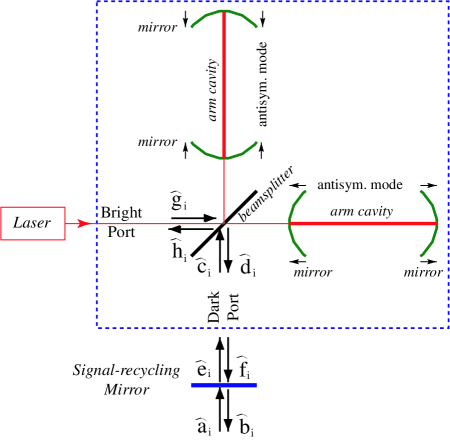
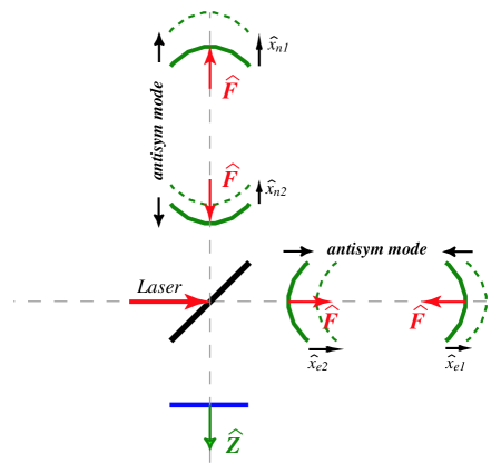
FIG. 4.: On the left panel we draw a SR interferometer, showing the antisymmetric mode of mirror motion (marked by arrows), the dark-port and SR optical fields $\widehat{a}_{i},\ldots,\widehat{f}_{i}$ and the bright-port fields $\widehat{g}_{i},\widehat{h}_{i}$, $i=1,2$. The conventional-interferometer optical scheme is contained inside the dashed box. In the right panel we identify the variables, $\widehat{x}\equiv\widehat{x}_{\rm antisym}=(\widehat{x}_{n1}-\widehat{x}_{n2})-(\widehat{x}_{e1}-\widehat{x}_{e2})$, $\widehat{Z}$ and $\widehat{F}$, describing the dynamics of the SR interferometer.

A Identifying the dynamical variables and their interactions

In gravitational-wave interferometers composed of equal-length arms (the optical configuration adopted by LIGO/VIRGO/GEO/TAMA), laser interferometry is used to monitor the displacement of the antisymmetric mode of the four arm-cavity mirrors induced by the passage of a gravitational wave (see Fig. 4).

Recently Kimble, Levin, Matsko, Thorne and Vyatchanin (KLMTV for short) [12] described a conventional (LIGO-I type) interferometer using a full quantum mechanical approach (see the optical scheme inside the dashed box in the left panel of Fig. 4). KLMTV [12] showed (as has long been known [31]) that in this kind of interferometer the antisymmetric mode of motion of the four arm-cavity mirrors and the dark-port sideband fields ($\widehat{c}_{i}$ and $\widehat{d}_{i}$ in Fig. 4) are decoupled from other degrees of freedom, i.e. from other modes of motion of the four arm-cavity mirrors and from the bright-port sideband fields ($\widehat{g}_{i}$ and $\widehat{h}_{i}$ in Fig. 4). As a consequence, the dynamics relevant to the output signal and the corresponding noise are described only by the antisymmetric mode of motion of the four arm-cavity mirrors and the dark-port sideband fields (see Appendix B of KLMTV [12] for details). This result remains valid for SR interferometers [13, 14]: we only need to include in the analysis all the optical fields inside the SR cavity, such as $\widehat{c}_{i}$, $\widehat{d}_{i}$, $\widehat{e}_{i}$ and $\widehat{f}_{i}$ [but not $\widehat{g}_{i}$ or $\widehat{h}_{i}$], and those outside the SR cavity, such as $\widehat{a}_{i}$ and $\widehat{b}_{i}$.

The coordinate of the antisymmetric mode of motion is defined by KLMTV [see Fig. 3 and Eq. (12) of Ref. [12], and the right panel of Fig. 4 in our paper] as:

$$\widehat{x}_{\rm antisym}\equiv(\widehat{x}_{n1}-\widehat{x}_{n2})-(\widehat{x}_{e1}-\widehat{x}_{e2})\,,$$ (54)

and we identify it with the dynamical variable $\widehat{x}$ introduced in Sec. II B [see Eq. (10)]. The output of the detector can be constructed from two independent output observables, the two quadratures $\widehat{b}_{1}$ and $\widehat{b}_{2}$ of the outgoing electromagnetic field immediately outside the SR mirror (see the left panel of Fig. 4). If a homodyne-detection read-out scheme is implemented, then the output is a linear combination of the two quadratures, that is

$$\widehat{b}_{\zeta}\equiv\sin\zeta\,\widehat{b}_{1}+\cos\zeta\,\widehat{b}_{2}\,,\quad\zeta={\rm const}\,,$$ (55)

which is a generic quadrature field. We thus identify the dynamical variable $\widehat{Z}$ introduced in Sec. II B [Eq. (8)] as:

$$\widehat{Z}_{\zeta}\equiv\widehat{b}_{\zeta}\,.$$ (56)

In particular, when $\zeta=\pi/2$ and $\zeta=0$ we have $\widehat{Z}_{1}\equiv\widehat{b}_{1}$ and $\widehat{Z}_{2}\equiv\widehat{b}_{2}$.

The radiation-pressure force acting on the arm-cavity mirrors, and coupled to the antisymmetric mode, can be directly related to the dark-port quadrature fields. This result was explicitly derived in Appendix B of KLMTV [12]. As a foundation for subsequent calculations, we shall summarize the main steps of their derivation: The force acting on each arm-cavity mirror is $2W/c$, where $W$ is the power circulating in each arm cavity, which is proportional to the square of the amplitude of the electric field propagating toward the mirror. In the arm cavities, the electric field can be decomposed into two parts: the carrier and the sideband fields. Introducing the carrier amplitude $C$ and the sideband quadrature operators $\widehat{s}_{1,2}$, we have

$$\widehat{E}(t)=C\cos\omega_{0}t+\cos\omega_{0}t\,\left[\int_{0}^{+\infty}\frac{d\Omega}{2\pi}\,e^{-i\,\Omega t}\,\widehat{s}_{1}+{\rm h.c.}\right]+\sin\omega_{0}t\,\left[\int_{0}^{+\infty}\frac{d\Omega}{2\pi}\,e^{-i\,\Omega t}\,\widehat{s}_{2}+{\rm h.c.}\right]\,,$$ (57)

where h.c. stands for Hermitian conjugate. (Note that by writing the carrier field as $C\cos\omega_{0}t$, we have adopted the convention used by KLMTV [12].) Taking the square of $\widehat{E}(t)$, we obtain

$$\widehat{E}^{2}(t) = {[\rm DC\;component]}+{[\rm high\;frequency\;component\;(>\!\omega_{0})]}$$ (58)

$$+ {C}\,\left[\int_{0}^{+\infty}\frac{d\Omega}{2\pi}\,e^{-i\,\Omega t}\,\widehat{s}_{1}+{\rm h.c.}\right]+(\rm quadratic\;terms\;in\;\widehat{s}_{1},\,\widehat{s}_{2})\,,$$ (59)

where we have used the fact that in the integral $\Omega<\omega_{0}$. The DC and $\omega_{0}\sim 10^{15}\,{\rm sec}^{-1}$ components are not in the detection band of GW interferometers, $10\,{\rm Hz}\leq\Omega/2\pi\leq 10^{4}\,{\rm Hz}$; in practice they will be counteracted by control systems. We also ignore the quadratic terms in Eq. (59), since they are much smaller than the linear terms. Thus, modulo a factor of proportionality, we obtain in the Fourier domain the following expression for the radiation-pressure force acting on each mirror:

$$\widehat{F}_{\rm RP}(\Omega)\propto C\,\widehat{s}_{1}(\Omega)\,.$$ (60)

As shown in Appendix B of Ref. [12], the in-cavity quadrature field $\widehat{s}_{1}$ is a combination of the incoming quadratures from both the dark and the bright ports. However, the contribution from the bright-port fields do not couple to the antisymmetric mode, so the force acting on the antisymmetric mode is due only to the incoming fields from the dark port. More specifically, in Sec. 4 of Appendix B of Ref. [12], KLMTV related the in-cavity carrier amplitude $C$ and the sideband quadrature $\widehat{s}_{1}$ (which they denoted by $\widehat{j}_{1}$ ) to the input carrier amplitude and ingoing dark-port quadrature $\widehat{c}_{1}$ (which they denoted by $\widehat{a}_{1}$). Although they did not give the explicit expression we need here for $\widehat{F}_{\rm RP}$, it is straightforward to recover it. Using the arrows indicated in the right panel of Fig. 4 as positive directions, we find

$$\widehat{F}_{\rm RP}=\sqrt{\frac{2I_{0}\hbar\omega_{0}}{\left(\Omega^{2}+\gamma^{2}\right)L^{2}}}\,e^{i\,\beta}\,\widehat{c}_{1},$$ (61)

where $\omega_{0}$ is the carrier laser frequency, $I_{0}$ is the carrier light power entering the beamsplitter, $2\beta=2\arctan{{\Omega}/{\gamma}}$ is the net phase gained by the sideband frequency $\Omega$ while in the arm cavity, $\gamma=Tc/4L$ is the half bandwidth of the arm cavity ($T$ is the power transmissivity of the input mirrors and $L$ is the length of the arm cavity). We identify the force $\widehat{F}_{\rm RP}$ with the dynamical variable $\widehat{F}$ introduced in Sec. II B [see Eq. (9)]:

$$\widehat{F}\equiv\widehat{F}_{\rm RP}=\sqrt{\frac{2I_{0}\hbar\omega_{0}}{\left(\Omega^{2}+\gamma^{2}\right)L^{2}}}\,e^{i\,\beta}\,\widehat{c}_{1}\,.$$ (62)

Applying Newton’s law to the four mirrors, we deduce

$$m\,\ddot{\widehat{x}}=4\widehat{F}+{\rm other\;forces}\,,$$ (63)

where “other forces” refer to forces not due to the optical-mechanical interaction, e.g., the force due to the gravitational wave and thermal forces. By identifying the reduced mass of the antisymmetric mode as $m/4$, we obtain that the coupling term in the total Hamiltonian (7) is $-\widehat{x}\,\widehat{F}$. [The reduced mass coincides with the effective mass of the probe $\mu$ introduced in Sec. II.]

Note that, by assuming the four forces acting on the arm-cavity mirrors are equal, we have made the approximation used by KLMTV [12] of disregarding the motion of the mirrors during the light’s round-trip time (quasi-static approximation).

B Free evolutions of test mass and optical field

In this section we derive the dynamics of the free probe and the detector, i.e. that of the antisymmetric mode of motion of the arm-cavity mirrors when there is no light in the arm cavities, and that of the optical fields when the arm-cavity mirrors are held fixed. The full, coupled dynamics will be discussed in the following section.

The mirror-endowed test masses are suspended from seismic isolation stacks and have free oscillation frequency $\sim\!1\,{\rm Hz}$. However, since we are interested in frequencies above $\sim\!10\,{\rm Hz}$ (below these frequencies the seismic noise is dominant), we can approximate the antisymmetric-mode coordinate as the coordinate of a free particle with (reduced) mass $m/4$ — as is also done by KLMTV [12]. Hence, its free evolution is given by

$$\widehat{x}^{(0)}(t)=\widehat{x}_{s}+\frac{4}{m}\,\widehat{p}_{s}\,t\,,$$ (64)

where $\widehat{x}_{s}$ and $\widehat{p}_{s}$ are the Schrödinger operators of the canonical coordinate and momentum of the mode. Inserting Eq. (64) into Eqs. (11), (17) and using the usual commutation relations $[\widehat{x}_{s},\widehat{p}_{s}]=i\hbar$, it is straightforward to derive

$$R_{xx}=-\frac{4}{m\Omega^{2}}\,.$$ (65)

As discussed in detail by BGKMTV [30], since at frequencies below $\raise 1.72218pt\hbox{$<$}\kern-8.00003pt\lower 2.6694pt\hbox{$\sim$}\,10$ Hz the data will be filtered out, the free evolution observable $\widehat{x}^{(0)}(t)$, whose Fourier component has support only at zero frequency (in a real interferometer it has support at the pendulum frequency $\sim\!1\,{\rm Hz}$), does not contribute to the output noise. For this reason, henceforth, we shall disregard the free-evolution observable $\widehat{x}^{(0)}(t)$ in the equations of motion describing the dynamics of GW interferometers.

Concerning the free detector (the light with fixed mirrors), we can solve its dynamics by expressing the various quantities in terms of the quadrature operators of the input field at the SR mirror, $\widehat{a}_{i}$, $i=1,2$ (see Fig. 4). For LIGO-II the input field will be in the vacuum state. All the quantum fluctuations affecting the output optical field $\widehat{b}_{i}$ are due to the vacuum fluctuations $\widehat{a}_{i}$ entering the interferometer from the SR mirror.

Through Eqs. (56), (62), we have already expressed $\widehat{Z}$ and $\widehat{F}$ in terms of the quadrature fields $\widehat{b}_{\zeta}$ and $\widehat{c}_{1}$; thus we need now to relate the latter to $\widehat{a}_{i}$, $i=1,2$, This can be done using Eqs. (2.11),(2.15)–(2.19) of Ref. [14], in the case of fixed mirrors. First, for the input-output relation at the beam splitter (see Fig. 4) we have

$$\widehat{d}_{1}=\widehat{c}_{1}\,e^{2i\beta}\,,\quad\quad\widehat{d}_{2}=\widehat{c}_{2}\,e^{2i\beta}\,,$$ (66)

which is obtained from Eq. (2.11) of Ref. [14], or Eq. (16) of Ref. [12] in the limit $I_{0}\rightarrow 0$ and $h\rightarrow 0$, i.e. when we neglect the effects of mirror motion under radiation pressure and gravitational waves. Second, propagating the quadrature fields inside the SR cavity, we obtain [see Eqs. (2.16), (2.17) of Ref. [14]]

$$\widehat{f}_{1}=(\widehat{d}_{1}\,\cos{\phi}-\widehat{d}_{2}\,\sin{\phi})\,,\quad \quad\widehat{f}_{2}=(\widehat{d}_{1}\,\sin{\phi}+\widehat{d}_{2}\,\cos{\phi})\,,$$ (67)

$$\widehat{e}_{1}=(\widehat{c}_{1}\,\cos{\phi}+\widehat{c}_{2}\,\sin{\phi})\,,\quad \quad\widehat{e}_{2}=(-\widehat{c}_{1}\,\sin{\phi}+\widehat{c}_{2}\,\cos{\phi})\,,$$ (68)

where $\phi\equiv[\omega_{0}l/c]_{{\rm mod}\;2\pi}$ is the phase gained by the carrier frequency $\omega_{0}$ traveling one-way in the SR cavity, and for simplicity we have neglected the tiny additional phase $\Phi\equiv{\Omega l}/{c}$ gained by the sideband frequency $\Omega/2\pi$ in the SR cavity. [The length of the SR cavity is typically $l\sim\!10\,{\rm m}$, hence $\Phi\ll 1$.] From the reflection/transmission relations at the SR mirror we derive [see Eqs. (2.18), (2.19) of Ref. [14]]

$$\widehat{e}_{1}=\tau\,\widehat{a}_{1}+\rho\,\widehat{f}_{1}\,,\quad\quad\widehat{e}_{2}=\tau\,\widehat{a}_{2}+\rho\,\widehat{f}_{2}\,,$$ (69)

$$\widehat{b}_{1}=\tau\,\widehat{f}_{1}-\rho\,\widehat{a}_{1}\,,\quad\quad\,\,\widehat{b}_{2}=\tau\,\widehat{f}_{2}-\rho\,\widehat{a}_{2}\,,$$ (70)

where $\tau$ and $\rho$ are the transmissivity and reflectivity of the SR mirror, with $\tau^{2}+\rho^{2}=1$. Solving Eqs. (66)–(70) and using Eq. (56), we obtain for the free-evolution operators

$$\widehat{Z}^{(0)}_{1}(\Omega)\equiv\left[\widehat{b}_{1}(\Omega)\right]_{\rm mirrors\;fixed} = \frac{e^{2i\beta}}{M_{0}}\left\{\left[\left(1+\rho^{2}\right)\,\cos 2\phi-2\rho\,\cos 2\beta\right]\,\widehat{a}_{1}-\tau^{2}\,\sin 2\phi\,\widehat{a}_{2}\right\}\,,$$ (71)

$$\widehat{Z}^{(0)}_{2}(\Omega)\equiv\left[\widehat{b}_{2}(\Omega)\right]_{\rm mirrors\;fixed} = \frac{e^{2i\beta}}{M_{0}}\left\{\tau^{2}\,\sin 2\phi\,\widehat{a}_{1}+\left[\left(1+\rho^{2}\right)\,\cos 2\phi-2\rho\,\cos 2\beta\right]\,\widehat{a}_{2}\right\}\,,$$ (72)

$$\left[\widehat{c}_{1}(\Omega)\right]_{\rm mirrors\;fixed} = \frac{\tau\left[\left(1-\rho\,e^{2i\beta}\right)\,\cos\phi\,\widehat{a}_{1}-\left(1+\rho\,e^{2i\beta}\right)\,\sin\phi\,\widehat{a}_{2}\right]}{M_{0}}\,$$ (73)

where we have defined,

$$M_{0}(\Omega) \equiv 1+\rho^{2}\,e^{4i\beta}-2\rho\,\cos 2\phi\,e^{2i\beta}\,=\left(1+2\rho\,\cos 2\phi+\rho^{2}\right)\,\frac{(\Omega-\Omega_{+})\,(\Omega-\Omega_{-})}{(\Omega+i\gamma)^{2}}\,,$$ (74)

and

$$\Omega_{\pm}=\frac{1}{1+2\rho\,\cos 2\phi+\rho^{2}}\,\left[\pm 2\rho\,\gamma\,\sin 2\phi-i\gamma\,(1-\rho^{2})\right]\,.$$ (75)

Note that $\widehat{Z}^{(0)}_{\zeta}$ can be computed from Eqs. (71), (72) by taking the linear combination of $\widehat{Z}^{(0)}_{1}$ and $\widehat{Z}^{(0)}_{2}$, in the manner of Eqs. (55), (56). From Eqs. (62) and (73) we obtain for the free-evolution radiation-pressure force:

$$\widehat{F}^{(0)}(\Omega) = \tau\,\sqrt{\frac{2I_{0}\hbar\omega_{0}}{\left(\Omega^{2}+\gamma^{2}\right)L^{2}}}\,\frac{e^{i\,\beta}}{M_{0}}\left[\left(1-\rho\,e^{2i\beta}\right)\,\cos\phi\,\widehat{a}_{1}-\left(1+\rho\,e^{2i\beta}\right)\,\sin\phi\,\widehat{a}_{2}\right]\,.$$ (76)

Using Eqs. (71), (72) and (76), and the fact that $\zeta$ is frequency independent, we have explicitly checked that the susceptibilities of the free-evolution operators, $\widehat{Z}_{\zeta}^{(0)}$ and $\widehat{F}^{(0)}$, satisfy the necessary and sufficient conditions LQM, given in Sec. II C, which define a linear quantum-measurement system with output $\widehat{Z}$. More specifically, using the commutation relations among the quadrature fields $\widehat{a}_{1}$ and $\widehat{a}_{2}$ [Eqs. (7a), (7b) of Ref. [12]], namely

$$[\widehat{a}_{1},\widehat{a}_{2^{\prime}}^{\dagger}]=-[\widehat{a}_{2},\widehat{a}_{1^{\prime}}^{\dagger}]=2\pi\,i\,\delta(\Omega-\Omega^{\prime})\,,$$ (77)

$$[\widehat{a}_{1},\widehat{a}_{1^{\prime}}^{\dagger}]=0=[\widehat{a}_{1},\widehat{a}_{1^{\prime}}]\,,\quad\quad[\widehat{a}_{2},\widehat{a}_{2^{\prime}}^{\dagger}]=0=[\widehat{a}_{2},\widehat{a}_{2^{\prime}}]\,,$$ (78)

we have derived that

$$R_{Z_{\zeta}Z_{\zeta}}=0=R_{FZ_{\zeta}}\,;$$ (79)

and we have also derived that

$$R_{FF}(\Omega) = \frac{2I_{0}\,\omega_{0}}{L^{2}}\,\frac{\rho\,\sin 2\phi}{1+2\rho\,\cos 2\phi+\rho^{2}}\,\frac{1}{(\Omega-\Omega_{+})\,(\Omega-\Omega_{-})}\,,$$ (80)

$$R_{Z_{1}F}(\Omega) = -i\,\sqrt{\frac{2I_{0}\,\omega_{0}}{\hbar\,L^{2}}}\,\frac{\tau\sin\phi}{1+2\rho\,\cos 2\phi+\rho^{2}}\,\frac{(1-\rho)\,\Omega+i(1+\rho)\,\gamma}{(\Omega-\Omega_{+})\,(\Omega-\Omega_{-})}\,,$$ (81)

$$R_{Z_{2}F}(\Omega) = i\,\sqrt{\frac{2I_{0}\,\omega_{0}}{\hbar\,L^{2}}}\,\frac{\tau\cos\phi}{1+2\rho\,\cos 2\phi+\rho^{2}}\,\frac{(1+\rho)\,\Omega+i(1-\rho)\,\gamma}{(\Omega-\Omega_{+})\,(\Omega-\Omega_{-})}\,,$$ (82)

$$R_{Z_{\zeta}{F}}(\Omega)=R_{Z_{1}F}(\Omega)\,\sin\zeta+R_{Z_{2}F}(\Omega)\,\cos\zeta\,.$$ (83)

In actuality the commutation relations (77), (78) are approximate expressions for $\Omega\ll\omega_{0}$. However, this is a good approximation since the sideband frequency $\Omega/2\pi$ varies over the range $10-10^{4}\,{\rm Hz}$, which is ten orders of magnitude smaller than $\omega_{0}/2\pi\!\sim\!10^{14}\,{\rm Hz}$. If we had used the exact commutation relations (see Caves and Schumaker [32] or Eqs. (2.4), (2.5) of Ref. [14]), we would still have $R_{FZ_{\zeta}}=0$, but we would have correction terms in the other susceptibilities. In particular, $R_{Z_{\zeta}Z_{\zeta}}$ would not vanish, but would instead be on the order of $\Omega/\omega_{0}$. These issues are discussed in the Appendix of Ref. [14].

Before ending this section we want to discuss the resonant features of the free-evolution optical fields, which originally motivated the Signal Recycling (SR) [4, 5, 6] and Resonant Sideband Extraction (RSE) schemes [7, 8, 9]. By definition a resonance is an infinite response to a driving force acting at a certain (complex) frequency. Mathematically, it corresponds to a pole of the Fourier-domain susceptibility at that (complex) frequency. From Eqs. (80)–(83) we deduce that $R_{FF}$ and $R_{Z_{\zeta}F}$ have only two poles $\Omega_{\pm}$, given by Eq. (75), which are the two complex resonant frequencies of the free optical fields, Eqs. (71), (72). The corresponding eigenmodes are of the form $e^{-t/\tau_{\rm decay}}\,e^{-i\,\Omega_{\rm osc}\,t}$, with oscillation frequency

$$\Omega_{{\rm osc}\pm}={\Re}(\Omega_{\pm})=\pm\frac{2\rho\,\gamma\,\sin 2\phi}{1+2\rho\,\cos 2\phi+\rho^{2}}\,,$$ (84)

and decay time

$$\tau_{\rm decay}=-\frac{1}{{\Im}(\Omega_{\pm})}=\frac{1+2\rho\,\cos 2\phi+\rho^{2}}{\gamma\,(1-\rho^{2})}\,.$$ (85)

This oscillation frequency and decay time give information on the frequency of perturbations to which the optical fields are most sensitive, and on the time these perturbations last in the interferometer before leaking out. Let us focus on several limiting cases:

• For $\rho=0$, i.e. the case of a conventional (LIGO-I type) of interferometer, we have $\Omega_{\rm osc}=0$ and $\tau_{\rm decay}=1/\gamma$. Thus, there is no oscillation, while the decay time $1/\gamma$ of the entire interferometer is just the storage time of the arm cavity.

• For $\rho\rightarrow 1$, i.e. when the SR optical system is nearly closed, we have $\Omega_{\rm osc}=\pm\gamma\tan\phi$ and $\tau_{\rm decay}\rightarrow+\infty$, which corresponds to a pure oscillation. Noticing that for sideband fields with frequency $\Omega/2\pi$, the phase gained in the arm cavity is $2\beta=2\arctan{\Omega/\gamma}$ and the phase gained during a round trip in the SR cavity is $2\phi=2\omega_{0}l/c$, we obtain that $\Omega_{\rm osc}$ is just the frequency at which the total round-trip phase in the entire cavity (arm cavity + SR cavity) is $2\pi n$, with $n$ an integer.

• For $0<\rho<1$ and $\phi=0$, we get $\Omega_{\rm osc}=0$ and $\tau_{\rm decay}=({1+\rho})/[{\gamma\,(1-\rho)}]>{1}/{\gamma}$. This is the so-called tuned SR configuration [4, 5, 6], where the sideband fields remain in the inteferometer for a time longer than the storage time of the arm cavities [cf. (i)].

• For $0<\rho<1$ and $\phi=\pi/2$, we get $\Omega_{\rm osc}=0$ and $\tau_{\rm decay}=({1-\rho})/[{\gamma\,(1+\rho)}]<{1}/{\gamma}$. This is the so-called tuned RSE configuration [7, 8, 9], where the sideband fields remain in the interferometer for a time shorter than the storage time of the arm cavities [cf. (i)].

C Coupled evolution of test mass and optical field: ponderomotive rigidity

In Sec. II B we have solved the equations of motion for a generic quantum-measurement device by expressing the full-evolution operators in terms of the free-evolution operators [see Eqs. (21)–(23)]. Using the free-evolution optical-field operators (71), (72) and (76) and the optical-field susceptibilities (80)–(83), along with the susceptibility of the antisymmetric mode (65), we can now obtain the full evolution of the antisymmetric mode $\widehat{x}^{(1)}$ and that of the output optical field $\widehat{Z}^{(1)}_{\zeta}$ for a SR interferometer. In Ref. [14], we evaluated the output quadrature fields by a slightly different method, introduced by KLMTV [12]. However, the approach followed in this paper provides the output field in a more straightforward way, and gives a clearer understanding of the interferometer dynamics. Moreover, we think this method is more convenient when the optical configuration of the interferometer is rather complex.

We start by investigating the interaction between the probe and the detector. The equations that couple the various quantities $\widehat{x}$, $\widehat{F}$ and $\widehat{Z}$ are [Eqs. (18)–(20)]:

$$\widehat{Z}_{\zeta}^{(1)}(\Omega) = \widehat{Z}_{\zeta}^{(0)}(\Omega)+R_{Z_{\zeta}F}(\Omega)\,\widehat{x}^{(1)}(\Omega)\,,$$ (86)

$$\widehat{F}^{(1)}(\Omega) = \widehat{F}^{(0)}(\Omega)+R_{FF}(\Omega)\,\widehat{x}^{(1)}(\Omega)\,,$$ (87)

$$\widehat{x}^{(1)}(\Omega) = R_{xx}(\Omega)\,[G(\Omega)+\widehat{F}^{(1)}(\Omega)]\,.$$ (88)

In these equations, we have made explicit the dependence on the gravitational force $G(\Omega)=-(m/4)\,\Omega^{2}\,h(\Omega)$ [see also Eq. (16)] and have neglected the free evolution operator $\widehat{x}^{(0)}$ (see the discussion at the beginning of Sec. III B).

Equation (88) is the equation of motion of the antisymmetric mode under the GW force $G$ and the radiation-pressure force $\widehat{F}$, with response function $R_{xx}$. Equations (86) and (87) are the equations of motion of the optical fields $\widehat{Z}_{\zeta}$ and $\widehat{F}$ under the modulation of the antisymmetric mode of motion of the four arm-cavity mirrors $\widehat{x}$, with response functions $R_{Z_{\zeta}F}(\Omega)$ and $R_{FF}(\Omega)$, respectively.

The optical-mechanical interaction in a conventional interferometer ($\rho=0$ and $\phi=0$) was analyzed by KLMTV in Ref. [12]. Here we summarize only the main features. Inside the arm cavity the electric field is [see Eq. (57)]

$$\widehat{E}(t) \propto C\cos\omega_{0}t+\widehat{S}_{1}(t)\cos\omega_{0}t+\widehat{S}_{2}(t)\sin\omega_{0}t\,,$$ (89)

$$\approx C\left[1+\frac{\widehat{S}_{1}(t)}{C}\right]\cos\left[\omega_{0}t-\frac{\widehat{S}_{2}(t)}{C}\right]\,,$$ (90)

with

$$\widehat{S}_{j}(t)=\int_{0}^{+\infty}\frac{d\Omega}{2\pi}\,e^{-i\,\Omega\,t}\,\widehat{s}_{j}+{\rm h.c.}\,,\quad\quad j=1,2\,,$$ (91)

where in Eq. (90) we have assumed that the sideband amplitudes are much smaller than the carrier amplitude. From Eq. (90) we infer that the sideband fields $\widehat{S}_{1}$ and $\widehat{S}_{2}$ modulate the amplitude and the phase of the carrier field. If the arm-cavity mirrors are not moving, then it is easy to deduce that $\widehat{b}_{1}\propto\widehat{s}_{1}\propto\widehat{a}_{1}$ and $\widehat{b}_{2}\propto\widehat{s}_{2}\propto\widehat{a}_{2}$ (see Fig. 4). Thus, given our conventions for the quadratures, we can refer to $\widehat{s}_{1}$, $\widehat{a}_{1}$ and $\widehat{b}_{1}$ as amplitude quadratures, and $\widehat{s}_{2}$, $\widehat{a}_{2}$ and $\widehat{b}_{2}$ as phase quadratures in the present case of a conventional interferometer. When the arm-cavity mirrors move, their motion modulates the phase of the carrier field, pumping part of it into the phase quadrature $\widehat{S}_{2}(t)$, and thus into $\widehat{b}_{2}$ [see Appendix B of Ref. [12], especially Eq. (B9a)]. As a consequence $R_{Z_{2}F}\neq 0$ but $R_{Z_{1}F}=0$. On the other hand, the radiation-pressure force acting on the arm-cavity mirrors is determined by the amplitude modulation $\widehat{S}_{1}(t)$ and does not respond to the motion of the arm-cavity mirrors; thus $R_{FF}=0$.

Let us now analyze a SR interferometer. As pointed out above, the antisymmetric mode of motion of the arm-cavity mirrors, $\widehat{x}$, only appears in the phase quadrature $\widehat{d}_{2}$. [Note that now $\widehat{c}_{i}$ and $\widehat{d}_{i}$ take the place of $\widehat{a}_{i}$ and $\widehat{b}_{i}$ in the above analysis of conventional interferometers.] Schematically,

$$\left(\begin{array}[]{c}\widehat{c}_{1}\\ \widehat{c}_{2}\end{array}\right)\stackrel{{\scriptstyle\rm arm\atop cavity}}{{\longrightarrow}}e^{i\,({\rm phase})}\left(\begin{array}[]{c}\widehat{c}_{1}\\ \widehat{c}_{2}\end{array}\right)+\left(\begin{array}[]{c}0\\ \widehat{x}\end{array}\right)\Leftrightarrow\left(\begin{array}[]{c}\widehat{d}_{1}\\ \widehat{d}_{2}\end{array}\right)\,.$$ (92)

Because of the presence of the SR mirror, part of the field coming out from the beamsplitter is reflected by the SR mirror and fed back into the arm cavities. Due to the propagation inside the SR cavity, the outgoing amplitude/phase quadrature fields at the beamsplitter, $\widehat{d}_{1,2}$, get rotated [see Eqs. (67), (68)]. Moreover, whereas part of the light leaks out from the SR mirror, contributing to the output field, some vacuum fields leak into the SR cavity from outside [see Eqs. (69), (70)]. When the light reflected by the SR mirror, along with the vacuum fields that have leaked in, reaches the beamsplitter again, the rotation angle is $2\phi\,$. Schematically, we can write

$$\left(\begin{array}[]{l}\widehat{d}_{1}\\ \widehat{d}_{2}\end{array}\right)\stackrel{{\scriptstyle\rm SR\atop cavity}}{{\longrightarrow}}\rho\left(\begin{array}[]{cc}\cos 2\phi&-\sin 2\phi\\ \sin 2\phi&\cos 2\phi\end{array}\right)\left(\begin{array}[]{l}\widehat{d}_{1}\\ \widehat{d}_{2}\end{array}\right)+\tau\left({\rm vacuum\;fields\atop from\;outside}\right)\Leftrightarrow\left(\begin{array}[]{l}\widehat{c}_{1}\\ \widehat{c}_{2}\end{array}\right)\,,$$ (93)

where $\rho$ and $\tau$ are the amplitude reflectivity and transmissivity of the SR mirror.

In the particular case of $\phi=0\;{\rm or}\;{\pi}/{2}$, namely the tuned SR/RSE configurations [6, 7, 8, 9], the rotation matrix in Eq. (93) is diagonal. Since $\widehat{x}$ appears only in $\widehat{d}_{2}$ [see Eq. (92)], the fact that the propagation matrix is diagonal guarantees that $\widehat{x}$ remains only in the quadratures $\widehat{d}_{2}$ and $\widehat{c}_{2}$. As a result, the radiation-pressure force, which is proportional to $\widehat{c}_{1}$ [see Eq. (62)], is not affected by the antisymmetric mode of motion, and $R_{FF}=0$ [see Eq. (80)] as in conventional interferometers. Moreover, since the quadratures at the beamsplitter $\widehat{d}_{1,2}$ are rotated by an angle of $\phi$ when they reach the SR mirror [see Eq. (67)], the information on the motion of the arm-cavity mirrors is contained only in the output quadrature $\widehat{b}_{2}$ for $\phi=0$ and $\widehat{b}_{1}$ for $\phi={\pi}/{2}$. Therefore $R_{Z_{1}F}=0$ for $\phi=0$ and $R_{Z_{2}F}=0$ for $\phi={\pi}/{2}$, as obtained directly from Eqs. (81), (82).

For a generic configuration with $\phi\neq 0\;{\rm or}\;{\pi}/{2}$, which is often referred to as the detuned case [6], $\widehat{x}$ appears in both the quadratures $\widehat{c}_{1,2}$ as a consequence of the nontrivial rotation in Eq. (93). Thus the radiation-pressure force and both the output quadratures respond to $\widehat{x}$, i.e. $R_{FF}\neq 0$ and $R_{Z_{\zeta}F}\neq 0$ for all $\zeta$, as can be seen from Eqs. (80)–(82).

Before ending this section let us make some remarks. When $R_{FF}=0$, as occurs in conventional interferometers and the tuned SR/RSE configurations, we infer from Eqs. (65), (87) and (88) that

$$-\frac{m}{4}\,\Omega^{2}\,\widehat{x}^{(1)}(\Omega)=G(\Omega)+\widehat{F}^{(0)}(\Omega)\,.$$ (94)

This means that the antisymmetric mode of motion of the four arm-cavity mirrors behaves as a free test mass subject to the GW force $G(\Omega)$ and the fluctuating radiation-pressure force $\widehat{F}^{(0)}$. It is well known that for such systems the Heisenberg uncertainty principle imposes a limiting noise spectral density $S_{h}^{\rm SQL}=8\hbar/(m\Omega^{2}L^{2})$ for the dimensionless gravitational-wave signal $h(t)=\Delta L/L$ [35]. This limiting noise spectral density is called the standard quantum limit (SQL) for GW interferometers, and LIGO/VIRGO/GEO/TAMA interferometers can beat this SQL only if correlations among the optical fields are introduced [18, 19, 12, 13, 14].

When $R_{FF}\neq 0$, Eqs. (65), (87) and (88) give

$$-\frac{m}{4}\,\Omega^{2}\,\widehat{x}^{(1)}(\Omega)=G(\Omega)+\widehat{F}^{(0)}(\Omega)+R_{FF}(\Omega)\,\widehat{x}^{(1)}(\Omega)\,.$$ (95)

Thus the antisymmetric mode of motion of the four arm-cavity mirrors is not only disturbed randomly by the fluctuating force $\widehat{F}^{(0)}$, but also, and more fundamentally, is subject to a linear restoring force with a frequency-dependent rigidity (or “spring constant”) $K(\Omega)=-R_{FF}(\Omega)\neq 0$, generally called a ponderomotive rigidity [20]. This phenomenon was originally analyzed in “optical-bar” GW detectors by Braginsky, Khalili and colleagues, where the ponderomotive rigidity affects the internal mirror, i.e. an intra-cavity meter which couples the two resonators with end-mirror–endowed test masses [20]. Hence, SR interferometers do not monitor the displacements of a free test mass but instead that of a test mass subject to a force field $\widehat{F}_{\rm res}(\Omega)=-K(\Omega)\,\widehat{x}^{(1)}(\Omega)$. This suggests that the SQL, derived from the monitoring of a free test mass, is irrelevant for detuned SR interferometers. Indeed, in Ref. [13, 14] we found that there exists a region of the parameter space $\rho$, $\phi$ and $I_{0}$ for which the quantum noise curves can beat the SQL by roughly a factor of two over a bandwidth $\Delta f\!\sim\!f$.

IV Dynamics of Signal recycled interferometers: Resonances and Instabilities

In the previous section we have shown that in a SR interferometer the four arm-cavity mirrors are subject to a frequency dependent restoring force. Thus we expect the mirrors’ motion be characterized by resonances and possible instabilities. In Refs. [13, 14], we have identified those resonances by evaluating the input-output relation for the quadrature fields $\widehat{b}_{i}$ ($\widehat{a}_{i},h$). In this section, by using the dynamics of the whole system composed of the optical fields and the mirrors, we shall investigate in more detail the features of those resonances and instabilities.

A Physical origins of the two pairs of resonances

Let us first seek a qualitative understanding of the resonances. In Fig. 5 we draw the amplitude and the phase of the ponderomotive rigidity $R_{FF}$, given by Eq. (80), for a typical choice of LIGO-II parameters: $\phi={\pi}/{2}-0.47$, $\rho=0.9$ and $I_{0}\simeq 10^{4}\,{\rm W}$. The amplitude and phase of $R_{FF}$ resemble those of the response function of a damped harmonic oscillator, except for the fact that the phase of $R_{FF}$ is reversed. From Fig. 5 we infer that when the frequency $f=\Omega/2\pi$ is small, $|R_{FF}|$ is almost constant, while the phase is nearly $-180^{\circ}$. Thus in this frequency region the spring constant is approximately a constant positive number $\sim\!K(\Omega=0)=-R_{FF}(\Omega=0)>0$. However, $K(\Omega=0)$ is positive only if $0<\phi<{\pi}/{2}$, while for ${\pi}/{2}<\phi<\pi$ the spring constant at low frequencies is negative. As a consequence, for $\pi/2<\phi<\pi$, there is a non-oscillating instability, namely a pair of complex-conjugate purely imaginary resonant frequencies. [Note that because the SR-interferometer dynamics is invariant under the transformation $\phi\rightarrow\phi+\pi$ [14], we can restrict ourselves to $0\leq\phi\leq\pi$.]

For larger $f=\Omega/2\pi$, $K(\Omega)=-R_{FF}(\Omega)$ has a resonant peak centered at $\Omega=\Omega_{\rm osc}$, with width $\sim\!1/\tau_{\rm decay}$ [see Eqs. (84), (85)].

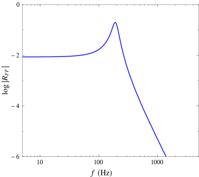
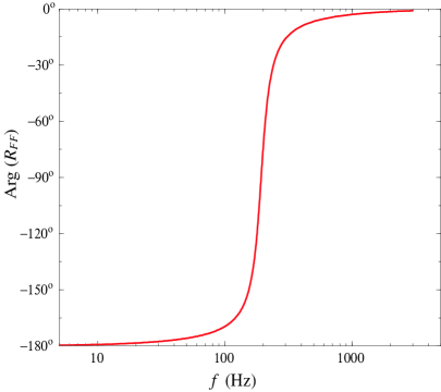
FIG. 5.: Amplitude (on the left panel) and phase (on the right panel) of $R_{FF}$ as a function of the sideband frequency $f=\Omega/2\pi$ for $\phi={\pi}/{2}-0.47$, $\rho=0.9$ and $I_{0}\simeq 10^{4}$ W. Note that the amplitude of $R_{FF}$ is shown in arbitrary unit.

Hence, the dynamics of the system composed of the optical field and the arm-cavity mirrors in a SR interferometer is analogous to the dynamics of a massive spring, with an internal mode, attached to a test mass. When the test mass moves at low frequency, i.e. $\Omega\ll\Omega_{\rm osc}$, the internal configuration of the spring has time to keep up with its motion and it remains uniform, providing a linear restoring force which induces a pair of resonances at frequencies $\Omega_{\rm mech}=\pm\sqrt{{4K(\Omega\ll\Omega_{\rm osc})}/{m}}\!\sim\!\pm\sqrt{{4K(\Omega=0)}/{m}}$.

When the test mass moves at high frequency, the internal mode of the spring is excited, providing another pair of resonances to the system. Inserting the equation of motion (88) of $\widehat{x}$ and the expression for $R_{FF}$, Eq. (80), into the equation of motion (87) of $\widehat{F}$, we obtain

$$-(\Omega-\Omega_{+})\,(\Omega-\Omega_{-})\,\widehat{F}^{(1)}(\Omega)={\rm driving\;terms}+\frac{4}{m\Omega^{2}}\,\frac{2I_{0}\omega_{0}}{L^{2}}\,\frac{\rho\sin 2\phi}{1+2\rho\cos 2\phi+\rho^{2}}\,\widehat{F}^{(1)}(\Omega)\,.$$ (96)

In the absence of the SR mirror, i.e. for $\rho=0$, the term proportional to $\widehat{F}^{(1)}$ on the RHS of Eq. (96) vanishes, and the optical field is characterized by the two resonant frequencies $\Omega_{\pm}$ given by Eq. (75). By contrast, when the SR mirror is present, the term proportional to $\widehat{F}^{(1)}$ on the RHS of Eq. (96) shifts the resonant frequencies away from the values $\Omega_{\pm}$.

In conclusion, the dynamics of SR interferometers is characterized by two (pairs of) resonances with different origin: the (pair of) resonances at low frequency have a “mechanical” origin, coming from the linear restoring force due to the ponderomotive rigidity; the (pair of) resonances at higher frequency have an “optical” origin. Because of the motion of the arm-cavity mirrors the optical resonant frequencies get shifted away from the free-evolution SR resonant frequencies $\Omega_{\pm}$. In this sense we can regard the SR interferometer as an “optical spring” [See Fig. 6].

FIG. 6.: The SR-interferometer dynamics resembles the dynamics of a massive spring with one internal oscillation mode (and damping) attached to a test mass. The overall dynamical system is characterized by two pairs of resonances.

B Quantitative investigation of the resonances

Equations (86)–(88) describe the coupled evolution of the dynamical variables $\widehat{x}$, $\widehat{F}$ and $\widehat{Z}$:

$$\widehat{x}^{(1)}(\Omega) = \frac{R_{xx}(\Omega)}{1-R_{xx}(\Omega)\,R_{FF}(\Omega)}\,\left[G(\Omega)+\widehat{F}^{(0)}(\Omega)\right]\,,$$ (97)

$$\widehat{F}^{(1)}(\Omega) = \frac{1}{1-R_{xx}(\Omega)\,R_{FF}(\Omega)}\,\left[\widehat{F}^{(0)}(\Omega)+R_{FF}(\Omega)\,R_{xx}(\Omega)G(\Omega)\right]\,,$$ (98)

$$\widehat{Z}_{\zeta}^{(1)}(\Omega) = \widehat{Z}^{(0)}_{\zeta}(\Omega)+\frac{R_{Z_{\zeta}F}(\Omega)\,R_{xx}(\Omega)}{1-R_{xx}(\Omega)\,R_{FF}(\Omega)}\,\left[G(\Omega)+\widehat{F}^{(0)}(\Omega)\right]\,.$$ (99)

Let us first analyze these equations in the low–laser-power limit, which has long been considered in the literature for the SR/RSE schemes [4, 5, 6, 7, 8, 9] and has recently been tested experimentally [10, 11]. For LIGO-II [3] low–laser-power limit corresponds to $I_{0}\ll 10^{4}\,{\rm W}$. Using Eqs. (80)–(83), and the fact that $\widehat{Z}_{\zeta}^{(0)}$ does not depend on $I_{0}$, and $\widehat{F}^{(0)}\propto\sqrt{I_{0}}$ [see Eqs. (71), (72) and (76)], we deduce that $R_{FF}\propto I_{0}$ and $R_{Z_{\zeta}F}\propto\sqrt{I_{0}}$. Therefore, for very low laser power, if we restrict ourselves only to terms up to the order of $\sqrt{I_{0}}$, we can reduce Eq. (99) to:

$$\left[\widehat{Z}_{\zeta}^{(1)}(\Omega)\right]_{\rm low\;power}=\widehat{Z}_{\zeta}^{(0)}(\Omega)+R_{Z_{\zeta}F}(\Omega)\,R_{xx}(\Omega)\,G(\Omega)\,,$$ (100)

which says that the response of $\widehat{Z}_{\zeta}^{(1)}$ to the GW force $G$ is given by the product of $R_{xx}$, the response of $\widehat{x}$ to $G$, times $R_{Z_{\zeta}F}$, the response of $\widehat{Z}_{\zeta}$ to $\widehat{F}$. Hence, for low laser power the dynamics is characterized by four decoupled resonant frequencies: two of them, $\Omega^{2}=0$ (degenerate), are those of the free test mass as embodied in $R_{xx}$; the other two, $\Omega=\Omega_{\pm}$ [see Eq. (75)], are those of the free-evolution optical fields as embodied in $R_{Z_{\zeta}F}$. As was discussed in Sec. II B, when the imaginary part of the resonant frequency is negative (positive) the mode is stable (unstable). Therefore the decoupled “mechanical” resonances $\Omega^{2}=0$ are marginally stable, while the decoupled “optical” resonances $\Omega_{\pm}$ are stable. [We remind the reader that $\Im(\Omega_{\pm})<0$.]

If we increase the laser power sufficiently, the effect of the radiation pressure is no longer negligible, and from Eqs. (97)–(99) we derive the following condition for the resonances:

$$\frac{R_{xx}(\Omega)\,R_{Z_{\zeta}F}(\Omega)}{1-R_{xx}(\Omega)\,R_{FF}(\Omega)}\rightarrow+\infty\,$$ (101)

which simplifies to,

$$\Omega^{2}\,(\Omega-\Omega_{+})\,(\Omega-\Omega_{-})+\frac{I_{0}\,\gamma^{3}}{2I_{\rm SQL}}\,(\Omega_{+}-\Omega_{-})=0\,.$$ (102)

In these equations we have adopted as a reference light power $I_{\rm SQL}\equiv{m\,L^{2}\,\gamma^{4}}/{4\omega_{0}}$, introduced by KLMTV [12]; this is the light power at the beamsplitter needed by a conventional interferometer to reach the SQL at $\Omega=\gamma$. Because of the presence of the term proportional to $I_{0}$ in Eq. (102), $\Omega^{2}=0$ and $\Omega=\Omega_{\pm}$ are no longer the resonant frequencies of the coupled SR dynamics.

If the laser power is not very high, we expect the roots of Eq. (102) to differ only slightly from the decoupled ones. Let us then apply a perturbative analysis. Concerning the double roots $\Omega^{2}=\Omega_{0}^{2}=0$, working at leading order in the frequency shift $\Delta\Omega_{0}=\Omega-\Omega_{0}=\Omega$, we derive

$$(\Delta\Omega_{0})^{2}=-\frac{I_{0}\,\gamma^{3}}{2I_{\rm SQL}}\,\frac{(\Omega_{+}-\Omega_{-})}{\Omega_{+}\,\Omega_{-}}=\frac{I_{0}}{I_{\rm SQL}}\,\frac{(2\rho\,\gamma^{2}\,\sin 2\phi)\,(1+2\rho\,\cos 2\phi+\rho^{2})}{4\rho^{2}\,\sin^{2}2\phi+(1-\rho^{2})^{2}}\,.$$ (103)

If the SR detuning phase lies in the range $0<\phi<\pi/2$, then $(\Delta\Omega_{0})^{2}$ is always positive. Hence, at leading order, the initial double zero resonant frequency $\Omega^{2}=0$ splits into two real resonant frequencies having opposite signs and proportional to $(I_{0}/I_{\rm SQL})^{1/2}\,\gamma$. The imaginary parts of these resonant frequencies appear only at the next to leading order, and it turns out (as discussed later on in this section) that they always increase (becoming more positive) as $I_{0}/I_{\rm SQL}$ grows, generating instabilities.

If the SR detuning phase lies in the range $\pi/2<\phi<\pi$, then at leading order $(\Delta\Omega_{0})^{2}$ is negative, and we get two complex-conjugate purely imaginary roots. The system is therefore characterized by a non-oscillating instability.

Regarding the roots $\Omega=\Omega_{\pm}$, we can expand Eq. (102) with respect to $\Delta\Omega_{\pm}=\Omega-\Omega_{\pm}$. A simple calculation gives

$$\Delta\Omega_{\pm}=\mp\frac{I_{0}\,\gamma^{3}}{2I_{\rm SQL}}\,\frac{1}{(\Omega_{\pm})^{2}}\,.$$ (104)

Using Eq. (75) we find that

$$\Re(\Delta\Omega_{\pm})=\mp\frac{I_{0}\,\gamma}{2I_{\rm SQL}}\,\frac{[4\rho^{2}\,\sin^{2}2\phi-(1-\rho^{2})^{2}]\,(1+2\rho\,\cos 2\phi+\rho^{2})^{2}}{[4\rho^{2}\,\sin^{2}2\phi+(1-\rho^{2})^{2}]^{2}}\,,$$ (105)

$$\Im(\Delta\Omega_{\pm})=-\frac{I_{0}}{I_{\rm SQL}}\,\frac{[2\rho\,\gamma\,\sin 2\phi\,(1-\rho^{2})]\,(1+2\rho\,\cos 2\phi+\rho^{2})^{2}}{[4\rho^{2}\,\sin^{2}2\phi+(1-\rho^{2})^{2}]^{2}}\,.$$ (106)

This says that, if the SR detuning phase lies in the range $0<\phi<\pi/2$, then $\Im(\Delta\Omega_{\pm})$ always decreases (becoming more negative) as $I_{0}/I_{\rm SQL}$ increases. Hence, the imaginary parts of the resonant frequencies are pushed away from the real $\Omega$ axis, i.e. the system remains stable. On the other hand, $\Re(\Delta\Omega_{\pm})$ may either increase or decrease as $I_{0}/I_{\rm SQL}$ grows. If $\pi/2<\phi<\pi$ then the imaginary parts become less negative as the laser power increases, so the system becomes less stable.

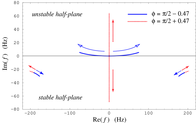
FIG. 7.: Shift of the resonances in a SR interferometer induced by the radiation pressure force as $I_{0}$ increases from $\sim\!0$ up to $I_{\rm SQL}$. This figure is drawn for a SR mirror reflectivity $\rho=0.9$.

Note that, although turning up the laser power drives the optical resonant frequencies away from their nonzero values $\Omega_{\pm}$, their changes are very small or comparable to their original values. By contrast, the mechanical resonant frequencies move away from zero; hence their motion is very significant. In this sense, as the laser power increases, the mechanical (test-mass) resonant frequencies move faster than the optical ones. This fact can also be understood by observing that $\Delta\Omega_{0}$ is proportional to the square root of $I_{0}$, while $\Delta\Omega_{\pm}$ is proportional to $I_{0}$ itself. For the optical configurations of interest for LIGO-II, we found [14] that when we increase the laser power from $I_{0}=0$ to $I_{0}=I_{\rm SQL}$, the optical resonant frequencies stay more or less close to their original values while the mechanical ones, which start from zero at $I_{0}=0$, move into the observation band of LIGO-II as $I_{0}\rightarrow I_{\rm SQL}$.

To get a more intuitive idea of the shift in the resonant frequencies for high laser power, we have explored the resonant features numerically. In Fig. 7 we plot the trajectories of the resonant frequencies when $I_{0}$ varies from $\sim\!0$ to $I_{\rm SQL}$ (the arrows indicate the directions of increasing power), for two choices of SR parameters: $\rho=0.9$, and $\phi=\pi/2\mp 0.47$, for which the decoupled resonant frequencies $\Omega_{\pm}$ coincide. The behaviours of the optical resonant frequencies under an increase of the power agree with the conclusion of the perturbative analysis deduced above. For $\phi=\pi/2-0.47$, or more generally for $0<\phi<\pi/2$, the imaginary part of the optical resonant frequency becomes more negative when the laser power increases, and the resonance becomes more stable; for $\phi=\pi/2-0.47$, or generically for $\pi/2<\phi<\pi$, the imaginary part becomes slightly less negative when the laser power increases. The behavior of the mechanical resonance is particularly interesting. For $\phi=\pi/2-0.47$, or generically for $0<\phi<\pi/2$, and for very low laser power $I_{0}$ the two resonant frequencies separate along the real axis, as anticipated by the perturbative analysis. Moreover, as $I_{0}$ increases they both gain a positive imaginary part. However, since the trajectory is tangent to the real axis, the growth of the imaginary parts is much smaller than the growth of the real parts. For $\phi=\pi/2+0.47$, or more generally for $\pi/2<\phi<\pi$, the two resonant frequencies separate along the imaginary axis, moving in that direction as $I_{0}$ increases.

We finally note that whenever the SR detuning $\phi$ is different from $0$ and $\pi/2$, the mechanical resonance is always unstable. We shall discuss this issue in more detail in the next section.

C Characterization of mechanical instabilities

As discussed in the previous section, the coupled mechanical resonant frequencies always have a positive imaginary part, corresponding to an instability. The growth rate of this unstable mode is proportional to the positive imaginary part of the resonant frequency. The time constant, or e-folding time of the mode, is $1/\Im(\Omega)$. Hence, the larger the $\Im(\Omega)$ the more unstable the system is.

In order to quantify the consequences of the instability, we have solved numerically the condition of resonances, Eq. (102). In the left panel of Fig. 8, we plot the imaginary parts of the four resonant frequencies, in units of $\gamma={Tc}/{4L}$ (the bandwidth of the arm cavity, see Sec. III A), as a function of the detuning phase $0<\phi<\pi$ of the SR cavity, fixing $I_{0}=I_{\rm SQL}\simeq 10^{4}\,{\rm W}$ and $\rho=0.9$. For an interferometer with arm-cavity length $L=4\,\rm km$, and internal-mirror power reflectivity $T=0.033$, which is the value anticipated by the LIGO-II community [3], we get $\gamma=619\,\rm s^{-1}$. Hence, the storage time of the arm cavity is $1/\gamma\simeq 1.6\,\rm ms$.

From the left panel of Fig. 8 we infer that the imaginary parts of the two coupled optical resonant frequencies (shown with a solid line) coincide over the entire range $0<\phi<\pi$. The imaginary parts of the two coupled mechanical resonant frequencies (drawn by a long-dashed line) also coincide for $0<\phi<\pi/2$, but they have opposite imaginary parts for $\pi/2<\phi<\pi$ (see also Fig. 7 for two special choices of $\phi$). From the various plots we conclude that the region characterized by the weakest instability is $\phi\,\raise 1.72218pt\hbox{$<$}\kern-8.00003pt\lower 2.6694pt\hbox{$\sim$}\,\pi/2$. It is important to note that for these values of the detuning phase the noise curves of a SR interferometer have two distinct valleys that beat the SQL (see Sec. IV of [14]). In Ref. [14] the authors pointed out that the positions of the valleys of the noise curves coincide roughly with the real parts of the system’s coupled mechanical and optical resonant frequencies. By taking into account Fig. 5 and the dynamics of the system, discussed in Sec. IV A, we can make the following remark. The “spring constant” $K(\Omega)$ is real only for $\Omega\ll\Omega_{\pm}$. For larger $\Omega$’s, its imaginary part contributes to that of the resonant frequency, and thus to the instability. Therefore, the farther the coupled mechanical resonant frequency is from the decoupled optical resonant frequency ($\Omega_{\pm}$), the less unstable it is. However, the distance between the coupled mechanical resonant frequency and the decoupled optical resonant frequency ($\Omega_{\pm}$) is directly related to the distance between the coupled mechanical and coupled optical resonant frequencies. Therefore, the more separate the two coupled resonances are, i.e. the farther apart the two valleys of the noise curve are, the more stable the mechanical resonance is.

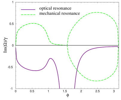
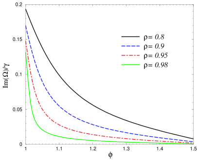
FIG. 8.: The growth of instabilities for highly reflecting SR mirrors. In the left panel we plot the imaginary part of the resonant frequencies, obtained solving Eq. (102), versus the SR detuning phase $\phi$, for $\rho=0.9$ and $I_{0}=I_{\rm SQL}\simeq 10^{4}\,{\rm W}$. On the right panel we blow up the plot shown in the left panel for the detuning region ${\cal D}=\{\phi:\arctan[(4I_{0}/I_{\rm SQL})^{1/3}]<\phi<\pi/2\}$, fixing $\rho=0.8,0.9,0.95,0.98$ and $I_{0}=I_{\rm SQL}\simeq 10^{4}\,{\rm W}$. This range of physical parameters corresponds to interesting LIGO-II noise curves [13, 14].

In Ref. [14], by analyzing the case of very highly reflecting SR mirrors ($\rho\rightarrow 1$) the authors found interesting noise curves for the detuning range ${\cal D}=\{\phi:\arctan[(4I_{0}/I_{\rm SQL})^{1/3}]<\phi<\pi/2\}$ [see Sec. IV A and, in particular, Eq. (4.4) of Ref. [14]]. In the right panel of Fig. 8, we blow up the left panel around this region ${\cal D}$ and plot various curves obtained by varying the SR reflectivity $\rho=0.8,0.9,0.95$ and $0.98$. We observe that, for this parameter set, the largest growth rate is $\sim\!0.2\gamma\sim\!124\,{\rm s}^{-1}$, corresponding to an e-folding time of $8$ ms, which is five times larger than the arm-cavity storage time.

Finally, we notice that the kind of instability we have found in SR interferometers has an origin similar to the dynamical instability induced in a detuned Fabry-Perot cavity by the radiation-pressure force acting on the mirrors [36, 33, 34].

V Control systems for signal recycled interferometers

In this section we discuss how to suppress the instabilities present in SR interferometers by a suitable servo system. Since the control system must sense the mirror motion inside the observation band and act on (usually damp) it, there is an issue to worry about: If the dynamics is changed by the control system, it is not clear a priori whether the resonant dips (or at least the mechanical one which corresponds to the unstable resonance), which characterize the noise curves in the uncontrolled SR interferometer [13, 14], will survive. In the following we shall show the existence of control systems that suppress the instability without altering the noise curves of uncontrolled interferometers, thereby relieving ourselves from the above worry.

A Generic feed-back control systems: changing the dynamics without affecting the noise

We shall identify a broad category of control systems for which, if the instability can be suppressed, the noise curves are not altered. We suppose that the output signal $\widehat{Z}$ is sent through a linear filter $K_{\cal C}$ and then applied to the antisymmetric mode of the arm-cavity mirrors (see the schematic drawing in Fig. 9). This operation corresponds to modifying the Hamiltonian (7) into the form

$$\widehat{H}=[(\widehat{H}_{\cal P}-\widehat{x}\,G)+\widehat{H}_{\cal D}]-\widehat{x}\,\widehat{F}-\widehat{x}\,\widehat{\cal C}\,,$$ (107)

where $\widehat{\cal C}$ is a detector observable whose free Heisenberg operator (evolving under $H_{\cal D}$) at time $t$ is given, as required by causality, by an integration over $t^{\prime}<t$,

$$\widehat{\cal C}^{(0)}(t)=\int_{-\infty}^{t}dt^{\prime}\,K_{\cal C}(t-t^{\prime})\,\widehat{Z}^{(0)}(t^{\prime})\,.$$ (108)

Physically the filter kernel $K_{\cal C}(\tau)$ should be a function defined for $\tau>0$ and should decay to zero when $\tau\rightarrow+\infty$. However, in order to apply Fourier analysis, we can extend its definition to $\tau<0$ by imposing $K_{\cal C}(\tau<0)\equiv 0$, thereby obtaining

$$\widehat{\cal C}^{(0)}(t)=\int_{-\infty}^{+\infty}dt^{\prime}\,K_{\cal C}(t-t^{\prime})\,\widehat{Z}^{(0)}(t^{\prime}).$$ (109)

Therefore, in the Fourier domain we have

$$\widehat{\cal C}^{(0)}(\Omega)=K_{\cal C}(\Omega)\widehat{Z}^{(0)}(\Omega),$$ (110)

where $K_{\cal C}(\Omega)$ is the Fourier transform of $K_{\cal C}(\tau)$. It is straightforward to show that the two time-domain properties $K_{\cal C}(\tau<0)=0$ and $K_{\cal C}(\tau\rightarrow+\infty)\rightarrow 0$ correspond in the Fourier domain to the requirement that $K_{\cal C}(\Omega)$ have poles only in the lower-half $\Omega$ plane.

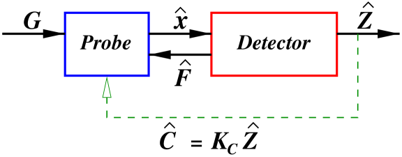
FIG. 9.: Scheme of the control system introduced to quench the instabilities present in a SR interferometer. The output $\widehat{Z}$, which contains the GW signal and the quantum noise, is sent through a linear filter with output $\widehat{\cal C}=K_{\cal C}\,\widehat{Z}$, and is then fed back onto the probe, i.e. the antisymmetric mode of motion of the four arm-cavity mirrors.

Working in the Fourier domain and assuming that the readout scheme is homodyne detection with detection phase $\zeta={\rm const}$, we derive a set of equations of motion similar to Eqs. (86)–(88),

$$\widehat{Z}_{\zeta}^{(1)}(\Omega) = \widehat{Z}_{\zeta}^{(0)}(\Omega)+\left[R_{Z_{\zeta}F}(\Omega)+R_{Z_{\zeta}{\cal C}_{\zeta}}(\Omega)\right]\,\widehat{x}^{(1)}(\Omega)\,,$$ (111)

$$\widehat{F}^{(1)}(\Omega) = \widehat{F}^{(0)}(\Omega)+\left[R_{FF}(\Omega)+R_{FC_{\zeta}}(\Omega)\right]\,\widehat{x}^{(1)}(\Omega)\,,$$ (112)

$$\widehat{x}^{(1)}(\Omega) = R_{xx}(\Omega)\,[G(\Omega)+\widehat{F}^{(1)}(\Omega)+\widehat{\cal C}_{\zeta}^{(1)}(\Omega)]\,,$$ (113)

$$\widehat{\cal C}_{\zeta}^{(1)}(\Omega) = \widehat{\cal C}_{\zeta}^{(0)}(\Omega)+\left[R_{{\cal C}_{\zeta}F}(\Omega)+R_{{\cal C}_{\zeta}{\cal C}_{\zeta}}(\Omega)\right]\,\widehat{x}^{(1)}(\Omega)\,.$$ (114)

Each of Eqs. (111), (112) and (114) has two response terms due to the two coupling terms between the probe and the detector in the total Hamiltonian (107). However, some of the responses are actually zero. In particular, inserting Eq. (108) into $[\widehat{F}^{(0)}(t),\widehat{\cal C}_{\zeta}^{(0)}(t^{\prime})]$ and using the fact that $[\widehat{F}^{(0)}(t),\widehat{Z}_{\zeta}^{(0)}(t^{\prime})]=0$ for $t>t^{\prime}$ [see Eq. (37)], we find $R_{FC_{\zeta}}(\Omega)=0$. Combining Eq. (108) with the fact that $[\widehat{Z}_{\zeta}^{(0)}(t),\widehat{Z}_{\zeta}^{(0)}(t^{\prime})]=0$ for all $t,\,t^{\prime}$ [see Eq. (37)], we have $R_{Z_{\zeta}{\cal C}_{\zeta}}(\Omega)=0=R_{{\cal C}_{\zeta}{\cal C}_{\zeta}}(\Omega)$. Moreover, the fact that $K_{\cal C}(t-t^{\prime})=0=C_{Z^{(0)}F^{(0)}}(t,t^{\prime})$ for $t<t^{\prime}$ gives the equality $R_{{\cal C}_{\zeta}F}(\Omega)=K_{\cal C}(\Omega)\,R_{Z_{\zeta}F}(\Omega)$. Imposing these conditions, we deduce a simplified set of equations of motion:

$$\widehat{Z}_{\zeta}^{(1)}(\Omega) = \widehat{Z}_{\zeta}^{(0)}(\Omega)+R_{Z_{\zeta}F}(\Omega)\,\widehat{x}^{(1)}(\Omega)\,,$$ (115)

$$\widehat{F}^{(1)}(\Omega) = \widehat{F}^{(0)}(\Omega)+R_{FF}(\Omega)\,\widehat{x}^{(1)}(\Omega)\,,$$ (116)

$$\widehat{x}^{(1)}(\Omega) = R_{xx}(\Omega)\,[G(\Omega)+\widehat{F}^{(1)}(\Omega)+\widehat{\cal C}_{\zeta}^{(1)}(\Omega)]\,,$$ (117)

$$\widehat{\cal C}_{\zeta}^{(1)}(\Omega) = K_{\cal C}(\Omega)\,\widehat{Z}^{(1)}(\Omega)\,.$$ (118)

Solving Eqs. (115)–(118), we obtain

$$\widehat{x}^{(1)}(\Omega)=\frac{R_{xx}}{1-R_{xx}\,\left(R_{FF}+R_{Z_{\zeta}F}\,K_{\cal C}\right)}\left[G(\Omega)+\widehat{F}^{(0)}(\Omega)+K_{\cal C}(\Omega)\,\widehat{Z}_{\zeta}^{(0)}(\Omega)\right]\,,$$ (119)

$$\widehat{Z}_{\zeta}^{(1)}(\Omega)=\frac{1-R_{xx}\,R_{FF}}{1-R_{xx}\,\left(R_{FF}+R_{Z_{\zeta}F}\,K_{\cal C}\right)}\left\{\widehat{Z}_{\zeta}^{(0)}(\Omega)+\frac{R_{Z_{\zeta}F}\,R_{xx}}{1-R_{xx}\,R_{FF}}\,\left[G(\Omega)+\widehat{F}^{(0)}(\Omega)\right]\right\}\,,$$ (120)

$$\widehat{F}^{(1)}(\Omega)=\frac{1-K_{\cal C}\,R_{xx}\,R_{Z_{\zeta}F}}{1-R_{xx}\,\left(R_{FF}+R_{Z_{\zeta}F}\,K_{\cal C}\right)}\left\{\widehat{F}^{(0)}(\Omega)+\frac{R_{FF}\,R_{xx}}{{1-K_{\cal C}\,R_{xx}\,R_{Z_{\zeta}F}}}\,\left[G(\Omega)+K_{\cal C}\,\widehat{Z}^{(0)}(\Omega)\right]\right\}\,.$$ (121)

From the above equations (119)–(121), we infer that the stability condition for the controlled system is determined by the positions of the roots of $[1-R_{xx}(R_{FF}+R_{Z_{\zeta}F}K_{\cal C})]$. Therefore, by choosing the filter kernel $K_{\cal C}$ appropriately, it may be possible that all the roots have negative imaginary part, in which case the system will be stable.

Before working out a specific control kernel $K_{\cal C}$ that suppresses the instability, let us notice that different choices of $K_{\cal C}$ give outputs (120) that differ only by an overall frequency-dependent normalization factor. This factor does not influence the interferometer’s noise, since from Eq. (120) we can see that the relative magnitudes of the signal (term proportional to $G$) and the noise (terms proportional to $\widehat{Z}^{(0)}_{\zeta}$ and $\widehat{F}^{(0)}$) depend only on the quantities inside the brackets $\{\quad\}$ and not on the factor multiplying the bracket [see Ref. [14] for a detailed discussion of the noise spectral density]. Therefore if this control system can suppress the instability, the resulting well-behaved controlled SR interferometer will have the same noise as evaluated in Refs. [13, 14] for the uncontrolled SR interferometer. This important fact can be easily understood by observing that, because the whole output (the GW signal $h$ and the noise $N$) is fed back onto the arm-cavity mirrors, $h$ and $N$ are suppressed in the same way by the control system, and thus their relative magnitude at any frequency $\Omega$ is the same as if the SR interferometer had been uncontrolled.

B An example of a servo system: effective damping of the test-mass

Physically, it is quite intuitive to think of the feed-back system as a system that effectively “damps” the test-mass motion. When the control system is present, the equation of motion for the antisymmetric mode can be obtained from Eqs. (117), (115) and (118). It reads [as compared to Eq. (88)]:

$$\widehat{x}^{(1)}(\Omega)=\frac{R_{xx}}{1-K_{\cal C}\,R_{xx}\,R_{Z_{\zeta}F}}\left[G(\Omega)+\widehat{F}^{(1)}(\Omega)+K_{\cal C}\,\widehat{Z}_{\zeta}^{(0)}(\Omega)\right]\,.$$ (122)

Denoting by ${R}^{\cal C}_{xx}$ the response of $\widehat{x}^{(1)}$ to $G$ and $\widehat{F}^{(1)}$ when the servo system is present, i.e.

$${R}^{\cal C}_{xx}=\frac{R_{xx}}{1-K_{\cal C}\,R_{xx}\,R_{Z_{\zeta}F}}\,,$$ (123)

we can rewrite the overall normalization factor which appears in Eqs. (119)–(121) as

$$\frac{1}{1-R_{xx}\,\left(R_{FF}+R_{Z_{\zeta}F}\,K_{\cal C}\right)}=\frac{R^{\cal C}_{xx}}{R_{xx}}\,\frac{1}{1-R^{\cal C}_{xx}\,R_{FF}}\,.$$ (124)

A sufficient condition for stability is that both ${R^{\cal C}_{xx}}/{R_{xx}}$ and ${1}/({1-R^{\cal C}_{xx}R_{FF}})$ have poles only in the lower-half complex plane. [Note that when the servo system is present $R^{\cal C}_{xx}$ replaces $R_{xx}$ in the stability condition of the system, see Sec. II B, Eqs. (21)–(23) and discussions after them.]

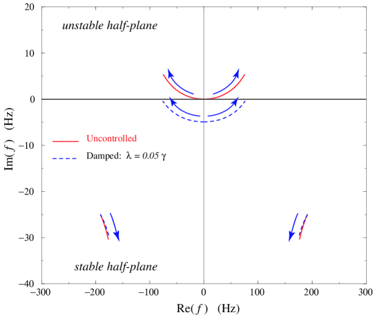
FIG. 10.: Effective damping due to a servo system with control kernel given by Eq. (127). We have fixed: $\lambda=0.05\,\gamma$, $\rho=0.9$, $\phi=\pi/2-0.47$ and $I_{0}$ from $\sim 0$ up to $I_{\rm SQL}\simeq 10^{4}\,{\rm W}$. The arrows indicate the directions of increasing light power $I_{0}$. The originally unstable mechanical resonance (solid line) is pushed downward in the complex $\Omega$-plane, and stabilized (dashed line). The figure also shows the effect of the control system on the stable optical resonances.

We have found it natural to choose for $R^{\cal C}_{xx}(\Omega)$ the susceptibility of a damped oscillator (with effective mass $m/4$), having both poles in the lower-half $\Omega$ plane at $\Omega=-i\lambda$, i.e. 

$${R}^{\cal C}_{xx}(\Omega)=-\frac{4}{m}\,\frac{1}{(\Omega+i\lambda)^{2}}\,,$$ (126)

with $\lambda$ a real parameter. This choice automatically ensures that ${R^{\cal C}_{xx}}/{R_{xx}}$ has poles only in the lower-half complex plane. Moreover, by choosing $\lambda$ appropriately we can effectively push the roots of $(1-{R}^{\cal C}_{xx}\,R_{FF})$ in Eq. (124) to the lower-half $\Omega$ plane, as shown in Fig. 10 for $\rho=0.9$, $\phi=\pi/2-0.47$, $\lambda=0.05\,\gamma$ and $I_{0}$ from $\sim 0$ up to $I_{\rm SQL}$.

However, we also need to check that $K_{\cal C}(\Omega)$ has poles only in the lower-half $\Omega$ plane. Using Eqs. (123), (126) we obtain the following explicit expression for the kernel:

$$K_{\cal C}(\Omega) = \frac{1}{R_{Z_{\zeta}F}}\left(\frac{1}{R_{xx}}-\frac{1}{R^{\cal C}_{xx}}\right)$$ (127)

$$= \frac{m\lambda}{2\,\tau}\sqrt{\frac{\hbar L^{2}}{2I_{0}\omega_{0}}}\left(\Omega+\frac{i\lambda}{2}\right)\frac{(1+2\rho\cos 2\phi+\rho^{2})(\Omega-\Omega_{-})(\Omega-\Omega_{+})}{(\Omega+i\gamma)\cos(\phi+\zeta)+\rho(\Omega-i\gamma)\cos(\phi-\zeta)}\,.$$ (128)

For $\zeta=0$ or $\zeta=\pi/2$, i.e. when either of the two quadratures $\widehat{b}_{1}$ or $\widehat{b}_{2}$ is measured, the control kernel (127) indeed has poles only in the lower-half complex plane. More generally, we have shown that if $0<\phi<\pi/2$, the control kernel (127) has poles in the lower-half complex plane for all $\pi/2\leq\zeta\leq\pi$, regardless of the value of $\rho$, but it may become unphysical in the region $0<\zeta<\pi/2$. However, for the unphysical values of $\zeta$ there are various feasible ways out. For example, we could change $R^{\cal C}_{xx}$ by replacing $m$ in Eq. (126) with a slightly smaller quantity $m_{\cal C}$. In this case

$$\left(\frac{1}{R_{xx}}-\frac{1}{R^{\cal C}_{xx}}\right)=-\frac{m}{4}\,\left[\Omega\,\left(1-\sqrt{\frac{m_{\cal C}}{m}}\right)-i\lambda\,\sqrt{\frac{m_{\cal C}}{m}}\,\right]\,\left[\Omega\,\left(1+\sqrt{\frac{m_{\cal C}}{m}}\right)+i\lambda\,\sqrt{\frac{m_{\cal C}}{m}}\,\right]\,.$$ (129)

By choosing $m_{\cal C}$ appropriately, we can use the first factor in Eq. (129), which has a root in the upper-half complex plane, to cancel the bad pole coming from $R_{Z_{\zeta}F}$ in Eq. (127), so that $K_{\cal C}$ will have poles only in the lower-half complex plane. Finally, we must adjust $\lambda$ so that the effective damping suppress the instability.

Of course, the servo electronics employed to implement the control system will inevitably introduce some noise into the interferometer. In our investigation we have not modelled this noise. However, LIGO experimentalists have seen no fundamental noise limit in implementing control kernels of the kind we discussed, and deem it technically possible to suppress any contribution coming from the electronics to within 10% of the total predicted quantum noise [37, 38]. This issue deserves a more careful study and it will be tackled elsewhere [39].

In this paper we have restricted ourselves to the readout scheme of frequency independent homodyne detection, in which only one (frequency independent) quadrature $b_{\zeta}$ is measured. The issue of control-system design when other readout schemes are present, e.g., the so-called radio-frequency modulation-demodulation design, is currently under investigation [39].

Finally, for simplicity we have limited our discussion to lossless SR interferometers. When optical losses are taken into account, we have found that the instability problem is still present [14] and we have checked that those instabilities can be cured by the same type of control system as was discussed above for lossless SR interferometers.

VI Conclusions

Using the formalism of linear quantum-measurement theory, extended by Braginsky and Khalili [21] to GW detectors, we have described the optical-mechanical dynamics of SR interferometers such as LIGO-II [3]. This analysis has allowed us to work out various significant features of such interferometers, which previous investigations [4, 5, 6, 7, 8] could not reveal.

We have found that when the (carrier) laser frequency is detuned in the SR cavity, the arm-cavity mirrors are not only perturbed by a random fluctuating force but are also subject to a linear restoring force with a specific frequency-dependent rigidity. This phenomenon is not unique to SR interferometers; it is a generic feature of detuned cavities [36, 20, 33, 34] and was originally used by Braginsky, Khalili and colleagues in designing the “optical bar” GW detectors [20].

Our analysis has revealed that, for SR interferometers, the dynamics of the whole optical-mechanical system, composed of the arm-cavity mirrors and the optical field, resembles that of a free test mass (mirror motion) connected to a massive spring (optical fields). When the test mass and the spring are not connected (e.g., for very low laser power) they have their own eigenmodes, namely the uniform translation mode for the free test mass (free antisymmetric mode), and the longitudinal-wave mode for the spring (decoupled SR optical resonance). However, as soon as the free test mass is connected to the massive spring (e.g, for LIGO-II laser power), the two free modes get shifted in frequency, so the entire coupled system can resonate at two pairs of finite frequencies (coupled mechanical and optical resonances). From this point of view a SR interferometer behaves like an “optical spring” detector. For LIGO-II parameters, both resonant frequencies can lie in the observation band $10\,{\rm Hz}<f<10\,{\rm kHz}$ and they are responsible for the beating of the SQL in SR interferometers  [13, 14].

The formalism used in the present paper has allowed us to analyze in more detail the features of the instabilities in SR interferometers, pointed out in Refs. [13, 14]. Most importantly, we have shown the possibility of using a feed-back control system to cure such instabilities without compromising the performance of the interferometer. However, before any practical implementation, a much more careful and precise study should be carried out, including various readout schemes [39].

Finally, the general discussion based on the Braginsky-Khalili force-susceptibility formalism, given in the first part of this paper (Sec. II), and the application to a specific type of GW interferometer, the LIGO-II SR interferometer, given in the second part of it (Secs. III–V), may provide, along with Refs. [12, 14], a framework for future investigations of quantum noise in advanced, more complex, optical configurations.

A Basic properties of linear systems

In this Appendix, to clarify the formalism used in Sec. II, we summarize some well-known basic properties of linear systems linearly coupled to each other or to external classical forces. Much of this material can be found in Sakurai [40], and for its application to quantum-measurement processes in Braginsky and Khalili [21] and Caves et al. [25].

Definition 1 (Linear systems)

Any system whose Hamiltonian is at most quadratic in its canonical coordinates and momenta is a linear system.

Definition 2 (Linear observables)

Any linear combination (either time dependent or time independent) of the canonical coordinates and momenta of a linear system, plus a possible complex number (C-number), is a linear observable of the system.

Denoting all the canonical coordinates and momenta by $\widehat{{\cal C}}_{i}$ with $i=1,2,\cdots$, the Hamiltonian of a linear system can be written as

$$\widehat{H}(t)=\sum_{i,j}L^{ij}_{2}(t)\,\widehat{\cal C}_{i}\,\widehat{\cal C}_{j}+\sum_{i}L^{i}_{1}(t)\,\widehat{{\cal C}}_{i}+L_{0}(t)\,,$$ (A1)

where $L^{ij}_{2}(t)$ is symmetric in $i$ and $j$. The equations of motion of the canonical observables in the Heisenberg picture read [we use the fact that $\widehat{\cal C}_{jH}$ does not depend explicitly on time]:

$$i\hbar\frac{d}{dt}\widehat{\cal C}_{jH}(t) = \left[\widehat{\cal C}_{jH}(t),\widehat{H}_{H}(t)\right]\,,$$ (A2)

$$= \widehat{U}^{\dagger}(-\infty,t)\,\left[\widehat{\cal C}_{jS},\widehat{H}_{S}(t)\right]\,\widehat{U}(-\infty,t)\,,$$ (A3)

$$= \widehat{U}^{\dagger}(-\infty,t)\left[\sum_{l,m}2\,L_{2}^{lm}(t)\,C_{jl}\,\widehat{\cal C}_{mS}+\sum_{l}L_{1}^{l}(t)\,C_{jl}\right]\widehat{U}(-\infty,t)\,,$$ (A4)

$$= \sum_{l,m}2\,L_{2}^{lm}(t)\,C_{jl}\,\widehat{\cal C}_{mH}(t)+\sum_{l}L_{1}^{l}(t)\,d_{jl}\,.$$ (A5)

Here the subscripts $S$ and $H$ stand for Schrödinger and Heisenberg pictures respectively, $C_{jl}\equiv[\widehat{\cal C}_{jS},\widehat{\cal C}_{lS}]$ is the commutator between the canonical operators, which is a C-number, and $\widehat{U}(-\infty,t)$ is the time-evolution operator which satisfies the Schrödinger equation

$$i\hbar\frac{d}{dt}\widehat{U}(-\infty,t)=\widehat{H}_{S}\,\widehat{U}(-\infty,t)$$ (A6)

with initial condition $\widehat{U}(-\infty,-\infty)=1.$ The solution to Eq. (A2) is of the form

$$\widehat{\cal C}_{jH}(t)=\sum_{k}\alpha_{jk}(t)\,\widehat{\cal C}_{kH}(-\infty)+\beta_{j}(t)=\sum_{k}\alpha_{jk}(t)\,\widehat{\cal C}_{kS}+\beta_{j}(t)\,,$$ (A7)

where $\alpha_{jk}(t)$ and $\beta_{j}(t)$ are time dependent C-numbers.

For any linear observable $A$ it follows from linearity that $\widehat{A}_{H}(t)=\sum_{j}a_{j}(t)\,\widehat{\cal C}_{jH}(t)+b(t)$, which, along with Eq. (A7), leads to:

$$\widehat{A}_{H}(t)=\sum_{j}a_{j}(t)\,\widehat{\cal C}_{jH}(t)+b(t)=\sum_{j,k}a_{j}(t)\,\alpha_{jk}(t)\,\widehat{\cal C}_{kS}+\sum_{j}a_{j}(t)\beta_{j}(t)+b(t)\,.$$ (A8)

This provides the following theorem:

Theorem 1

At any time the operator of a linear observable in the Heisenberg picture can always be written as a linear combination of operators of the (time-independent) canonical variables in the Schrödinger picture plus a possible C-number.

Applying the above theorem to any two linear observables $A$ and $B$, recalling that $C_{jk}\equiv[\widehat{\cal C}_{jS},\widehat{\cal C}_{kS}]$ is a C-number and the commutator between a C-number and any operator is zero, we find

$$\left[\widehat{A}_{H}(t),\widehat{B}_{H}(t^{\prime})\right]=\sum_{j,k}\gamma_{j}^{A}(t)\,\gamma^{B}_{k}(t^{\prime})\,C_{jk}\,,$$ (A9)

which is a C-number. Therefore, the following theorem holds:

Theorem 2

In the Heisenberg picture, the commutator of the operators of any two linear observables at two times is a C-number.

We are interested in the evolution of a linear system subject to a classical external linear force or linearly coupled to another independent linear system. A force-susceptibility kind of formulation can be introduced in these cases (as is done by Braginsky and Khalili, see Sec. 6.4 of Ref. [21]). We shall describe the system using a perturbative approach. Thus we write the total Hamiltonian in the Schrödinger picture as $\widehat{H}_{S}=\widehat{H}_{0S}+\widehat{V}_{S}(t)$, where $\widehat{V}_{S}(t)$ is treated as a perturbation with respect to the zeroth order Hamiltonian $\widehat{H}_{0S}$. It is generally convenient to introduce the so-called Interaction picture (see, e.g., Sections 5.5 and 5.6 of Ref. [40]), in which the evolution operator $\widehat{U}_{I}$ is defined by the relation $\widehat{U}(-\infty,t)\equiv\widehat{U}_{0}(-\infty,t)\,\widehat{U}_{I}(-\infty,t)$, where $\widehat{U}_{0}(-\infty,t)$ is the evolution operator associated with $\widehat{H}_{0S}$ and $\widehat{U}$ is defined by Eq. (A6). Then, $\widehat{U}_{I}(-\infty,t)$ satisfies the equations

$$i\hbar\frac{d}{dt}\widehat{U}_{I}(-\infty,t)=\widehat{V}_{I}(t)\,\widehat{U}_{I}(-\infty,t)\,,\quad\quad\widehat{U}_{I}(-\infty,-\infty)=1\,,$$ (A10)

with $\widehat{V}_{I}(t)\equiv\widehat{U}^{\dagger}_{0}(-\infty,t)\,\widehat{V}_{S}(t)\,\widehat{U}_{0}(-\infty,t)$. The solution of Eq. (A10) can be written as a perturbative expansion,

$$\widehat{U}_{I}(-\infty,t) = 1+\frac{1}{i\hbar}\int_{-\infty}^{t}dt_{1}\widehat{V}_{I}(t_{1})+\left(\frac{1}{i\hbar}\right)^{2}\int_{-\infty}^{t}dt_{1}\int_{-\infty}^{t_{1}}dt_{2}\widehat{V}_{I}(t_{1})\widehat{V}_{I}(t_{2})+\cdots\,,$$ (A11)

$$= \sum_{n=0}^{\infty}\frac{1}{n!}\left(\frac{1}{i\hbar}\right)^{n}T\left\{\left[\int_{-\infty}^{t}dt_{1}\widehat{V}_{I}(t_{1})\right]^{n}\right\}\,,$$ (A12)

where $T$ denotes the time-ordered product [41]. The Heisenberg operator associated with any observable $A$, evolving under the full Hamiltonian $\widehat{H}$, is linked to the corresponding Heisenberg operator evolving under the Hamiltonian $\widehat{H}_{0}$ by the relation $\widehat{A}_{H}(t)=\widehat{U}_{I}^{\dagger}(-\infty,t)\widehat{A}_{H}^{(0)}(t)\widehat{U}_{I}(-\infty,t)$, where the superscript $(0)$ on the observable $A$ denotes that the evolution is due to $\widehat{H}_{0}$. Inserting Eq. (A12) into the above equation, we get

$$\widehat{A}_{H}(t)=\widehat{A}_{H}^{(0)}(t)+\frac{i}{\hbar}\int_{-\infty}^{t}dt_{1}\left[\widehat{V}_{I}(t_{1}),\widehat{A}^{(0)}_{H}(t)\right]+\left(\frac{i}{\hbar}\right)^{2}\int_{-\infty}^{t}dt_{1}\int_{-\infty}^{t_{1}}dt_{2}\left[\widehat{V}_{I}(t_{2}),\left[\widehat{V}_{I}(t_{1}),\widehat{A}^{(0)}_{H}(t)\right]\right]$$ (A13)

$$+\cdots+\left(\frac{i}{\hbar}\right)^{n}\int_{-\infty}^{t}dt_{1}\int_{-\infty}^{t_{1}}dt_{2}\cdots\int_{-\infty}^{t_{n-1}}dt_{n}\left[\widehat{V}_{I}(t_{n}),\left[\cdots,\left[\widehat{V}_{I}(t_{2}),\left[\widehat{V}_{I}(t_{1}),\widehat{A}^{(0)}_{H}(t)\right]\right]\cdots\right]\right]+\cdots\,.$$ (A14)

For a linear system subject to an external classical linear force $G(t)$, the interaction term is $\widehat{V}_{I}(t)=-\widehat{x}_{H}^{(0)}G(t)$. Plugging this expression into Eq. (A14) and using Theorem 2, it is straightforward to deduce that the second and all higher order terms in Eq. (A14) vanish and the first order perturbation gives the exact solution. Hence, we obtain the following theorem:

Theorem 3

Consider a linear system subject to a classical generalized force $G(t)$, whose Hamiltonian is given by $\widehat{H}=\widehat{H}_{0}-\widehat{x}\,G(t)$, where $\widehat{x}$ is a linear observable. Then, for any linear observable $\widehat{A}$, the Heisenberg operator $\widehat{A}_{H}(t)$ can be written as the sum of its free-evolution part, $\widehat{A}^{(0)}_{H}(t)$, plus a term which is due to the presence of the external force, i.e.

$$\widehat{A}_{H}(t)={\widehat{A}^{(0)}}_{H}(t)+\frac{i}{\hbar}\int^{t}_{-\infty}dt^{\prime}\,C_{Ax}(t,t^{\prime})\,G(t^{\prime})\,,$$ (A15)

where $C_{Ax}(t,t^{\prime})$ is a C-number, called the (time-domain) susceptibility, given explicitly by

$$C_{Ax}(t,t^{\prime})\equiv[\widehat{A}_{H}^{(0)}(t),\widehat{x}_{H}^{(0)}(t^{\prime})]\,.$$ (A16)

Let us now suppose that we have two independent linear systems ${\cal P}$ (e.g., the probe) and ${\cal D}$ (e.g., the detector), which by definition are described by two different Hilbert spaces $\cal{H}_{\cal P}$ and $\cal{H}_{\cal D}$. We introduce the Hilbert space ${\cal H}={\cal H}_{\cal P}\otimes{\cal H}_{\cal D}$ and define for any operator $\widehat{x}$ of the system ${\cal P}$ the corresponding operator acting on ${\cal H}$ as $\widehat{x}\otimes\widehat{1}$, while for any operator $\widehat{F}$ of the system ${\cal D}$ we introduce the operator $\widehat{1}\otimes\widehat{F}$ which acts on ${\cal H}$. Henceforth, we shall limit ourselves to interaction terms $V$, in the total Hamiltonian $\widehat{H}=\widehat{H}_{\cal P}+\widehat{H}_{\cal D}+\widehat{V}$, of the form: $\widehat{V}=-\widehat{x}\otimes\widehat{F}$, with $\widehat{x}$ and $\widehat{F}$ acting on ${\cal P}$ and ${\cal D}$, respectively. Using Eq. (A14) with $\widehat{V}_{I}(t)=-\widehat{x}_{H}^{(0)}(t)\widehat{F}_{H}^{(0)}(t)$, noticing that (i) the zeroth order Heisenberg operators of two observables living in different Hilbert spaces commute and (ii) the zeroth order Heisenberg operators of two linear observables living in the same Hilbert space have a C-number commutator, we derive the following theorem:

Theorem 4

Consider two independent linear systems ${\cal P}$ and ${\cal D}$, and two linear observables, $\widehat{x}$ of ${\cal P}$ and $\widehat{F}$ of ${\cal D}$. Suppose that the two systems are coupled by a term $-\widehat{x}\otimes\widehat{F}$, i.e. the Hamiltonian of the composite system ${\cal P}$ + ${\cal D}$ reads $\widehat{H}=\widehat{H}_{\cal P}+\widehat{H}_{\cal D}-\widehat{x}\otimes\widehat{F}.$ Then, for any linear observable $\widehat{A}$ of the system ${\cal P}$ and $\widehat{B}$ of the system ${\cal D}$, their full Heisenberg evolutions are given by:

$$\widehat{A}_{H}(t)=\widehat{A}^{(0)}_{H}(t)+\frac{i}{\hbar}\,\int^{t}_{-\infty}dt^{\prime}C_{Ax}(t,t^{\prime})\,\widehat{F}_{H}(t^{\prime})\,,\quad\quad\widehat{B}_{H}(t)=\widehat{B}^{(0)}_{H}(t)+\frac{i}{\hbar}\,\int^{t}_{-\infty}dt^{\prime}C_{BF}(t,t^{\prime})\,\widehat{x}_{H}(t^{\prime})\,,$$ (A17)

where $\widehat{A}^{(0)}_{H}$ and $\widehat{B}^{(0)}_{H}$ stand for the free Heisenberg evolutions, and the susceptibilities are defined by

$$C_{Ax}(t,t^{\prime})\equiv[\widehat{A}_{H}^{(0)}(t),\widehat{x}_{H}^{(0)}(t^{\prime})]\,,\quad\quad C_{BF}(t,t^{\prime})\equiv[\widehat{B}_{H}^{(0)}(t),\widehat{F}_{H}^{(0)}(t^{\prime})]\,.$$ (A18)

In the case where the zeroth order Hamiltonian is time independent, it is easy and convenient to express the above formalism in the Fourier domain. We first notice that for a time independent $\widehat{H}_{0}$, $\widehat{U}_{0}(t,t+\tau)=e^{-i\widehat{H}_{0}\tau/\hbar}$ and for any two linear observables $\widehat{A}_{1}$ and $\widehat{A}_{2}$ we have $C_{A_{1}A_{2}}(t+\tau,t^{\prime}+\tau)=C_{A_{1}A_{2}}(t,t^{\prime})$, i.e. $C_{A_{1}A_{2}}(t,t^{\prime})$ depends only on $t-t^{\prime}$. Defining the Fourier transform of any observable $\widehat{A}(t)$ as

$$\widehat{A}(\Omega)\equiv\int_{-\infty}^{+\infty}dt\,e^{i\Omega t}\,\widehat{A}(t)\,,$$ (A19)

Eq. (A15) becomes $\widehat{A}_{H}(\Omega)=\widehat{A}^{(0)}_{H}(\Omega)+R_{Ax}(\Omega)\,G(\Omega)$ while Eq. (A17) can be recast in the form

$$\widehat{A}_{H}(\Omega)=\widehat{A}^{(0)}_{H}(\Omega)+R_{Ax}(\Omega)\,\widehat{F}_{H}(\Omega)\,,\quad\quad\widehat{B}_{H}(\Omega)=\widehat{B}^{(0)}_{H}(\Omega)+R_{BF}(\Omega)\,\widehat{x}_{H}(\Omega)\,,$$ (A20)

where $R_{AB}(\Omega)$ is the susceptibility in the Fourier-domain, given by

$$R_{AB}(\Omega)=\frac{i}{\hbar}\int_{-\infty}^{+\infty}d\tau\,e^{i\Omega\tau}\,\Theta(\tau)C_{AB}(0,-\tau)=\frac{i}{\hbar}\int_{0}^{+\infty}d\tau\,e^{i\Omega\tau}\,C_{AB}(0,-\tau)\,,$$ (A21)

with $\Theta(\tau)$ the step function. For future reference, let us point out two properties which $R_{AB}(\Omega)$ satisfies and that we use repeatedly in Sec. II:

$$R^{*}_{AB}(\Omega)=R_{AB}(-\Omega)\,,\quad\quad\left[\widehat{A}^{(0)}_{H}(\Omega_{1}),\widehat{B}^{(0)}_{H}(\Omega_{2})\right]=-2\pi i\hbar\delta(\Omega_{1}+\Omega_{2})\left[R_{AB}(\Omega_{1})-R_{BA}(\Omega_{2})\right]\,.$$ (A22)

To deduce the first identity in Eq. (A22), we consider the complex (Hermitian) conjugate of Eq. (A21) and use the Hermiticy of $\widehat{A}^{(0)}_{H}(t)$ and $\widehat{B}^{(0)}_{H}(t)$. For the second identity in Eq. (A22), we take the double Fourier transform of $[\widehat{A}^{(0)}_{H}(t_{1}),\widehat{B}^{(0)}_{H}(t_{2})]$ with respect to $t_{1}$ and $t_{2}$, and then using Eq. (A21) we find that the region corresponding to $t_{1}>t_{2}$ in the double integral yields the $R_{AB}$ term of Eq. (A22), while the region corresponding to $t_{1}<t_{2}$ gives the $R_{BA}$ term.

REFERENCES

- [1] A. Abramovici, W.E. Althouse, R.W.P. Drever, Y. Gursel, S. Kawamura, F.J. Raab, D. Shoemaker, L. Sievers, R.E. Spero, K.S. Thorne, R.E. Vogt, R. Weiss, S.E. Whitcomb, and M.E. Zucker, Science 256, 325 (1992); B. Caron et al., Class. Quantum Grav. 14, 1461 (1997); H. Lück et al., Class. Quantum Grav. 14, 1471 (1997); M. Ando et al., “Stable operation of a 300-m laser interferometer with sufficient sensitivity to detect gravitational-wave events within our galaxy,” astro-ph/0105473.
- [2] See, e.g., A. Abramovici et al. in Ref. [1]; K.S. Thorne, in Proceedings of the Snowmass 95 Summer Study on Particle and Nuclear Astrophysics and Cosmology, eds. E.W. Kolb and R. Peccei (World Scientific, Singapore, 1995), p 398, gr-qc/9506085; K.S. Thorne, “The scientific case for mature LIGO interferometers,” (LIGO Document Number P000024-00-R, www.ligo.caltech.edu/docs/P/P000024-00.pdf).
- [3] E. Gustafson, D. Shoemaker, K.A. Strain and R. Weiss, “LSC White paper on detector research and development,” (LIGO Document Number T990080-00-D, www.ligo.caltech.edu/docs/T/T990080-00.pdf).
- [4] R.W.P. Drever, in Gravitational Radiation, edited by N. Deruelle and T. Piran (North-Holland, Amsterdam, 1983), pp 321-338, and in The detection of gravitational waves, edited by D.G. Blair, (Cambridge University Press, Cambridge, England, 1991).
- [5] J.Y. Vinet, B. Meers, C.N. Man and A. Brillet, Phys. Rev. D 38, 433 (1998).
- [6] B.J. Meers, Phys. Rev. D 38, 2317 (1998).
- [7] J. Mizuno, K.A. Strain, P.G. Nelson, J.M. Chen, R. Schilling, A. Rüdiger, W. Winkler and K. Danzmann, Phys. Lett. A 175, 273 (1993).
- [8] J. Mizuno, “Comparison of optical configurations for laser interferometric gravitatioanl-wave detectors,” Ph.D. thesis, 1995.
- [9] G. Heinzel, “Advanced optical techniques for laser interferometric gravitational-wave detectors,” Ph.D. thesis, 1999.
- [10] A. Freise, G. Heinzel, K.A. Strain, J. Mizuno, K.D. Skeldon, H. Lück, B. Wilke, R. Schilling, A. Rüdiger, W. Wingler and K. Danzmann, Phys. Lett. A 277, 135 (2000), gr-qc/0006026.
- [11] J. Mason, “Signal Extraction and Optical Design for an Advanced Gravitational Wave Interferometer,” Ph.D. thesis, 2001, Pasadena, Caltech (LIGO document P010010-00-R, www.ligo.caltech.edu/docs/P/P010010-00.pdf).
- [12] H.J. Kimble, Yu. Levin, A.B. Matsko, K.S. Thorne and S.P. Vyatchanin, “Conversion of conventional gravitational-wave interferometers into QND interferometers by modifying input and/or output optics,” submitted to Phys. Rev. D; gr-qc/0008026.
- [13] A. Buonanno and Y. Chen, “Optical noise correlations and beating the standard quantum limit in advanced gravitational-wave detectors,” Caltech Report No. GRP/00/549, accepted for publication in Class. Quantum Grav.; gr-qc/0001011.
- [14] A. Buonanno and Y. Chen, “Quantum noise in second generation signal recycled laser interferometric gravitational-wave detectors,” Caltech Report No. GRP/00/553, accepted for publication in Phys. Rev. D; gr-qc/0102012.
- [15] V.B. Braginsky, M.L. Gorodetsky and S.P. Vyatchanin, Phys. Lett. A 264,1 (1999); Y.T. Liu and K.S. Thorne, Phys. Rev. D 62 (2000) 122002.
- [16] V.B. Braginsky, E. D’Ambrosio, R. O’Shaughnessy, S.E. Strigen, K.S. Thorne and S.P. Vyatchanin (in preparation).
- [17] V.B. Braginsky, Sov. Phys. JETP 26, 831 (1968); V.B. Braginsky and Yu.I. Vorontsov, Sov. Phys. Uspekhi 17, 644 (1975); V.B. Braginsky, Yu.I. Vorontsov and F.Ya. Kahili, Sov. Phys. JETP 46, 705 (1977).
- [18] W.G. Unruh, in Quantum Optics, Experimental Gravitation, and Measurement Theory, edited by P. Meystre and M.O. Scully (Plenum, 1982), p 647; C.M. Caves, Phys. Rev. D 23, 1693 (1981); M.T. Jaekel and S. Reynaud, Europhys. Lett. 13, 301 (1990).
- [19] S.P. Vyatchanin and A.B. Matsko, JETP 77, 218 (1993); S.P. Vyatchanin and E.A. Zubova, Phys. Lett. A 203, 269 (1995); S.P. Vyatchanin and A.B. Matsko, JETP 82, 1007 (1996); ibid. JETP 83, 690 (1996); S.P. Vyatchanin, Phys. Lett. A 239, 201 (1998).
- [20] V.B. Braginsky, M.L. Gorodetsky and F.Ya. Khalili, Phys. Lett. A 232, 340 (1997); V.B. Braginsky and F.Ya. Khalili, Phys. Lett. A 257, 241 (1999).
- [21] V.B. Braginsky and F.Ya. Khalili, Quantum measurement, edited by K.S. Thorne (Cambridge University Press, Cambridge, England, 1992).
- [22] See, e.g., R.C. Dorf, Modern Control Systems, (Addison-Wesley, Reading Massachusetts, 1990), Chaps. 7 and 8.
- [23] J. von Neumann, Mathematical foundations of quantum mechanics, trans. by R.T. Beyer (Princeton University Press, 1955).
- [24] W. G. Unruh, Phys. Rev. D 19, 2888 (1979).
- [25] C.M. Caves, K.S. Thorne, R.W.P. Drever, V.D. Sandberg and M. Zimmermann, Rev. Mod. Phys. 52, 341 (1980).
- [26] V.B. Braginsky, Yu.I. Vorontsov and K.S. Thorne, Science 209, 547 (1980); V.B. Braginsky and F.Ya. Khalili, Rev. Mod. Phys. 68, 1 (1996).
- [27] See, e.g., S. Ichimaru, Basic Principles of Plasma Physics, (Benjamin, Reading Massachusetts 1973).
- [28] See, e.g., J. Mathews and R.L. Walker, Mathematical Methods of Physics, (Addison-Wesley, Reading Massachusetts, 1970).
- [29] H.P. Yuen, Phys. Rev. Lett. 51, 719 (1983); C. M. Caves, Phys. Rev. Lett. 54, 2465 (1985); M. Ozawa, Phys. Rev. Lett. 60, 385 (1988); Phys. Rev. A 41, 1735 (1990); J. Maddox, Nature 331, 559 (1988).
- [30] V.B. Braginsky, M.L. Gorodetsky, F.Ya. Khalili, A.B. Matsko, K.S. Thorne, S.P. Vyatchanin, “Noise in gravitational-wave detectors is not influenced by test-mass quantization,” (in preparation).
- [31] A.F. Pace, M.J. Collett and D.F. Walls, Phys. Rev. D 47, 3173 (1993).
- [32] C.M. Caves and B.L. Schumaker, Phys. Rev. A 31, 3068 (1985); B.L. Schumaker and C.M. Caves, Phys. Rev. A 31, 3093 (1985).
- [33] B. Meers and N. Mac Donald, Phys. Rev. A 40, 40 (1989); A. Pai, S.V. Dhurandhar, P. Hello and J-Y. Vinet, Europhys. Phys. J. D 8, 333 (2000), gr-qc/0011099.
- [34] M. Rakhmanov, “Dynamics of laser interferometric gravitational wave detectors,” Ph.D. thesis, 2000, Pasadena, Caltech.
- [35] K.S. Thorne, in Three Hundred Years of Gravitation, edited by S.W. Hawking and W. Israel, (Cambridge University Press, Cambridge, England, 1987), p 330 and references therein.
- [36] A. Dorsel, J.D. McCullen, P. Meystre, E. Vignes and H. Walther, Phys. Rev. Lett. 51, 1550 (1983); N. Deruelle and P. Tourrenc, in Gravitation, Geometry and Relativistic Physics (Springer, Berlin, 1984); P. Meystre, E.M. Wright, J.D. McCullen and E. Vignes, J. Opt. Soc. Am. 2, 1830 (1985); J.M. Aguirregabria and L. Bel, Phys. Rev. D 36, 3768 (1987); L. Bel, J.L. Boulanger and N. Deruelle, Phys. Rev. A 7, 37 (1988).
- [37] K.A. Strain (private communication).
- [38] N. Mavalvala (private communication).
- [39] A. Buonanno, Y. Chen and N. Mavalvala (work in progress).
- [40] See, e.g., Chaps. 2 and 5 of J.J. Sakurai, Modern quantum mechanics, edited by S.F. Tuan (Benjamin/Cummings Publishing Company, 1985).
- [41] See, e.g., E. Merzbacher, Quantum mechanics, 2nd ed. (Wiley, New York), especially Secs. 15.8–15.10.