Regularizing the r-mode problem for nonbarotropic relativistic stars

Abstract

We present results for r-modes of relativistic nonbarotropic stars. We show that the main differential equation, which is formally singular at lowest order in the slow-rotation expansion, can be regularized if one considers the initial value problem rather than the normal mode problem. However, a more physically motivated way to regularize the problem is to include higher order terms. This allows us to develop a practical approach for solving the problem and we provide results that support earlier conclusions obtained for uniform density stars. In particular, we show that there will exist a single r-mode for each permissible combination of $l$ and $m$. We discuss these results and provide some caveats regarding their usefulness for estimates of gravitational-radiation reaction timescales. The close connection between the seemingly singular relativistic r-mode problem and issues arising because of the presence of corotation points in differentially rotating stars is also clarified.

I Introduction

In the last few years the instability associated with the r-modes of a rotating neutron star has emerged as a plausible source for detectable gravitational waves. This possibility has inspired a considerable amount of work on gravitational-wave driven instabilities in rotating stars and our understanding continues to be improved as many of the relevant issues are intensely scrutinized (see fl1 ; ak ; lindblom ; fredlamb ; fl2 ; narev for detailed reviews and important caveats on the subject). To date, most models for the unstable r-modes are based on Newtonian calculations and the effect of the instability on the spin rate of the star is estimated from post-Newtonian theory. This may seem peculiar given that the instability is a truly relativistic phenomenon (its driving mechanism is gravitational radiation reaction); but a complete relativistic calculation of the oscillation modes of a rapidly rotating stellar model (including the damping/growth rate due to gravitational-wave emission) is still outstanding, and the inertial modes of relativistic stars (of which the r-modes form a sub-class) have actually not been considered at all until very recently. In contrast, our understanding of rotating Newtonian stars has reached a relatively mature level and it is thus not surprising that most attempts to understand the r-mode instability and its potential astrophysical relevance have been in the context of Newtonian theory.

Table 1 summarizes the differences between the low frequency modes of barotropic and nonbarotropic stars, and the the ways in which the relativistic inertial mode problem differs from the Newtonian problem (primarily because of the dragging of inertial frames) laf1 . Following laf1 , we use the term barotropic to describe a star for which the true equation of state describing both the background star and its perturbations is a prescribed one-parameter function $p=p(\epsilon)$. In a nonbarotropic star the perturbations and background star obey different equations of state. The main cause of nonbarotropy in neutron stars is stratification via entropy or chemical composition gradients, with the latter being the most important for all but very hot (newly born) stars.

	Nonbarotropic stars	Barotropic stars
Newtonian Theory	infinite set orders of r-modes for each $[l,m]$	a single r-mode for $l=m$
	infinite set of g-modes	infinite set of inertial modes
General Relativity	infinite set orders of r-modes for each $[l,m]$	no pure r-modes
	infinite set of g-modes	infinite set of inertial modes
	continuous spectrum?

Table 1: A comparison of inertial mode results in Newtonian gravity and General Relativity.

First, some notes on terminology. Perturbations of a spherical star can be decomposed into two classes depending on how the perturbed velocity transforms under parity (see laf1 ). Following the standard relativistic terminology we will refer to perturbations that transform under parity like the scalar spherical harmonic $Y_{l}^{m}$ as “polar”, while referring to those that transform opposite to $Y_{l}^{m}$ as “axial”. This classification applies also to rotating stars, with the parity class of a mode being determined by its spherical limit along a sequence of rotating models modeparity .

Let us now characterise the rotationally restored modes; modes that have zero-frequency in the non-rotating (spherical) limit. We refer to modes that become purely axial in the spherical limit as r-modes, while modes that limit to a mixed polar/axial parity state are called inertial modes. Rotation breaks the degeneracy of these modes and gives them a finite frequency that is proportional to the star’s angular velocity $\Omega$. We will also consider the g-modes, modes that are restored by the buoyancy associated with stratification.

A rotating Newtonian barotrope possesses a vestigial set of $l=m$ r-modes and a set of inertial modes, but no g-modes. A non-barotropic star, by contrast, possesses r-modes and g-modes. It is however worth noting that the low-frequency modes of a rapidly spinning neutron star may be similar to those of a barotropic model even though one would expect a realistic model to be stratified. If the Coriolis force dominates the buoyancy force, one would expect the low-frequency mode spectrum to be made up of inertial modes yl . Given that the g-modes of a “typical” neutron star model have frequencies below a few hundred Hz, it seems plausible that the low-frequency modes of millisecond pulsars will, in fact, be inertial modes.

In Refs. laf1 and lfa , we discussed the rotationally restored (inertial) modes of a slowly rotating relativistic star in some detail. One of the main results of this work was that these modes have a fundamentally different character in barotropic versus nonbarotropic stellar models. Firstly, the vestigial set of $l=m$ r-modes that one finds in a Newtonian barotrope do not exist in a relativistic barotropic star laf1 . One is left with only inertial modes. This is particularly important because it is the $l=m=2$ r-mode that is most likely to dominate the gravitational-wave driven instability. Secondly, it is possible to find r-modes of a relativistic nonbarotropic star at order $\Omega$ in a slow-rotation expansion. In the Newtonian case the r-modes are degenerate at order $\Omega$; one must undertake an order $\Omega^{2}$ calculation to find the eigenfunctions. This degeneracy is partially split at order $\Omega$ in the relativistic case, allowing one to compute the leading part of the mode eigenfunction. In the rest of this paper we will focus our attention on the relativistic problem for nonbarotropic stars, since the barotropic case is comparatively well understood and has been discussed elsewhere lfa .

To lowest order in the slow rotation approximation, the r-modes of nonbarotropic stars are governed by an ordinary differential equation first derived by Kojima koj . Consider the differential equation (for a complete derivation, see laf1 )

$$(\alpha-\tilde{\omega})\left\{e^{\nu-\lambda}{d\over dr}\left[e^{-\nu-\lambda}{dh\over dr}\right]-\left[{l(l+1)\over r^{2}}-{4M(r)\over r^{3}}+8\pi(p+\epsilon)\right]h\right\}+16\pi(p+\epsilon)\alpha h=0$$ (1)

which determines the axial metric perturbations for a “pure” relativistic r-mode ($h$ is directly related to $\delta g_{t\theta}$). In the equation $\nu$ and $\lambda$ are coefficients of the unperturbed metric, and $\tilde{\omega}$ is defined in terms of the relativistic frame-dragging $\omega$ as

$$\tilde{\omega}={\Omega-\omega(r)\over\Omega}$$ (2)

where $\Omega$ is the (uniform) rotation rate of the star. Furthermore, we have assumed that (in the inertial frame) the mode depends on time as $\exp(i\sigma t)$ and then introduced a convenient eigenvalue $\alpha$ as

$$\sigma=-m\Omega\left[1-{2\alpha\over l(l+1)}\right]\ .$$ (3)

Using the fact that laf1

$${d\over dr}(\nu+\lambda)=4\pi re^{2\lambda}(p+\epsilon)$$ (4)

we have

$$(\alpha-\tilde{\omega})\left\{{d^{2}h\over dr^{2}}-4\pi re^{2\lambda}(p+\epsilon){dh\over dr}-\left[{l(l+1)\over r^{2}}-{4M\over r^{3}}+8\pi(p+\epsilon)\right]e^{2\lambda}h\right\}+16\pi(p+\epsilon)\alpha e^{2\lambda}h=0$$ (5)

The above equation was first derived by Kojima koj , and our previous analysis laf1 shows that it can be used to determine r-modes of a nonbarotropic relativistic star. In order for the solution to satisfy the required regularity conditions at both the centre and at infinity, the eigenvalue $\alpha$ must be such that $\alpha-\tilde{\omega}$ vanishes at some point in the spacetime laf1 . As long as $\alpha-\tilde{\omega}\neq 0$ inside the star, the problem is regular and one can readily solve it numerically. In our previous study we solved the problem for uniform density stars and found that the required eigenvalues were always such that the problem was non-singular oops . There is of course no guarantee that the problem will remain regular for more realistic equations of state. Indeed, recent work by Kokkotas and Ruoff kr ; kr2 and Yoshida yosh (see also yf ) extends the analysis to more realistic equations of state, such as polytropes, and shows that the desired eigenvalue is then not generally such that $\alpha>\tilde{\omega}_{s}\equiv\tilde{\omega}(R)$. In other words, one is (at least for some stellar parameters) forced to consider a singular eigenvalue problem. Our analysis is intended to extend our results laf1 for uniform density stars to more realistic equations of state.

The existence of a singular eigenfunction problem has two consequences. Firstly, it has been argued that the singularity in Kojima’s equation gives rise to a continuous spectrum of axial perturbations koj ; bk . One purpose of this paper is to explore the nature of the continuous spectrum and demonstrate that it is an artifact of the slow rotation approximation that may not be present in physical stars. It has also been suggested kr ; kr2 ; yosh ; yf that the r-modes may not exist in stars for which Kojima’s equation is singular. Our aim in this paper is to argue that regular r-mode solutions will indeed exist in such stars.

We will draw in part on studies of the oscillations of differentially rotating Newtonian stars, which also give rise to singular normal mode equations. Although the normal mode solutions are singular, the perturbation that one obtains by solving the initial value problem is non-singular w1 ; w2 . The singularity is an artifact of assuming a normal mode time dependence. That consideration of the initial value problem regularizes the relativistic slow rotation inertial mode equations in the Cowling approximation has been demonstrated by Kojima and Hosonuma khp . We will show that the same is true for nonbarotropic stars when one includes the metric perturbations, despite the fact that the character of the singular normal mode solutions is different to that of the solutions found in the Cowling approximation.

It is also plausible that the singular character of Kojima’s equation represents a breakdown in the slow-rotation approximation. We will argue that one may regularize the singular normal mode equation in a physically well-motivated way by including higher order terms in the approximation. This issue, which develops further the work of Kojima and Hosonuma kh , was addressed in some detail in an earlier preprint by two of us pre . This paper is a slightly revised version of that original preprint. In particular, we incorporate recent improvements in our understanding of the nature of continuous spectra obtained from studies of differential rotation w1 ; w2 .

Other methods of regularization that have been discussed in the literature include the effect of gravitational radiation reaction, and coupling to higher order multipoles. For the nonbarotropic problem, gravitational radiation reaction alone is not sufficient to regularize the singular solutions found at lowest order in the slow rotation expansion yf ; kr2 . Coupling to higher order multipoles, however, does regularize the nonbarotropic problem both in the Cowling approximation yl2 and when one includes the metric perturbations kh . A brief note on the occurrence of continuous spectra and regularization in the barotropic problem is included in the Appendix.

II Singular eigenfunctions

Let us consider Eqn. (5) in the case when $\alpha$ is such that we have

$$\alpha-\tilde{\omega}(r_{0})=0$$ (6)

for $r_{0}<R$, i.e. when the problem is singular at some point $r_{0}$ in the stellar fluid. Suppose we use a power series expansion to analyze the behaviour of the solutions to (5) in the vicinity of the singular point. Expanding in $x=r-r_{0}$, and assuming that all quantities that describe the unperturbed star are smooth, we use

$$\tilde{\omega} \approx \tilde{\omega}(r_{0})+\tilde{\omega}_{1}x+\tilde{\omega}_{2}x^{2}...\quad\mbox{ where }\alpha-\tilde{\omega}_{0}(r_{0})=0$$ (7)

$$p \approx p_{0}+p_{1}x+...\qquad\epsilon\approx\epsilon_{0}+\epsilon_{1}x+...$$ (8)

$$e^{\lambda} \approx e^{\lambda_{0}}\left[1+\lambda_{1}x+...\right]\qquad M\approx M_{0}+M_{1}x+...$$ (9)

Next we introduce the Frobenius Ansatz

$$h=\sum_{n=0}^{\infty}a_{n}x^{n+\beta}$$ (10)

in (5) and find that we must have either $\beta=0$ or $\beta=1$. This problem thus belongs to the class where the difference between the two values for $\beta$ is an integer and we would not expect the two power series solutions to be independent. Indeed, further scrutiny of the problem reveals that we can only find one regular power series solution to our problem. This leads to an approximate solution

$$h^{\rm reg}\approx a_{0}x\left[1+a_{1}x\right]$$ (11)

where

$$a_{1}=2\pi(p_{0}+\epsilon_{0})e^{2\lambda_{0}}\left(r_{0}+{4\alpha\over\tilde{\omega}_{1}}\right)$$ (12)

In order to arrive at a second, linearly independent, solution we resort to the standard method of variation of parameters. Given one solution $h_{1}(r)$ to (5), a second solution can be obtained as

$$h_{2}=f(r)h_{1}$$ (13)

Introducing this combination in (5) it is straightforward to show that we must have

$$f^{\prime\prime}h_{1}=\left[4\pi re^{2\lambda}(p+\epsilon)h_{1}-2h_{1}^{\prime}\right]f^{\prime}$$ (14)

(where a prime denotes a derivative with respect to $r$). In other words

$${f^{\prime\prime}\over f^{\prime}}=4\pi re^{2\lambda}(p+\epsilon)-{2h_{1}^{\prime}\over h_{1}}$$ (15)

which integrates to

$$f^{\prime}={D\over h_{1}^{2}}\exp\left[\int 4\pi re^{2\lambda}(p+\epsilon)dr\right]$$ (16)

Unfortunately, in our case we only know $h_{1}$ in the vicinity of the point $r_{0}$. In order to proceed we therefore expand (16) in terms of $x$ and then use $h_{1}=h^{\rm reg}$. Then we need

$$\exp\left[\int 4\pi re^{2\lambda}(p+\epsilon)dr\right]\approx 1+E_{1}x$$ (17)

where $E_{1}=4\pi r_{0}e^{2\lambda_{0}}(p_{0}+\epsilon_{0})$ and

$$\left({a_{0}\over h^{\rm reg}}\right)^{2}\approx{1\over x^{2}}-{2a_{1}\over x}$$ (18)

Putting the various pieces together we have

$${df\over dx}\approx C\left\{{1\over x^{2}}+{E_{1}-2a_{1}\over x}\right\}$$ (19)

with $C$ an arbitrary normalisation constant. Integration then yields (recalling that $x$ can take on both positive and negative values)

$$f\approx-C\left\{{1\over x}+(2a_{1}-E_{1})\ln|x|\right\}$$ (20)

At the end of the day, we have arrived at a second solution to our problem (we discuss the consequence of taking $\ln|x|$ rather than $\ln x$ below). Near the point $r_{0}$ this solution can be written

$$h^{\rm sing}\approx b_{0}\left\{1+b_{c}x\ln|x|+a_{1}x\right\}$$ (21)

where

$$b_{c}=2a_{1}-E_{1}={16\pi\alpha(p_{0}+\epsilon_{0})e^{2\lambda_{0}}\over\tilde{\omega}_{1}}$$ (22)

(note that we need to keep the last term in (21) to work at an order that allows us to distinguish the leading order term of (11) from the corresponding term in the singular solution). From this expression it is clear that, while the function $h^{\rm sing}$ is regular at $r=r_{0}$ its derivative is singular at this point.

In addition to this, one can show that it is not possible to find an overall solution to the problem (that satisfies the required boundary conditions at the centre and surface of the star) if one assumes that $h\propto h^{\rm reg}$ in the vicinity of $r_{0}$. Given this result we would seem to have two options: One option is to conclude that we must have a singular metric/velocity perturbation, and since this would be unphysical we must rule out the associated solution. If we take the implications of this to the extreme, it could imply that no relativistic r-modes can exist for certain stellar parameters kr ; yosh . However, this conclusion is likely too extreme. It would be surprising if a small change in, say, the compactness of the star (the stiffness of the equation of state) could lead to such a drastic change in the star’s physics (the disappearance of its r-modes). An alternative (and perhaps more reasonable) option is to assume that the appearance of a singular eigenfunction signals a breakdown in our mathematical description of the problem rather than a radical change in the physics. Later in this paper we will show that the problem arises because of a breakdown in the slow rotation approximation. However, even in the slow rotation approximation, the perturbation is in fact completely regular; the presence of the singularity in Kojima’s equation is simply a consequence of the assumption of normal mode time dependence.

The normal mode equations for differentially rotating Newtonian stars exhibit mathematically identical singular behaviour for frequencies that lie within what we call the co-rotation band w1 ; w2 . The eigenfunctions associated with this frequency band have singular derivatives that possess in general both a logarithmic singularity and a finite step in the first derivative at the singular point (see equations (45) - (49) of w1 and the accompanying discussion). The additional degree of freedom associated with the finite step in the derivative permits the existence of a continuous spectrum of solutions within this frequency band. At certain frequencies, the finite step in the first derivative vanishes; these frequencies are referred to as zero-step solutions and they possess a special character (see below, and the discussion at the end of Section 6.2 of w1 ).

The situation for Kojima’s equation is identical: in general the singular eigenfunctions possess both a logarithmic singularity and a finite step in the first derivative, leading to a continuous spectrum of singular solutions. Just as in the differential rotation problem, there are certain frequencies for which the finite step in the first derivative vanishes. It can be shown that taking the logarithm of $|x|$ in the series expansions in Eq. (20) and demanding continuity of the function at the singular point is equivalent to the matching procedure used in Section 6.2 of w1 to pick out the zero-step solutions from within the continuous spectrum of the differential rotation problem. Thus by using $\ln|x|$ rather than $\ln x$ in the analysis above we are picking out the zero-step solutions from the continuous spectrum.

The perturbation is however determined by solution of the initial value problem rather than the normal mode problem. Analysis of the initial value problem for differentially rotating systems has shown that the perturbation associated with the continuous spectrum is not singular w2 . By conducting a similar analysis of the time-dependent form of Kojima’s equation, we have confirmed that the same is true for the relativistic r-modes. The singular solutions associated with the continuous spectrum are therefore physically relevant, and cannot be discounted.

With this in mind, let us review the key characteristics of the differential rotation continuous spectrum and ask whether similar characteristics are manifested in the relativistic problem. Firstly, the continuous spectrum was found to possess a position-dependent frequency component; such behaviour has been observed in numerical time evolutions of the relativistic problem kr . Secondly, there were fixed frequency contributions from the endpoint frequencies of the continuous spectrum. Ruoff and Kokkotas kr found such contributions in their simulations, but attributed them to the behaviour of the energy density at the surface of the star. We believe that they may instead be a hallmark of the continuous spectrum. The third characteristic of the continuous spectrum was a power law decay with time. In kr there are two indications of this type of behaviour. The amplitudes of the endpoint frequencies were observed to die away as a power law. In addition, the authors noted that there appeared to be no contribution from the continuous spectrum at late times, suggesting again that it had died away.

Consideration of the initial value problem for differential rotation also indicated a special role for the zero-step solutions w2 . Again, the perturbations were found to be non-singular. For appropriate initial data the zero-step solutions were found to behave in much the same way as regular modes outside the co-rotation band, giving rise to a clear peak in the power spectrum at a fixed frequency and standing out from the rest of the continuous spectrum. The zero-step solutions behaved as modes within the continuous spectrum. Analysis of the time-dependent form of Kojima’s equation indicates that the same will be true for the zero-step solutions to the relativistic problem. These solutions are therefore relevant. This contradicts statements in earlier works kr ; kr2 ; yosh ; yf that considered only the normal mode problem. The authors of these studies discounted these zero-step solutions within the continuous spectrum as being unphysical, and concluded that if r-modes entered the continuous spectrum they ceased to exist. In fact they do continue to exist as physically meaningful zero-step solutions, and should appear in time evolutions. For polytropic background models, Ruoff and Kokkotas kr observe no contribution at the expected zero-step frequency when they initialise their simulations using arbitrary initial data. It would interesting to see whether these modes could be excited using initial data more closely matched to the zero-step eigenfunction; the zero-step oscillations observed in w2 were excited using initial data closely matched to the eigenfunction rather than arbitrary initial data. For more realistic equations of state, however, the time evolutions of kr do show clear peaks at fixed frequencies within the continuous spectrum. This suggests the presence of zero-step solutions.

Before moving on we should make one comment on the nature of the continuous spectrum if one makes the Cowling approximation. In the Cowling approximation the continuous spectrum eigenfunctions for the velocity perturbations are delta functions khp . Contrast this to the situation outlined above, where the velocity perturbations are proportional to the derivative of the metric perturbation, with a logarithmic singularity and (in general) a finite step at the singular point. The non-singular perturbation in the Cowling approximation (found by considering the initial value problem) exhibits a position dependent frequency component but no power law time dependence, no endpoint frequency contributions, and no zero-step solutions. The nature of the problem is changed dramatically by working in the Cowling approximation.

We have argued above how the singular solutions of Kojima’s equation give rise to non-singular perturbations when one considers the initial value problem. However, the main cause of confusion is a breakdown in the slow-rotation approximation. After all, Eq. (5) should really be written

$$(\alpha-\tilde{\omega})\left\{{d^{2}h\over dr^{2}}-4\pi re^{2\lambda}(p+\epsilon){dh\over dr}-\left[{l(l+1)\over r^{2}}-{4M\over r^{3}}+8\pi(p+\epsilon)\right]e^{2\lambda}h\right\}+16\pi(p+\epsilon)\alpha e^{2\lambda}h=0+O(\Omega^{2})$$ (23)

From this we can immediately see that it is inconsistent to use the slow-rotation expansion when $\alpha-\tilde{\omega}\sim O(\Omega^{2})$ or smaller. For the problem at hand this means that the assumptions used in the derivation of Eq. (5) are not consistent in the vicinity of $r_{0}$. Near this point we cannot discard the higher order terms while retaining the term proportional to $\alpha-\tilde{\omega}$ since the latter becomes arbitrarily small.

At first sight this may seem quite puzzling but similar situations are, in fact, common in problems involving fluid flows. In such problems, the singularity is usually regularized by introducing additional pieces of physics in a “boundary layer” near the point $r_{0}$. A typical example of this, that has already been discussed in the context of the r-mode instability, is provided by the existence of a viscous boundary layer at the core-crust interface in a relatively cold neutron star (see ak for an extensive discussion). In that case the non-viscous Euler equations adequately describe the r-mode fluid motion well away from the crust boundary, while the viscous terms are crucial for an analysis of the region immediately below the crust. In our view, the relativistic r-mode problem leads to a similar situation: Well away from the point $r_{0}$ Eq. (5) leads to an accurate representation of the solution, but if we want to study the region near $r_{0}$ we need to include “higher order” terms in our analysis.

Unfortunately, this means that it becomes very difficult to find a complete solution to the problem. The order $\Omega^{2}$ perturbation equations for a relativistic star are rather complicated and have not yet been obtained completely. But for our present purposes, we can use partial results in this direction. Kojima and Hosonuma kh have shown that the next order in the slow-rotation expansion brings in a fourth order radial derivative of $h$ in Eq. (5). Retaining only the principal part of the higher order problem we then find that (5) will be replaced by an equation of form

$${\tilde{\omega}^{2}g(r)}\alpha r^{2}{d^{4}h\over dr^{4}}+(\alpha-\tilde{\omega})\left\{{d^{2}h\over dr^{2}}-4\pi re^{2\lambda}(p+\epsilon){dh\over dr}-\left[{l(l+1)\over r^{2}}-{4M\over r^{3}}+8\pi(p+\epsilon)\right]e^{2\lambda}h\right\}+16\pi(p+\epsilon)\alpha e^{2\lambda}h=0$$ (24)

where $g(r)$ contains information about the stellar background — in particular the stratification of the star. Most importantly $g(r_{0})\neq 0$ and it is therefore clear that the problem is perfectly regular also near the point where $\alpha-\tilde{\omega}=0$.

III A suitably simple toy problem

Our main objective is to argue that one can in principle regularize the nonbarotropic r-mode problem. Ideally, we would like to find the mode-solutions without actually having to derive the relativistic perturbation equations to higher orders in the slow-rotation expansion. In other words, we are interested in a simple, practical approach to this kind of problem.

As was shown in the previous section, the relativistic r-mode problem has (essentially) the following form

$$\Omega y^{\prime\prime\prime\prime}+xy^{\prime\prime}+By=0$$ (25)

in the vicinity of the point $x=r-r_{0}=0$ (we use primes to indicate derivatives with respect to $x$). Both this toy problem, and the problem outlined below, retain the main character of Eq. (24) but are sufficiently simple that we can solve them analytically. From standard perturbation theory, we know that this class of problems can be approached via matched asymptotic expansions. Typically, the outcome is that the singular equation (the equation obtained by taking $\Omega\rightarrow 0$) leads to an accurate solution well away from $x=0$, while the higher order term is required to regularize the solution near the origin. To illustrate this, and to motivate the method used to solve the r-mode problem in the next section, we consider the toy problem

$$\epsilon y^{\prime\prime\prime\prime}+x^{2}y^{\prime\prime}-xy^{\prime}+y=0$$ (26)

where $\epsilon$ is small in some suitable sense.

Assuming a power series expansion in $\epsilon$ we see that we first need to solve the singular equation,

$$x^{2}y^{\prime\prime}-xy^{\prime}+y=0.$$ (27)

The two solutions to this equation are $y_{1}=x$ and $y_{2}=x\ln|x|$. In other words, the solutions to our toy problem are similar to the two (local) solutions we found for the relativistic r-mode problem in Sect. II. Hence, a method for solving our toy problem should be equally valid for the r-mode problem.

Let us now suppose that we are interested in a global solution that satisfies boundary conditions $y(1)=1$ and $y^{\prime}(1)=0$. Then we must have

$$y(x)=x-x\ln|x|$$ (28)

As was the case in Sect. II, this function is well behaved at the origin but its derivative diverges (cf. Fig. 1). Note that this solution also satisfies the boundary conditions $y(-1)=-1$ and $y^{\prime}(-1)=0$.

Let us now consider the full fourth order equation (26). It is straightforward to solve it using power series expansions. Inserting $y=\sum_{n=0}^{\infty}a_{n}x^{n}$ in Eq. (26) we find the recursion relation

$$a_{n+4}=-{(n-1)^{2}a_{n}\over\epsilon(n+4)(n+3)(n+2)(n+1)}$$ (29)

From this we see that we have four independent solutions. One of these, corresponding to $a_{1}\neq 0$ truncates and leads to the solution $y=a_{1}x$. As a result of the simple recursion relation, we can write the general solution to Eq. (26) in closed form:

$$y(x)=a_{0}y_{0}(x)+a_{1}y_{1}(x)+a_{2}y_{2}(x)+a_{3}y_{3}(x)$$ (30)

with

$$y_{0}(x) = \sum_{i=0}^{\infty}\frac{(-1)^{i}\ [(4i-5)!!!!]^{2}}{(4i)!\ \epsilon^{i}}\ x^{4i}$$ (31)

$$y_{1}(x) = x$$ (32)

$$y_{2}(x) = x^{2}\ \sum_{i=0}^{\infty}\frac{(-1)^{i}\ 2\ [(4i-3)!!!!]^{2}}{(4i+2)!\ \epsilon^{i}}\ x^{4i}$$ (33)

$$y_{3}(x) = x^{3}\ \sum_{i=0}^{\infty}\frac{(-1)^{i}\ 6\ [(4i-2)!!!!]^{2}}{(4i+3)!\ \epsilon^{i}}\ x^{4i}$$ (34)

where we have defined the symbol $k!!!!=k(k-4)!!!!$ with $k!!!!=1$ for $k\leq 0$.

We now want to find the specific solution to the fourth order problem which satisfies the boundary conditions

$$y(-1) = -1$$ (35)

$$y(\phantom{-}1) = \phantom{-}1$$ (36)

$$y^{\prime}(-1) = \phantom{-}0$$ (37)

$$y^{\prime}(\phantom{-}1) = \phantom{-}0$$ (38)

so that it agrees with the second order (singular) solution at the boundaries. It is straightforward to show that the required solution is $a_{0}=a_{2}=0$ and

$$a_{1} = \frac{y^{\prime}_{3}(1)}{y^{\prime}_{3}(1)-y_{3}(1)}$$ (39)

$$a_{3} = \frac{-1}{y^{\prime}_{3}(1)-y_{3}(1)}$$ (40)

or

$$y(x)=\frac{x\,y^{\prime}_{3}(1)-y_{3}(x)}{y^{\prime}_{3}(1)-y_{3}(1)}$$ (41)

This solution is compared to the singular solution (28) in Fig. 1. From the data shown in the figure one can conclude that the solution to Eq. (26) is well-described by the singular result (28) as long as we stay away from the immediate vicinity of $x=0$.

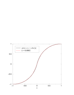
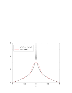
Figure 1: We compare the singular solution of our simple toy problem to the complete solution (for $\epsilon=2\times 10^{-4}$) of the higher order (non-singular) equation. While the two functions agree well over the entire range (left panel), the derivatives obviously differ near the singular point at the origin (right panel). The figures illustrate that the singular solution provides an acceptable approximation to the true solution well away from a region near the origin.

IV The r-modes of nonbarotropic relativistic stars

The discussion in the previous two sections has crucial implications for our attempt to solve the relativistic r-mode problem for nonbarotropic stars. Clearly, we can use our two solutions to Eq. (5) to approximate the physical solution to the problem away from $r=r_{0}$ even though one of these expansions is technically singular at $r_{0}$. This provides us with the means to continue the numerical solution of Eq. (5) across $r=r_{0}$, even though we will not be able to infer the exact form of the solution in a thin thinlayer “boundary layer” near this point. Should we require this information we must carry the slow-rotation calculation to higher orders and solve a much more complicated problem.

We thus propose the following strategy for solving the relativistic r-mode problem in nonbarotropic stars: First integrate the regular solution from the origin up to $r=r_{0}-\delta$, where $\delta$ is suitably small. Then use the numerical solution to fix the two constants $a_{0}$ and $b_{0}$ in the linear combination (cf. (11) and (21) )

$$h=h^{\rm reg}+h^{\rm sing}$$ (42)

Finally, this approximate solution is used to re-initiate numerical integration at $r_{0}+\delta$. This approach was first advocated by one of us in a set of circulated but unpublished notes nils98 , and the idea was resurrected by Ruoff and Kokkotas kr .

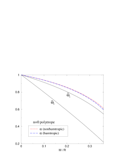
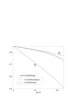
Figure 2: The r-mode eigenfrequencies $\alpha$ of relativistic nonbarotropic stars for $n=0$ (left panel) and $n=1$ polytropes (right panel). Also shown are the corresponding values of the relativistic framedragging at the centre $\tilde{\omega}_{c}$ and surface $\tilde{\omega}_{s}$ of the star. Whenever $\tilde{\omega}_{c}<\alpha<\tilde{\omega}_{s}$ the problem is formally singular. As is clear from the data, the uniform density case ($n=0$) is always regular while most of our $n=1$ models are in the singular range. Also shown (as a dashed curve) are the eigenfrequencies for the axial-led inertial mode of a barotropic star that most resembles the leading Newtonian r-mode. Note that the inertial mode problem is never singular.

We have used the proposed strategy to calculate r-modes for a wide range of polytropic stellar models. Typical results are shown in Figure 2. (Shown also for comparison are the inertial mode frequencies of fully relativistic barotropes lfa . The inertial modes shown are those that limit to the $l=m=2$ r-mode of the corresponding Newtonian barotropic model.) By comparing the obtained mode-eigenvalues $\alpha$ to the values for the relativistic framedragging at the centre and surface of the star ($\tilde{\omega}_{c}$ and $\tilde{\omega}_{s}$, respectively), one can see that the r-mode problem is always regular for uniform density stars. As the equation of state becomes softer ($n$ increases) the situation changes. For example, for $n=1$ polytropes one must typically consider the singular problem in order to find the relativistic r-mode. This conclusion is in agreement with Kokkotas and Ruoff kr as well as Yoshida yosh . It is worth emphasizing that the inertial mode problem for barotropic stars is never singular laf1 ; lfa unless one makes the Cowling approximation khp ; rsk , an approximation that is not in fact appropriate in the barotropic case.

Before discussing our results further we need to comment on a difference between our calculation and those in kr ; yosh . In these papers the authors consider polytropic equations of state of the form

$$p=K\epsilon^{1+1/n}$$ (43)

with $p$ the pressure and $\epsilon$ the energy density. Meanwhile, we are using

$$p=K\rho_{0}^{1+1/n}\quad,\mbox{ and }\quad\epsilon=\rho_{0}+np$$ (44)

where $\rho_{0}$ is the rest-mass density, in order to stay in line with the analysis of the inertial modes of barotropic stars lfa . This means that our numerical results cannot be directly compared to those in kr . In order to verify that the results are consistent we have done some calculations using also (43). We then find that our results are in perfect agreement with those of Ruoff and Kokkotas.

Our calculations thus support the numerical results of the previous studies. It is clear that, for more realistic equations of state one must consider the singular r-mode problem. Where we differ from both Ruoff and Kokkotas kr and Yoshida yosh is in the interpretation of the results in these cases. Yoshida only considers the regular problem, and tentatively argues that there may not exist any relativistic r-modes when the problem is singular. Similar conclusions are drawn by Ruoff and Kokkotas kr . As we have already indicated, we disagree with these conclusions. Even in the slow rotation approximation the perturbations, obtained by solving the initial value problem, are non-singular. However, the root cause of the singular nature of the mode problem is a breakdown in the slow-rotation approximation. We believe that this problem would not arise if the calculation were taken to higher orders in $\Omega$ in the vicinity of the “singular” point (in analogy with boundary layer studies in problems involving viscous fluid flows). The physical problem is likely to be perfectly regular, but unless we extend the slow-rotation calculation to higher orders (or approach the problem in a way that avoids the slow-rotation expansion) we cannot solve the r-mode problem completely for nonbarotropic stars. However, we have shown how the r-mode eigenfrequencies can be estimated using only the solution to the singular mode problem, where they manifest themselves as zero-step solutions.

The case in favor of our approach has been argued (we believe convincingly) in the previous sections. In addition, we can provide one further piece of evidence. In our previous study laf1 , it was pointed out that there is a striking similarity between the eigenfunctions of modes in barotropic and nonbarotropic stars. For example, the metric variable $h(r)$ for an $l=m=2$ r-mode of a nonbarotropic uniform density star was very similar to that of the axial-led hybrid mode corresponding to the Newtonian $l=m=2$ r-mode. This is exactly what one would expect if the two represent a related physical mode-solution. We can now extend this comparison to the case of polytropic stars. The relevant data are shown in Figure 3. We believe these data provide further support for the relevance of our nonbarotropic relativistic r-mode results.

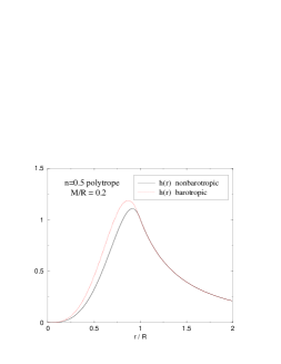
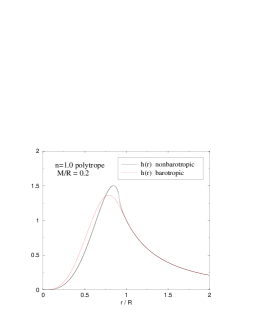
Figure 3: The eigenfunction for an r-mode of a relativistic nonbarotropic star is compared to the corresponding axial-led hybrid mode of a barotropic model. In each comparison, the equilibrium model is chosen to be the same: a relativistic polytrope of compactness $M/R=0.2$ and polytropic index $n=0.5$ (left panel) or $n=1.0$ (right panel). The left panel shows a case in which the nonbarotropic mode is regular while the right panel shows a case in which the nonbarotropic mode is singular (the singular point is close to the surface at $r_{0}=0.913R$.) The functions are all normalized so that $h(R)=1$.

V Conclusions and caveats

We have discussed the calculation of r-modes of relativistic nonbarotropic stars, shedding new light on a problem that has been associated with some confusion in the literature. We have shown how the seemingly singular problem can (in principle) be regularized, using standard ideas from boundary layer theory and viscous fluid flows, and how one can nonetheless estimate the eigenfrequencies of the desired r-modes from the singular mode problem. There are however issues that remain to be resolved, two of which merit particular comment.

Kojima’s equation admits a continuous spectrum of singular solutions whose collective perturbation is non-singular. The time-dependence of the collective perturbation is complicated, but includes a position dependent frequency contribution, and possible power law decay with time. At certain frequencies within the continuous spectrum one can find perturbations that behave like stable modes, whose manifestation is again non-singular (the zero-step solutions). We have argued in this paper that the underlying physical problem can be regularized by considering higher order rotational corrections. The effect of such regularization on the continuous spectrum and zero-step solutions is as yet unclear. If the zero-step solutions become regular normal modes then this would be physically interesting. The fate of the rest of the continuous spectrum is unknown; it may remain, vanish, or break up into discrete normal modes.

The second issue is of relevance should we want to assess the astrophysical importance of the r-modes we have computed. In order to do this we need to estimate the timescale on which the mode grows due to gravitational wave emission lfa ; rk2 . This calculation requires knowledge of the perturbed fluid velocity in order for the relevant canonical mode-energy to be evaluated. In the notation of laf1 , we need the variable $U(r)$. We know from Eq. (4.21) in laf1 that

$$(\alpha-\tilde{\omega})\ U=-\alpha h$$

Clearly if we were to use our mode solution to Eq. (5), the corresponding result for $U$ would necessarily be singular, blowing up like $1/(\alpha-\tilde{\omega})$ at the singular point. In accordance with the arguments in Sections II and III above, it is easy to argue that the “physical” solution $U(r)$ will be smoothed out by including higher order terms near the singular point and thus be regular at all points inside the star. However, solving this higher order problem is difficult. We can in principle avoid having to solve the higher order problem by solving instead the time-dependent initial value problem for the physical velocity perturbation. The physical velocity perturbation, just like the metric perturbation, will be non-singular. Unfortunately solution of the initial value problem is very difficult if one does not have a full analytic solution for the singular mode problem (see w2 where the same issues are discussed for the differential rotation problem). This may well mean that we cannot meaningfully estimate the gravitational radiation reaction timescale for the singular nonbarotropic modes discussed in this paper.

*

Appendix A Continuous spectra in the barotropic problem

Although in this paper we focus on the nonbarotropic problem, a brief note on the barotropic problem is in order. The barotropic normal mode problem is not singular at lowest order in the slow rotation expansion if one includes the metric perturbations laf1 ; lfa . It is however singular if one makes the Cowling approximation khp ; rsk . The Cowling approximation problem can be regularized by considering the initial value problem khp or by coupling to higher order multipoles rsk . However, Lockitch, Andersson and Friedman laf1 have shown that the Cowling approximation is not appropriate to describe the inertial modes of a barotropic star. The singular problem that arises in this case is thus an artifact associated with an unphysical assumption.

In Ref. rsk , Ruoff, Stavridis and Kokkotas study barotropic inertial modes in the Cowling approximation. They expand the eigenfunctions in terms of spherical harmonics, which leads to a set of coupled equations that they truncate at some value $l_{max}$ of the angular parameter $l$. For a given $l_{max}$, they find certain frequency bands for which the matrix problem cannot be inverted, and claim (correctly) that these frequency bands represent continuous spectra. When $l_{max}$ is increased, these continuous spectra are replaced by a discrete eigenfrequency solution at a frequency close to that previously occupied by the continuous spectrum. However, other continuous spectra now appear at different frequency bands. As $l_{max}$ increases these continuous spectrum bands grow in number and begin to span the full range of frequency space.

The authors do not explain why this should be the case, but note that the continuous spectra may vanish when further higher order couplings are taken into account. In fact they should also vanish in the limit $l_{max}\rightarrow\infty$ with only the lower order couplings that they consider. The continuous spectra that they observe for a given $l_{max}$ are the continuous spectra associated with the inertial modes of highest $l$. By including one more term in the coupling equations these solutions are regularized by coupling to higher order multipoles, hence the appearance of discrete mode frequencies. At the same time a new set of continuous spectra appear, associated with the unregularized inertial modes that have $l=l_{max}$. As $l$ increases there are more and more inertial modes lf , hence the apparent proliferation of continuous spectra. In the limit $l_{max}\rightarrow\infty$ the inertial mode problem will be regular,and concerns that the frequency band may fill up with continuous spectra are unfounded even in the low coupling approximation. In this limit mode ”disappearance” within continuous spectra is no longer an issue. In the limit of finite $l_{max}$ modes may however appear as zero-step solutions within the continuous spectra: this is a topic for further study.