Graceful exit from inflation using quantum cosmology
Abstract
A massless scalar field without self interaction and string coupled to gravity is quantized in the framework of quantum cosmology using the Bohm-de Broglie interpretation. Gaussian superpositions of the quantum solutions of the corresponding Wheeler-DeWitt equation in minisuperspace are constructed. The Bohmian trajectories obtained exhibit a graceful exit from the inflationary Pre-Big Bang epoch to the decelerated expansion phase.
PACS numbers: 98.80.Hw, 04.20.Cv, 04.60.Kz
I Introduction
Superstring theory provides an exciting superinflationary model [1] based on a dilaton field interaction with gravity which is free from the common fine tuning of inflationary models because the potential term does not play a crucial role. The superinflationary cosmological solutions come in duality related pairs, or branches; the first one describes a superinflationary expansion and the second branch has a decelerated expansion. The two phases are separated by a singularity.
The graceful exit problem of superinflation [2] consists in obtaining a smooth transition from the two duality solutions. It is usually assumed that this transition can only be possible if strong curvature effects are present (see Ref. [3] for discussion on this point, and other possibilities).
The application of the quantum cosmology approach [4] to the graceful exit problem seems to be a natural choice as long as the strong curvature regime often provides conditions for quantum cosmological effects [5, 6, 7]. One of the main features of quantum cosmology is the possible avoidance of classical singularities due to quantum effects. In order to extract predictions from the wave function of the Universe, the Bohm-de Broglie ontological interpretation of quantum mechanics [8, 9] has been proposed [10, 11], since it avoids many conceptual difficulties that follow from the application of the standard Copenhagen interpretation to a unique system that contains everything. In opposition to the latter one, the ontological interpretation does not need a classical domain outside the quantized system to generate the physical facts out of potentialities (the facts are there ab initio), and hence it can be applied to the Universe as a whole***Other alternative interpretations can be used in quantum cosmology like the Many Worlds interpretation of quantum mechanics [12]. This interpretation admits the concept of trajectories, called Bohmian trajectories, which in the case of cosmology are entire histories of the Universe. These histories satisfy a modified Hamilton-Jacobi equation, different from the classical one due to the presence of a quantum potential term. Hence, the Bohmian trajectories become different from the classical ones when quantum effects become important. Recent investigations [13, 14] have used this approach to investigate issues of string cosmology, among them, the superinflationary behaviour and the possibility of solving the graceful exit problem.
In the present paper we will be restricted to the simple case of no dilaton field potential term and Friedmann-Lemaître-Robertson-Walker (FLRW) geometries with flat spatial sections. The Bohmian trajectories obtained from solutions of the Wheeler-DeWitt (WDW) equation in Jordan’s frame can be calculated through suitable conformal transformations [15] from the Bohmian trajectories in Einstein’s frame, which were obtained in Ref. [16] from Gaussian superpositions of negative and positive mode solutions of the related WDW equation. The resulting trajectories present a smooth transition from the classical inflationary Pre-Big Bang epoch to the usual classical Pos-Big-Bang decelerated phase. A graceful exit is created through quantum effects which are relevant only at the transition.
In Section II we show the duality classical solutions for superinflation in Jordan’s frame. Section III uses the Bohmian trajectories obtained in Ref. [16] in Einstein’s frame to obtain the related trajectories in Jordan’s frame. The graceful exit transition from the superinflation Pre-Big Bang epoch to the usual decelerated expansion phase is exhibited. The conclusions are presented in Section IV.
II The classical model
The so called superinflation is a superstring cosmology duality-pair solution in the low energy effective field theory context. The relevant terms can be shown in the following Lagrangian in the Jordan frame (with non-minimal coupling between gravity and the free scalar field):
| (1) |
This Lagrangian appears in effective string theory without the Kalb-Ramond field when , the usual dilaton field potential not being considered in this paper. Through a conformal transformation , we can obtain the Lagrangian in the Einstein frame (with minimal coupling)
| (2) |
where . To compare with the classical trajectories obtained in Ref. [2], just the case will be studied here, so .
The Robertson-Walker metric with vanishing spatial curvature
| (3) |
will be used in the Jordan frame. The consequence of applying the conformal transformation on the metric (3) must be taken into account when we compare the results in the Jordan and Einstein frames (see Ref. [15]). Then, the lapse function and the scale factor are modified,
| (4) |
yielding and .
Working in the gauge and restricting the scalar field to be time dependent, , the solutions of the equations of motion of the Lagrangian (1) in the Jordan frame are given in Ref. [2], and can be organized in two branches of solutions for as functions of time.
The branch, valid when , reads
| (5) | |||||
| (6) |
and describes accelerated expansion in the case , i.e., inflationary evolution.
For , the branch solution seems to be almost the same,
| (7) | |||||
| (8) |
but now describes decelerated expansion in the case , which can be connected smoothly to a Friedmann-Robertson-Walker (FRW) decelerated expansion.
The transition from an inflationary expanding universe to a FRW expanding one, or graceful exit from inflation, will be obtained here by means of quantum Bohmian trajectories. These trajectories are better described using the coordinate , so that the branch (5)–(6) in the case, gives
| (9) | |||||
| (10) |
while the branch (7)–(8), also in the case, yields
| (11) | |||||
| (12) |
Hence, the classical trajectories in the plane are straight lines with different slopes depending on the type of branch, and both have singularities for .
III Quantum cosmology with the Bohm–de Broglie interpretation
In Ref. [16], the Dirac quantization approach was applied to the theory in the Einstein frame (2), giving the Wheeler-DeWitt equation in minisuperspace whose quantum solutions were obtained. Gaussian superpositions of these solutions given by
| (13) |
with
| (14) |
and arbitrary constants, were interpreted using the Bohm-de Broglie ontological interpretation of quantum mechanics [8, 9], and the resulting system of planar equations for the case of vanishing spatial curvature was :
| (15) | |||||
| (16) |
where , and we have relabeled .
The solutions of the above equations yield the Bohmian trajectories. Among others, there are bouncing regular solutions which contract classically from infinity until a minimum size, where quantum effects become important acting as repulsive forces avoiding the singularity, expanding afterwards to an infinite size, approaching the classical expansion as long as the scale factor increases. For details, see Ref. [16]†††Note that the variables are the variables of Ref. [16], renamed to avoid misunderstanding.. With the lapse function we can obtain the dependence on for and .
To obtain the Bohmian trajectories in Jordan’s frame we only have to make the following substitutions in Eqs. (15)–(16): and (see Eq. (4)). Finally, as we use , we have . The planar system in the variables then reads
| (17) | |||||
| (18) |
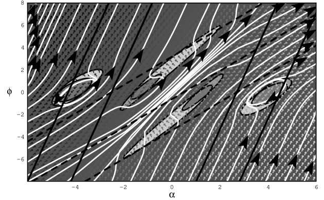
A field plot of this planar system is shown in Figure 1, for . Depending on the initial conditions, there are three types of behaviour for the Bohmian trajectories. There are small oscillating universes without singularities near the center points placed in the axis. When , Eqs. (17)–(18) approach the classical equations of motion yielding the straight lines which appear in Figure 1, representing the classical solutions (10)–(12). Note, however, that in the region of small values of there are smooth transitions between these two straight lines which are not present in the classical solutions. One possible type of transition is exactly the graceful exit, from the branch with inflationary expansion to the branch solution with decelerated expansion. Another possible type of transition is the opposite of the graceful exit, from the branch with decelerated expansion to the branch solution with inflationary expansion.
We can choose one Bohmian trajectory to see the evolution with respect to time . Figures 2 and 3 clearly show the graceful exit behaviour, i.e., the evolution that begins with inflation and smoothly changes to the decelerated expansion without any singularity in the transition. The scale factor and the Hubble parameter of the classical solutions are recovered when , but near there is no singularity.
IV Conclusion
We have shown that the Bohm-de Broglie ontological interpretation of quantum cosmology applied to string cosmology can yield a simple answer to the graceful exit problem in superinflation.
Using a previous study [16] in the Einstein frame, where Gaussian superpositions of the solutions of the Wheeler-DeWitt equation in the minisuperspace allows the determination of Bohmian trajectories, we applied a conformal transformation to obtain in a straightforward way the Bohmian trajectories in the Jordan frame corresponding to universe histories in string cosmology.
We exhibited a class of trajectories representing universe evolutions with graceful exit. They start classically from inflationary behaviour driven by kinetic terms, as it is usual in these cases. When curvature becomes relevant, quantum effects become important avoiding the singularity and creating a smooth transition to the usual classical decelerated expansion.
The results of this paper should be contrasted with results obtained using other interpretations (see, e.g., Ref. [7]). In the case of the Many Worlds interpretation, the construction of a Hilbert space is very important in order to define a probability measure. However, for scalar field minisuperspaces, the Wheeler-DeWitt equation has a Klein-Gordon structure and it is well known that it is hard to construct a unique positive definite measure with such equations. The common way out from these problems is to take semiclassical approximations. This problem is intimately connected with the problem of time [17]. Once we do not have an extrinsic time, the Wheeler-DeWitt equation cannot be transformed into a Schroedinger like equation, and hence all these problems with its hyperbolic signature appear, unless one makes use of a semiclassical approximation as it is done in Ref. [7]. However, the graceful exit shall occur when quantum effects are important, where a semiclassical approximation breaks down, rendering problematic the analysis of this transition in the Many Worlds interpretation. In the Bohm-de Broglie interpretation, probability measures are not essential. We can talk about quantum trajectories, and probabilities are relevant only for settling reasonable initial conditions on such trajectories. The notion of quantum trajectories is well defined even for Klein-Gordon like Wheeler-DeWitt equations. The scale factor and scalar field follow real trajectories which satisfy modified Einstein’s equations ammended with a quantum potential term. The concept of spacetime is as meaningfull in the Bohm-de Broglie interpretation of minisuperspace quantum cosmology as it is in classical General Relativity (GR) (see Ref. [18] for a detailed discussion on this point, and [10] for the different case of midisuperspace models and the full superspace). The only difference is that the dynamics may be changed by the presence of the quantum potential. As in classical minisuperspace GR, the dynamics is invariant under time reparametrizations, even in the presence of the quantum potential. Hence, the symbol in the Bohmian trajectories is an arbitrary parameter like in GR, which can be fixed by a choice of the lapse function, without physical modifications of the dynamics of spacetime. That is how it is possible, in this interpretation, to talk about a graceful exit transition when the curvature of spacetime increases. We have only to examine the behaviour of the Bohmian trajectories in such regions. Note that in the region of configuration space where a semiclassical description can be applied in the framework of the Many Worlds interpretation, there is accordance of results: the semiclassical wave function is peaked along the classical trajectories [7], which are exactly the Bohmian trajectories in that region.
The conclusion is that, as the Bohm-de Broglie interpretation has more concepts then the Many Worlds interpretation, the former can be used in situations where the application of the latter is problematic. Our results come in this way. Of course it would be desirable to define a probability measure on the Bohmian trajectories coming from the wave function (13), which could be valid in all minisuperspace, as long as not all of them describe the Pre-Big Bang model with graceful exit, although all Bohmian trajectories with initial conditions imposing an initial superinflationary Pre-Big Bang phase present a graceful exit to the decelerated regime. If this is possible, one should expect that the statistical predictions of the Many Worlds interpretation are identical to the statistical predictions of the Bohm-de Broglie interpretation.
The above considerations raise doubts on the physical equivalence of these two interpretations in quantum cosmology. Due to the singular features present in the quantization of the whole Universe, it is possible that one of them presents more physical relevant and testable information then the other in this particular field (which is not the case, up to now, in quantum field theory and non relativistic quantum mechanics). This suggests that quantum cosmology may be the arena where it could be possible to distinguish physically between these two interpretations. This is a strong motivation to push forward these two interpretations up to their limits in all possible aspects of quantum cosmology and compare their results in order to obtain a relevant physical distinction, or even some observable prediction, which could select one of them as the valid interpretation of quantum mechanics.
A logical future generalization of the present work is to study dilaton field potential terms so that the decelerated expansion can be joined smoothly to an ordinary FRW radiation dominated expanding Universe [2]. It is also important to check how these results depend on initial conditions on the WDW equation.
ACKNOWLEDGMENTS
We would like to thank CNPq and CAPES of Brazil for financial support. One of us (NPN) would like to thank the Laboratoire de Gravitation et Cosmologie Relativistes of Université Pierre et Marie Curie where part of this work has been done, for financial aid and hospitality, and the group of “Pequeno Seminário” in CBPF for useful discussions.
REFERENCES
- [1] G. Veneziano, Phys. Lett. B265, 287 (1991).
- [2] R. Brustein and G. Veneziano, Phys. Lett. B329, 429 (1994).
- [3] I. Antoniadis, J. Rizs and K. Tomvakis, Nucl. Phys. B415, 497, (1994); E. Kritsis and C. Kounnas, Phys. Lett B331, 51 (1994); G. F. R. Ellis, D. C. Roberts, D. Solomons and P. K. S. Dunsby, preprint gr-qc/9912005.
- [4] J. A. Wheeler, in Battelle Rencontres: 1967 Lectures in Mathematical Physics, ed. by B. DeWitt and J. A. Wheeler (Benjamin New York, 1968); B. S. DeWitt, Phys. Rev. 160, 1113 (1967).
- [5] M. Gasperini and G. Veneziano, Gen. Rel. Grav. 28, 1301 (1996).
- [6] J. E. Lidsey, Phys. Rev. D55, 3303 (1997).
- [7] M. P. Da̧browski and C. Kiefer, Phys. Lett. B397, 185 (1997).
- [8] D. Bohm, Phys. Rev. 85, 166 (1952); D. Bohm, B. J. Hiley and P. N. Kaloyerou, Phys. Rep. 144, 349 (1987).
- [9] P. R. Holland, The Quantum Theory of Motion: An Account of the de Broglie-Bohm Causal Interpretation of Quantum Mechanics (Cambridge University Press, Cambridge, 1993).
- [10] N. Pinto-Neto and E. S. Santini, Phys. Rev. D59, 123517 (1999).
- [11] J. A. de Barros, N. Pinto-Neto and M. A. Sagioro-Leal, Phys. Lett. A241, 229 (1998).
- [12] The Many-Worlds Interpretation of Quantum Mechanics, ed. by B. S. DeWitt and N. Graham (Princeton University Press, Princeton, 1973).
- [13] J. Marto and P. Moniz, Opening the graceful exit with Broglie-Bohm quantum string cosmology, to appear in the Proceedings of the Marcel Grossmann MG9 Conference, Rome, 2000.
- [14] J. Marto and P. Moniz, Broglie-Bohm FRW Universe in Quantum String Cosmology, preprint GATC-DF-UBI-02/2001, submitted to publication.
- [15] J. C. Fabris, N. Pinto-Neto and A. F. Velasco, Class. and Quantum Grav., 16, 3807, (1999).
- [16] R. Colistete Jr., J. C. Fabris and N. Pinto-Neto, Phys. Rev. D62, 83507 (2000).
- [17] K. Kuchar in Quantum Gravity 2: a Second Oxford Symposium, C. J. Isham, R. Penrose and D. W. Sciama (Clarendon Press, Oxford, 1981).
- [18] J. A. de Barros and N. Pinto-Neto, Int. J. Mod. Phys. D7, 201 (1998).