Boundary conditions in linearized harmonic gravity

Abstract

We investigate the initial-boundary value problem for linearized gravitational theory in harmonic coordinates. Rigorous techniques for hyperbolic systems are applied to establish well-posedness for various reductions of the system into a set of six wave equations. The results are used to formulate computational algorithms for Cauchy evolution in a 3-dimensional bounded domain. Numerical codes based upon these algorithms are shown to satisfy tests of robust stability for random constraint violating initial data and random boundary data; and shown to give excellent performance for the evolution of typical physical data. The results are obtained for plane boundaries as well as piecewise cubic spherical boundaries cut out of a Cartesian grid.

I Introduction

Grid boundaries pose major difficulties in current computational efforts to simulate 3-dimensional black holes by conventional Cauchy evolution schemes. The initial-boundary value problem for Einstein’s equations consists of the evolution of initial Cauchy data on a spacelike hypersurface and boundary data on a timelike hypersurface. This problem has only recently received mathematical attention. Friedrich and Nagy [1] have given a full solution for a hyperbolic formulation of the Einstein equations based upon a frame decomposition in which the connection and curvature enter as evolution variables. Because this formulation was chosen to handle mathematical issues rather than for ease of numerical implementation, it is not clear how the results translate into practical input for formulations on which most computational algorithms are based. The proper implementation of boundary conditions depends on the particular reduction of Einstein’s equations into an evolution system and the choice of gauge conditions. The purpose of this paper is to elucidate, in a simple context, such elementary issues as: (i) which variables can be freely specified on the boundary; (ii) how should the remaining variables be updated in a computational scheme; (iii) how can the analytic results be implemented as a computational algorithm. For this purpose, we consider the evolution of the linearized Einstein’s equations in harmonic coordinates [2, 3] and demonstrate how a robustly stable and highly accurate computational evolution can be based upon a proper mathematical formulation of the initial-boundary value problem.

Harmonic coordinates were used to obtain the first hyperbolic formulation of Einstein’s equations [4]. See Ref. [5] for a full account of hyperbolic formulations of general relativity. While harmonic coordinates have also been widely applied in carrying out analytic perturbation expansions, they have had little application in numerical relativity, presumably because of the restriction in gauge freedom [6]. However, there has been no ultimate verdict on the suitability of harmonic coordinates for computation. In particular, their generalization to include gauge source functions [7] appears to offer flexibility comparable to the explicit choice of lapse and shift in conventional numerical approaches to general relativity. There is no question that harmonic coordinates offer greater computational efficiency than any other hyperbolic formulation. See Ref. [8] for a recent application to the study of singularities in a space-time without boundary. Here we use a reduced version of the harmonic formulation of the field equations. This allows us retain a symmetric hyperbolic system, and apply standard boundary algorithms, in a way that is consistent with the propagation of the constraints. We show, on an analytic level, that this leads to a well posed initial-boundary problem for linearized gravitational theory.

Our computational results are formulated in terms of a Cartesian grid based upon background Minkowskian coordinates. Robustly stable evolution algorithms are obtained for plane boundaries aligned with the Cartesian coordinates, which is the standard setup for three dimensional evolution codes. Similar computational results [9], based upon long evolutions with random initial and boundary data, were previously found for the linearized version of the Arnowitt-Deser-Misner formulation (ADM) [10] of the field equations, where the lack of a hyperbolic formulation required a less systematic approach which had no obvious generalization to other boundary shapes. In this paper, we also attain robust stability for spherical boundaries which are cut out of the Cartesian grid in an irregular piecewise cubic fashion. This success gives optimism that the methods can applied to such problems as black hole excision and Cauchy-characteristic matching, where spherical boundaries enter in a natural way.

Conventions: We use Greek letters for space-time indices and Latin letters for spatial indices, e.g. $x^{\alpha}=(t,x^{i})$ for standard Minkowski coordinates. Linear perturbations of a curved space metric $g_{\alpha\beta}$ about the Minkowski metric $\eta_{\alpha\beta}$ are described by $\delta g_{\alpha\beta}=h_{\alpha\beta}$ with similar notation for the corresponding curvature quantities, e.g. the linearized Riemann tensor $\delta R_{\alpha\beta\gamma\delta}$ and linearized Einstein tensor $\delta G_{\alpha\beta}$. Indices are raised and lowered with the Minkowski metric, with the result that $\delta g^{\alpha\beta}=-h^{\alpha\beta}$. Boundaries in the background geometry are described in the form $z=const$ with the spatial coordinates decomposed in the form $x^{i}=(x^{A},z)$, where the $x^{A}=(x,y)$ directions span the space tangent to the boundary.

II Harmonic evolution without boundaries

The linearized Einstein tensor has the form

$$\delta G^{\alpha\beta}=-\frac{1}{2}\Box\gamma^{\alpha\beta}-\partial^{(\alpha}\Gamma^{\beta)}+\frac{1}{2}\eta^{\alpha\beta}\partial_{\mu}\Gamma^{\mu},$$ (1)

where $\Box=\partial_{\mu}\partial^{\mu}$

$$\gamma^{\alpha\beta}=h^{\alpha\beta}-\frac{1}{2}\eta^{\alpha\beta}h$$ (2)

$h=h^{\alpha}_{\alpha}=-\gamma^{\alpha}_{\alpha}=-\gamma$ and

$$\Gamma^{\alpha}=-\partial_{\beta}\gamma^{\alpha\beta}.$$ (3)

We analyze these equations in standard background Minkowskian coordinates $x^{\alpha}$. To linearized accuracy,

$$\Gamma^{\alpha}\approx g^{\mu\nu}\nabla_{\mu}\nabla_{\nu}x^{\alpha}$$ (4)

in terms of the curved space connection $\nabla_{\mu}$ associated with $g_{\alpha\beta}$ and the condition $\Gamma^{\alpha}=0$ defines a linearized harmonic gauge.

The diffeomorphisms of the curved spacetime induce equivalent metric perturbations according to the harmonic subclass of gauge transformations

$$\hat{h}^{\alpha\beta}=h^{\alpha\beta}+2\partial^{(\alpha}\xi^{\beta)},$$ (5)

where the vector field $\xi^{\alpha}$ satisfies $\Box\xi^{\alpha}=0$. The linearized curvature tensor

$$2\delta R_{\mu\alpha\nu\beta}=\partial_{\mu}\partial_{\beta}h_{\alpha\nu}+\partial_{\alpha}\partial_{\nu}h_{\mu\beta}-\partial_{\alpha}\partial_{\beta}h_{\mu\nu}-\partial_{\mu}\partial_{\nu}h_{\alpha\beta},$$ (6)

as well as the linearized Einstein equations, are gauge invariant.

We introduce a Cauchy foliation $t$ in the perturbed spacetime such that it reduces to an inertial time slicing in the background Minkowski spacetime. The unit normal to the Cauchy hypersurfaces is given, to linearized accuracy, by

$$n_{\alpha}\approx-(1+\frac{1}{2}h^{tt})\partial_{\alpha}t.$$ (7)

The choice of an evolution direction $t^{\mu}=\alpha n^{\mu}+\beta^{\mu}$, with unit lapse and shift in the background Minkowski spacetime, defines a perturbative lapse $\delta\alpha=-h^{tt}/2$ and perturbative shift $\delta\beta^{i}=-h^{ti}$.

A Standard harmonic evolution

Harmonic evolution consists of solving the Einstein’s equations $G_{\alpha\beta}=0$, subject to the harmonic conditions $\Gamma^{\alpha}=0$. This formulation led to the first existence and uniqueness theorems for solutions to the nonlinear Einstein equations by considering them as a set of 10 nonlinear wave equations [11].

In the linearized case, Einstein’s equations in harmonic coordinates reduce to ten flat space wave equations so that their mathematical analysis is simple. The Cauchy data $\gamma^{\alpha\beta}(0,x^{i})$ and $\partial_{t}\gamma^{\alpha\beta}(0,x^{i})$ at $t=0$ determine ten unique solutions $\gamma^{\alpha\beta}(t,x^{i})$ of the wave equation $\Box\gamma^{\alpha\beta}=0$, in the appropriate domain of dependence. These solutions satisfy $\Box\Gamma^{\alpha}=0$ so that they satisfy Einstein’s equations provided $\Gamma^{\alpha}(0,x^{i})=0$ and $\partial_{t}\Gamma^{\alpha}(0,x^{i})=0$, which can be arranged by choosing initial Cauchy data satisfying constraints. For a detailed discussion, see Ref. [12].

Although this standard harmonic evolution scheme led to the first existence and uniqueness theorem for Einstein’s equations, it is not straightforward to apply to the initial-boundary value problem. The ten wave equations for $\gamma^{\alpha\beta}$ require ten individual pieces of boundary data in order to determine a unique solution. Given initial data such that $\Gamma^{\alpha}=0$ and $\partial_{t}\Gamma^{\alpha}=0$ at $t=0$, as described above, the resulting solution satisfies the linearized Einstein equations only in the domain of dependence of the Cauchy data. In order that the solution of Einstein’s equations extend to the boundary, it is necessary that $\Gamma^{\alpha}=0$ at the boundary. Unfortunately, there is no version of boundary data for $\gamma^{\alpha\beta}$, e.g. Dirichlet, Neumann or Sommerfeld data for the ten individual components, from which $\Gamma^{\alpha}$ can be calculated at the boundary. Here we consider reduced versions of the harmonic evolution scheme in which only six wave equations are solved and this problem does not arise. These reduced harmonic formulations are presented below.

B Reduced harmonic Einstein evolution

A linearized evolution scheme for the harmonic Einstein system, can be based upon the six wave equations

$$\Box\gamma^{ij}=0$$ (8)

along with the four harmonic conditions

$$\partial_{\mu}\gamma^{\mu\nu}=0.$$ (9)

Because of the harmonic conditions, this system satisfies the spatial components $\delta G^{ij}=0$ of the linearized Einstein’s equations.

As a result of the linearized Bianchi identities $\partial_{\alpha}\delta G^{\alpha\beta}=0$, or

$$\partial_{t}\delta G^{it}+\partial_{j}\delta G^{ij} = 0$$ (10)

$$\partial_{t}\delta G^{tt}+\partial_{j}\delta G^{tj} = 0,$$ (11)

the linearized Hamiltonian constraint ${\cal C}:=\delta G^{tt}=0$ and linearized momentum constraints ${\cal C}^{i}:=\delta G^{ti}=0$ are also satisfied, throughout the domain of dependence of the Cauchy data, provided that they are satisfied at the initial time $t=0$. This constrains the initial values of $\gamma^{t\alpha}$ according to

$$\nabla^{2}\gamma^{ti}+\partial_{t}\partial_{j}\gamma^{ij}=0$$ (12)

and

$$\nabla^{2}\gamma^{tt}-\partial_{i}\partial_{j}\gamma^{ij}=0,$$ (13)

where $\nabla^{2}=\delta^{ij}\partial_{i}\partial_{j}$. Then, if these constraints are initially satisfied, the reduced harmonic Einstein system determines a solution of the linearized Einstein’s equations.

The well-posedness of the system follows directly from the well-posedness of the wave equations for $\gamma^{ij}$. The auxiliary variables $\gamma^{\alpha t}$ satisfy the ordinary differential equations

$$\partial_{t}\gamma^{it}+\partial_{j}\gamma^{ij} = 0$$ (14)

$$\partial_{t}\gamma^{tt}+\partial_{j}\gamma^{tj} = 0,$$ (15)

where $\gamma^{ij}$ enters only in the role of source terms. These differential equations do not affect the well-posedness of the system and have unique integrals determined by the initial values of $\gamma^{\alpha t}$.

C Reduced harmonic Ricci evolution

The reduced harmonic Ricci system consists of the six wave equations

$$\Box h^{ij}=0$$ (16)

along with the four harmonic conditions (9), which can be re-expressed in the form

$$\partial_{t}\phi+\partial_{j}h^{jt}+\frac{1}{2}\,\partial_{t}h^{j}_{j}=0,$$ (17)

$$\partial^{i}\phi+\partial_{t}h^{it}-\frac{1}{2}\,\partial^{i}h^{j}_{j}+\partial_{j}h^{ij}=0,$$ (18)

where we have set $\phi=h^{tt}/2$. Together these equations imply that the spatial components of the perturbed Ricci tensor vanish, $\delta R^{ij}=0$. In addition, the Bianchi identities imply that the remaining components satisfy

$$\partial_{t}{\cal C}^{i}+\partial^{i}{\cal C}+\partial_{j}\delta R^{ij} = 0$$ (19)

$$\partial_{t}{\cal C}+\partial_{j}{\cal C}^{j} = 0,$$ (20)

where, in terms of the Ricci tensor, ${\cal C}=\frac{1}{2}(\delta R^{tt}+\delta R^{i}_{i})$ and ${\cal C}^{i}=\delta R^{ti}$. Together with the evolution equations $\delta R^{ij}=0$, the Bianchi identities imply that the Hamiltonian constraint satisfies the wave equation $\Box{\cal C}=0$.

If the Hamiltonian and momentum constraints are satisfied at the initial time, then $\partial_{t}{\cal C}$ also vanishes at the initial time so that the uniqueness of the solution of the wave equation ensures the propagation of the Hamiltonian constraint. In turn, Eq. (19) then ensures that the momentum constraint is propagated. Thus the reduced harmonic Ricci system of six wave equations and four harmonic equations leads to a solution of the linearized Einstein’s equations for initial Cauchy data satisfying the constraints.

The harmonic Ricci system takes symmetric hyperbolic form when the wave equations are recast in first differential order form. Thus the system is well posed. The formulation of the harmonic Ricci system as a symmetric hyperbolic system and the description of its characteristics is given in Appendix A. Although well-posedness of the analytic problem does not the guarantee the stability of a numerical implementation it can simplify its attainment.

D Other reduced harmonic systems

The harmonic Einstein and Ricci systems are special cases of a one parameter class of reduced harmonic systems for the variable

$$\kappa^{\alpha\beta}=\gamma^{\alpha\beta}-\frac{\lambda}{2}\eta^{\alpha\beta}\gamma$$

which satisfying the wave equations $E^{ij}=-\frac{1}{2}\Box\kappa^{ij}=0$ and the harmonic conditions $\Gamma^{\alpha}=0$, where $E^{\alpha\beta}=\delta G^{\alpha\beta}-\frac{\lambda}{2}\eta^{\alpha\beta}\delta G$. This system is symmetric hyperbolic when the auxiliary system $\Gamma^{\alpha}=0$ is symmetric hyperbolic. This can be analyzed by setting $\kappa^{ij}=0$ in the auxiliary system, which then takes the form

$$0 = \frac{(2-3\lambda)}{2(1-2\lambda)}\partial_{t}\kappa^{tt}+\partial_{j}\kappa^{tj}$$ (21)

$$0 = \partial_{t}\kappa^{ti}-\frac{\lambda}{2(1-2\lambda)}\partial^{i}\kappa^{tt},$$ (22)

and implies

$$(\partial_{t}^{2}-\frac{\lambda}{(3\lambda-2)}\partial_{i}\partial^{i})\kappa^{tt}=0.$$ (23)

The auxiliary system is symmetric hyperbolic when Eq. (23) is a wave equation whose wave speed

$$v=\sqrt{\frac{\lambda}{(3\lambda-2)}}$$ (24)

is positive. This is satisfied for $\lambda<0$ and $\lambda>2/3$. In the range $2/3<\lambda<1$, the wave speed is faster than the speed of light. Only for the case $\lambda=1$, the harmonic Ricci system, is the wave speed of the auxiliary system equal to the speed of light.

The auxiliary system for the reduced harmonic Einstein case has a well posed initial-boundary value problem but represents a borderline case. This could adversely affect the development of a stable code based upon a nonlinear version of the reduced harmonic Einstein system.

III The initial-boundary value problem

Consider the initial-boundary problem consisting of evolving Cauchy data prescribed in a set ${\cal S}$ at time $t=0$ lying in the half-space $z>0$ with data prescribed on a set ${\cal T}$ on the boundary $z=0$. Harmonic evolution takes its simplest form when Einstein equations are expressed as a second differential order system. However, in order to apply standard methods it is necessary to recast the problem as a first order symmetric hyperbolic system. Then the theory determines conditions on the boundary data for a well posed problem in the future domain of dependence ${\cal D}^{+}$. Here ${\cal D}^{+}$ is the maximal set of points whose past directed inextendible characteristic curves all intersect the union of ${\cal S}$ and ${\cal T}$ before leaving ${\cal D}^{+}$.

Appendix A describes the symmetric hyperbolic description of boundary conditions for the 3-dimensional wave equation. The basic ideas and their application to the initial-boundary value problem are simplest to explain in terms of the 1-dimensional wave equation, as follows. See Appendix A for the analogous treatment of the 3-dimensional case. Our presentation is based upon the formulation of maximally dissipative boundary conditions [13], the approach used by Friedrich and Nagy [1] in the nonlinear case. An alternative description of boundary conditions for symmetric hyperbolic systems is given in Ref. [14] and for linearized gravity in Ref. [15].

A The 1-dimensional wave equation

The one-dimensional wave equation $h_{,tt}=h_{,zz}$ can be recast as the first order system of evolution equations

$$\dot{h} = k$$ (25)

$$\dot{k} = f_{,z}$$ (26)

$$\dot{f} = k_{,z},$$ (27)

where we have introduced the auxiliary variables $k$ and $f$. Given initial data $(h,k,f)$ at time $t=0$ subject to the constraint, $f=h_{,z}$, these equations determine a solution $h$ of the wave equation. Note that the constraint is propagated by the evolution equations.

In coordinates $x^{\mu}=(x^{0},x^{1})=(t,z)$ the system (25)-(27) has the symmetric hyperbolic form

$$A^{\mu}\partial_{\mu}u=Bu+F,$$ (28)

where the solution $u$ consists of the column matrix

$$u=\left(\;\begin{array}[]{l}h\\ k\\ f\end{array}\right)$$ (29)

and

$$A^{0}=\left(\;\begin{array}[]{ccc}1&0&0\\ 0&1&0\\ 0&0&1\end{array}\right),\quad A^{1}=\left(\;\begin{array}[]{ccc}0&0&0\\ 0&0&-1\\ 0&-1&0\end{array}\right),\quad B=\left(\;\begin{array}[]{ccc}0&1&0\\ 0&0&0\\ 0&0&0\end{array}\right).$$ (30)

In our case the source term $F=0$ but otherwise it plays no essential role in the analysis of the system.

The contraction of Eq. (28) with the transpose ${}^{T}u$ give the flux equation

$${}^{T}uA^{\mu}\partial_{\mu}u={}^{T}u({}^{T}B+B)u.$$ (31)

This can be used to provide an estimate on the norm $\int{}^{T}uA^{0}udz$ for establishing a well posed problem, in the half-space $z>0$ with boundary at $z=0$, provided the flux arising with the normal component of $A^{\mu}$ satisfies the inequality

$${}^{T}uA^{1}u\leq 0.$$ (32)

This inequality determines the allowed boundary data for a well posed initial-boundary value problem.

As expected from knowledge of the characteristics of the wave equation, the normal matrix $A^{1}$ has eigenvalues $0,\pm 1$, with the corresponding eigenvectors

$$v_{0}=\left(\begin{array}[]{r}1\\ 0\\ 0\end{array}\right),\quad v_{\pm 1}=\left(\begin{array}[]{r}0\\ \mp 1\\ 1\end{array}\right).$$ (39)

These eigenvectors are associated with the variables

$$h_{0}=h,\quad h_{\pm 1}=f\mp k=h_{,z}\mp h_{,t}.$$ (40)

Re-expressing the solution vector in terms of the eigenvectors,

$$\tilde{u}=\left(\begin{array}[]{l}h_{-1}\\ h_{0}\\ h_{+1}\end{array}\right)=\left(\begin{array}[]{c}h_{,z}+h_{,t}\\ h\\ h_{,z}-h_{,t}\end{array}\right)$$ (41)

the inequality (32 implies that homogeneous boundary data must take the form

$$0=h_{+1}-Hh_{-1},$$ (42)

where the parameter $H$ satisfies $H^{2}\leq 1$. The component $h_{0}$, corresponding to the kernel of $A^{1}$, propagates directly up the boundary and cannot be prescribed as boundary data.

Non-homogeneous boundary data can be given in the form

$$q(t)=h_{+1}-Hh_{-1}=h_{,z}(1-H)-h_{,t}(1+H),$$ (43)

where $q$ is an arbitrary function representing the free boundary data at $z=0$. Eq. (43) shows how the scalar wave equation accepts a continuous range of boundary conditions. The well-known cases of Sommerfeld, Dirichlet or Neumann boundary data are recovered by setting $H=0,+1$, or, $-1$, respectively. Note that there are consistency conditions at the edge $(t=0,z=0)$. For instance, Dirichlet data corresponds to specifying $k=h_{,t}$ on the boundary and this must be consistent with the initial data for $k$.

B The reduced harmonic Einstein system

The harmonic Einstein system consists of the six wave equations (8) and the four harmonic conditions (9). Since the wave equations for $\gamma^{ij}$ are independent of the auxiliary variables $\gamma^{t\alpha}$, the well-posedness of the initial-boundary value problem for $\gamma^{ij}$ follows immediately. Furthermore, since the harmonic conditions propagate the auxiliary variables up the boundary by ordinary differential equations, the harmonic Einstein system has a well posed initial-boundary value problem. A unique solution in the appropriate domain of dependence is determined by the initial Cauchy data $\gamma^{ij}$ and $\gamma^{ij}_{,t}$ at $t=0$, the initial data $\gamma^{t\alpha}$ at the edge $t=z=0$ and the boundary data $\gamma^{ij}$ at $z=0$ given in any of the forms described in Appendix A (e.g. Dirichlet, Neumann, Sommerfeld).

A solution of the linearized harmonic Einstein system satisfies $\delta G^{ij}$ =0. As a result the Bianchi identities imply $\partial_{t}C^{i}=0$ and $\partial_{t}C=-\partial_{j}C^{j}$ so that the constraints are satisfied provided the constraint Eq’s. (12) and (13) are satisfied at $t=0$.

The free boundary data for this system consists of six functions. However, as shown in Ref. [1], the vacuum Bianchi identities satisfied by the Weyl tensor imply that only two independent pieces of Weyl data can be freely specified at the boundary. We give the corresponding analysis for the linearized Einstein system in Appendix B. This makes it clear that only two of the six pieces of metric boundary data are gauge invariant. This is in accord with the four degrees of gauge freedom consisting of the choice of linearized lapse $\delta\alpha=-h^{tt}/2$ (one free function) and linearized shift $\delta\beta^{i}=-h^{ti}$ (three free functions).

A linearized evolution requires a unique lapse and shift, whose values can be specified explicitly as space-time functions or specified implicitly in terms of initial and boundary data subject to dynamical equations. In the case of a harmonic gauge, in order to assess whether explicit space-time specification of the lapse and shift is advantageous for the purpose of numerical evolution, it is instructive to see how it affects the initial-boundary value problem for the reduced harmonic Einstein system. In the linearized harmonic formulation without boundary, a gauge transformation (5) to a shift-free gauge $\gamma^{ti}=0$ is always possible within the domain of dependence of the initial Cauchy data [12]. In the presence of a boundary, consider a gauge transformation with $\xi^{\alpha}=(0,\xi^{i})$, so that

$$\hat{\gamma}^{ti}=\gamma^{ti}+\partial^{t}\xi^{i}.$$ (44)

For harmonic evolution of constrained initial data, both $\xi^{i}$ and $\gamma^{ti}$ satisfy the wave equation. At $t=0$, choose Cauchy data for $\xi^{i}$ satisfying

$$0=\gamma^{ti}+\partial^{t}\xi^{i}$$ (45)

and

$$0=\partial_{t}\gamma^{ti}+\partial_{t}\partial^{t}\xi^{i}=-\partial_{j}\gamma^{ji}-\nabla^{2}\xi^{i}.$$ (46)

On the boundary $z=0$, require that $\xi^{i}$ satisfy

$$0=\gamma^{ti}+\partial^{t}\xi^{i}.$$ (47)

Then $\hat{\gamma}^{ti}=\gamma^{ti}+\partial^{t}\xi^{i}$ has vanishing Cauchy data at $t=0$, vanishing Dirichlet boundary data at $z=0$ and satisfies the wave equation, so that $\hat{\gamma}^{ti}=0$. Thus, for evolution of constrained data with a boundary, a shift-free harmonic gauge is possible.

However, in this gauge, boundary data for all 6 components of $\gamma^{ij}$ can no longer be freely specified since the harmonic condition implies

$$\partial_{z}\gamma^{zj}+\partial_{A}\gamma^{Aj}=0.$$ (48)

This relates Neumann data for $\gamma^{zj}$ to Dirichlet data for $\gamma^{AB}$ and would complicate any shift-free numerical evolution scheme. As an example, one could freely specify Dirichlet boundary data for the 3 components $\gamma^{AB}$ and (i) obtain Neumann boundary data $\partial_{z}\gamma^{zA}$ from the $A$-components of Eq. (48), (ii) evolve $\gamma^{zA}$ in terms of initial Cauchy data and (iii) obtain Neumann boundary data $\partial_{z}\gamma^{zz}$ from the $z$-component of Eq. (48). Note the nonlocality of step (ii), which would have to be carried out “on the fly” during a numerical evolution.

The requirement that the shift vanish reduces the free boundary data to three components. It is also possible to eliminate an additional free piece of data by choosing a unit lapse, i.e. setting $h^{tt}=0$. Suppose the shift has been set to zero, so that the harmonic condition implies $\partial_{t}h^{tt}=-\partial_{t}h^{i}_{i}$. Consider a gauge transformation $\hat{h}^{tt}=h^{tt}-2\partial_{t}\xi^{t}$, where $\xi^{\alpha}=(\xi^{t},\xi^{i})$ satisfies $\partial_{t}\xi^{i}=\partial^{i}\xi^{t}$ so that the shift remains zero. For harmonic evolution of constrained data, both $\xi^{t}$ and $h^{tt}$ satisfy the wave equation. At $t=0$, choose Cauchy data for $\xi^{t}$ satisfying

$$0=h^{tt}-2\partial_{t}\xi^{t}$$ (49)

and

$$0=\partial_{t}h^{tt}-2\partial^{2}_{t}\xi^{t}=-\partial_{t}h^{i}_{i}-2\nabla^{2}\xi^{t}$$ (50)

(where we assume the Cauchy data is given on a non-compact set so that there are no global obstructions to a solution $\xi^{t}$). On the boundary $z=0$, require $\xi^{t}$ satisfy

$$0=h^{tt}-2\partial_{t}\xi^{t}.$$ (51)

Then $\hat{h}^{tt}=0$ because it is a solution of the wave equation with vanishing Cauchy data and Dirichlet boundary data. (Alternatively, the lapse can be gauged to unity by a transformation satisfying $\Gamma^{t}=\Box\xi^{t}=const$, so that the harmonic source function $\Gamma^{t}$ still drops out of Eq. (1) for the Einstein tensor.)

A unit lapse and zero shift implies that $\partial_{t}\gamma^{i}_{i}=0$ so that $\gamma^{i}_{i}$ cannot be freely specified at the boundary. Coupled with our previous results, imposition of a unit lapse and zero-shift reduces the free boundary data to the two trace-free transverse components $\gamma^{AB}-(1/2)\delta^{AB}\gamma^{C}_{C}$, in accord with the two degrees of gauge-free radiative freedom associated with the Weyl tensor. (In addition, the initial Cauchy data must satisfy Eq. (48), $\partial_{t}\gamma^{i}_{i}=0$ and $\nabla^{2}\gamma^{i}_{i}=0$). A similar result arises in the study of the unit-lapse zero-shift initial-boundary value problem for the linearized ADM equations [9]. However, in the case of harmonic evolution, it is clear that explicit specification of the lapse and shift leads to a more complicated initial-boundary value problem. It is more natural to retain the freedom of specifying 6 pieces of boundary data, which then determine the lapse and shift implicitly during the course of the evolution.

The reduction of the free boundary data can be accomplished by other gauge conditions on the boundary, which are not directly based upon the lapse and shift. An example, which plays a central role in the Friedrich-Nagy formulation, is the specification of the mean curvature of the boundary. To linearized accuracy, the unit outward normal to the boundary at $z=0$ is

$$N_{\alpha}\approx(1+\frac{1}{2}h_{zz})\nabla_{\alpha}z.$$ (52)

The associated mean extrinsic curvature $(g^{\alpha\beta}-N^{\alpha}N^{\beta})\nabla_{\beta}N_{\alpha}$ is given to linear order by

$$\chi=\partial_{t}h_{tz}-\partial_{A}h^{A}_{z}+\frac{1}{2}(\partial_{z}h^{A}_{A}-\partial_{z}h_{tt}).$$ (53)

Although the extrinsic curvature of a planar boundary vanishes in the background Minkowski space, the linear perturbation of the background induces a non-vanishing linearized extrinsic curvature tensor.

Under a gauge transformation induced by the $\xi^{\alpha}$, the mean curvature transforms according to

$$\hat{\chi}=\chi+(\partial_{t}^{2}-\partial^{A}\partial_{A})\xi^{z}.$$ (54)

A gauge deformation of the boundary in the embedding space-time makes it possible to obtain any mean curvature by solving a wave equation intrinsic to the boundary. In this respect, the mean extrinsic curvature of the boundary is pure “boundary gauge” and can be specified to eliminate one degree of gauge freedom. When the harmonic conditions are satisfied, the mean curvature of the boundary reduces to $\chi=\frac{1}{2}\partial_{z}h^{zz}$.

This discussion shows that there are various ways that the six free pieces of boundary data can be restricted by gauge conditions. Such restrictions can be important for an analytic understanding of the initial-boundary problem but their usefulness for numerical simulation is a separate issue, especially in applications where the boundary does not align with the numerical grid as discussed in Sec. IV.

C The reduced harmonic Ricci system

The underlying equations of the reduced harmonic Ricci system are the six wave equations (16) and the four harmonic conditions (17) and (18). The symmetric hyperbolic formulation of this system and the analysis of its characteristics is given in Appendix A. The variables consist of

$$\left(h^{ij},T^{ij},X^{ij},Y^{ij},Z^{ij},h^{it},\phi\right),$$

where $T^{ij}=\partial_{t}h^{ij}$, $X^{ij}=\partial_{x}h^{ij}$, $Y^{ij}=\partial_{y}h^{ij}$ and $Z^{ij}=\partial_{z}h^{ij}$. In a well posed initial-boundary value problem, there are seven free functions that may be specified at the boundary. For example, in the analogue of the Dirichlet case, the free boundary data consists of $T^{ij}$ and $\phi$.

In the context of the second order differential form given by Eq’s. (16), with the harmonic conditions (17) and (18), the boundary data remains the same, e.g. Dirichlet data $\partial_{t}h^{ij}$ and $\phi$. This determines the evolution of $h^{ij}$ by the wave equation, which then provides source terms for the symmetric hyperbolic subsystem (17) and (18). This subsystem implies that $\Box\phi=0$, so that the evolution of $\phi$ is also governed by the wave equation, with initial Cauchy data $\phi$ and $\partial_{t}\phi$ where $\partial_{t}\phi$ is provided by the initial Cauchy data $h^{it}$ via Eq. (18)). The evolution of $h^{it}$ is then obtained by integration of Eq. (18).

Unlike the reduced harmonic Einstein system where the constraints propagate up the boundary by ordinary differential equations, the initial-boundary value problem for the reduced harmonic Ricci system does not necessarily satisfy Einstein’s equations even if the constraints are initially satisfied. The Bianchi identities (19) imply (20) so that both $C$ and $\partial_{t}C$ would initially vanish but, since $C$ satisfies the wave equation, $C$ would vanish throughout the evolution domain only if it vanished on the boundary. In that case, Eq. (19) would imply that the momentum constraints were also satisfied throughout the evolution domain.

Thus evolution of constrained initial data for the harmonic Ricci system yields a solution of the Einstein equations if and only if the Hamiltonian constraint is satisfied on the boundary. This is equivalent to requiring that $\Box\phi=0$ on the boundary. If the evolution equations are satisfied, we can express this in the form

$$\Box\phi=\frac{2}{3}\partial_{t}^{2}H-\partial_{i}\partial_{j}H^{ij}=0,$$ (55)

where $H=h^{i}_{i}$ and $H^{ij}=h^{ij}-\frac{1}{3}\delta^{ij}h^{k}_{k}$. This allows formulation of the following well posed initial-boundary value problem for a solution satisfying the constraints.

We prescribe initial Cauchy data that satisfies the constraints for $H^{ij}$, $H$, $\phi$ and $h^{it}$, and free boundary data for $H^{ij}$ and $\phi$. The system of wave equations then determines $H^{ij}$. This allows integration of Eq. (55) on the boundary to obtain Dirichlet boundary values for determination of $H$ as a solution of the wave equation. The remaining fields $\phi$ and $h^{it}$ are then determined as a symmetric hyperbolic subsystem. Note that the boundary constraint (55) reduces the free boundary data from seven independent functions (for unconstrained solutions) to six, in agreement with the free boundary data for solutions of the reduced harmonic Einstein system.

IV Numerical implementation

Numerical error is an essential new factor in the computational implementation of the preceding analytic results. The initial Cauchy data cannot be expected to obey the constraints exactly. In particular, machine roundoff error always produces an essentially random component to the data which, in a linear system, evolves independently of the intended physical simulation. It is of practical importance that a numerical evolution handle such random data without producing exponential growth (and without an inordinate amount of numerical damping). We designate as robustly stable an evolution code for the linearized initial-boundary problem which does not exhibit exponential growth for random (constraint violating) initial data and random boundary data. This is the criterion previously used to establish robust stability for ADM evolution with specified lapse and shift [9].

We test for robust stability using the 3-stage methodology proposed for evolution-boundary codes in Ref. [9]. The tests check that the $\ell_{\infty}$ norm of the Hamiltonian constraint ${\cal C}$ does not exhibit exponential growth under the following conditions.

• Stage I: Evolution on a 3-torus with random initial Cauchy data.

• Stage II: Evolution on a 2-torus with plane boundaries, i.e. $T^{2}\times[-L,L]$, with random initial Cauchy data and random boundary data.

• Stage III: Evolution with a cubic boundary with random initial Cauchy data and random boundary data.

Stage I tests robust stability of the evolution code in the absence of a boundary. Stage II tests robust stability of the boundary-evolution code for a smooth boundary (topology $T^{2}$). Stage III tests robust stability of the boundary-evolution code for a cubic boundary with faces, edges and corners, as standard practice for computational grids based upon Cartesian coordinates.

We have established robust stability for the evolution-boundary codes, described in Sec’s. IV A and IV B, the reduced harmonic Einstein and Ricci systems. The tests are performed according to the procedures outlined in Ref. [9] for an evolution of 2000 crossing times (a time of $4000L$, where $2L$ is the linear size of the computational domain) on a uniform $48^{3}$ spatial grid with a time step $\Delta t=\Delta x/4$ (which is slightly less than half the Courant-Friedrichs-Lewy limit and typical of values used in numerical relativity).

For purposes such as singularity excision or Cauchy-characteristic matching, there are computational strategies based upon spherical boundaries. The extension of a robustly stable ADM boundary-evolution algorithm with given lapse and shift from a cubic grid boundary to a spherical boundary is problematic [16]. Robustly stable evolution-boundary algorithms for the reduced harmonic Ricci and Einstein systems with spherical boundaries are presented in Sec. IV C.

Numerical evolution of the fields $h^{ij}$ (or $\gamma^{ij}$) and $h^{tt}$ (or $\gamma^{tt}$) is implemented on a uniform spatial grid $(x_{[I]},y_{[J]},z_{[K]})=(I\,\Delta x,\,J\,\Delta x,\,K\,\Delta x)$, with time levels $t^{[N]}=N\,\Delta t$. Thus a field component $f$ is represented by its values $f^{[N]}_{[I,J,K]}=f(t^{[N]},x_{[I]},y_{[J]},z_{[K]})$. In order to obtain compact finite difference stencils for imposing boundary conditions, the fields $h^{it}$ (or $\gamma^{it}$) are represented on staggered grids at staggered time-levels, where $f^{[N+1/2]}_{[I+1/2,J+1/2,K+1/2]}=f(t^{[N+1/2]},x_{[I+1/2]},y_{[J+1/2]},z_{[K+1/2]})$.

The extensive tests of stability reported here were performed using a leapfrog evolution algorithm in order not to bias the tests by introducing excessive dissipation. We expect that the tests would also be satisfied by more dissipative algorithms. This was borne out by a limited number of evolutions using an iterative Crank-Nicholson algorithm (implemented as in Ref. [9]).

A Robustly stable algorithms for the reduced harmonic Einstein system

Stage I

Evolution of $\gamma^{ij}$ is done by a standard three-level leapfrog scheme, with the wave equation in second-differential-order form, i.e.

$$\frac{\gamma^{ij[N+1]}_{[I,J,K]}-2\,\gamma^{ij[N]}_{[I,J,K]}+\gamma^{ij[N-1]}_{[I,J,K]}}{(\Delta t)^{2}} = \gamma^{ij[N]}_{,xx[I,J,K]}+\gamma^{ij[N]}_{,yy[I,J,K]}+\gamma^{ij[N]}_{,zz[I,J,K]}\,.$$ (56)

Second spatial derivatives are computed via

$$f_{,xx[I,J,K]}=\frac{f_{[I+1,J,K]}-2\,f_{[I,J,K]}+f_{[I-1,J,K]}}{(\Delta x)^{2}}\,.$$ (57)

On a grid staggered in space and at staggered time levels, evolution of $\gamma^{it}$ is carried out by the finite difference version of Eq. (14), i.e.

$$\frac{\gamma^{it[N+1/2]}_{[I+1/2,J+1/2,K+1/2]}-\gamma^{it[N-1/2]}_{[I+1/2,J+1/2,K+1/2]}}{\Delta t} =$$ (58)

$$-\gamma^{ix[N]}_{,x[I+1/2,J+1/2,K+1/2]}-\gamma^{iy[N]}_{,y[I+1/2,J+1/2,K+1/2]} - \gamma^{iz[N]}_{,z[I+1/2,J+1/2,K+1/2]}.$$ (59)

Here first spatial derivatives are evaluated at the center of the integer grid cells, i.e.

$$f_{,x[I+1/2,J+1/2,K+1/2]}=\frac{1}{4}\Big{[}\frac{f_{[I+1,J,K]}-f_{[I,J,K]}}{\Delta x} + \frac{f_{[I+1,J+1,K]}-f_{[I,J+1,K]}}{\Delta x}$$ (60)

$$+\frac{f_{[I+1,J,K+1]}-f_{[I,J,K+1]}}{\Delta x} + \frac{f_{[I+1,J+1,K+1]}-f_{[I,J+1,K+1]}}{\Delta x}\Big{]}\,.$$ (61)

Since $\gamma^{tt}$ is represented on the integer grid which is staggered in space and time with respect to the grid representation of $\gamma^{it}$, the finite difference equation used for updating $\gamma^{tt}$ is similar to Eq. (58) used to update $\gamma^{it}$.

Stage II

The hierarchy of ten linearized equations for the reduced harmonic Einstein system makes the initial-boundary value problem particularly simple to implement as a finite difference algorithm. Let the plane boundary be given by the $K_{0}$-th grid point, with the Stage I evolution algorithm applied to all points with $K<K_{0}$. Update of $\gamma^{ij}_{[K_{0}-1]}$ requires $\gamma^{ij}_{[K_{0}]}$ as boundary data. The same boundary information allows update of $\gamma^{it}_{[K_{0}-1/2]}$, which, in turn, allows update of $\gamma^{tt}_{[K_{0}-1]}$ with no additional boundary data. However, it is interesting to note that specification of free boundary data for $\gamma^{tt}_{[K_{0}]}$ or $\gamma^{it}_{[K_{0}+1/2]}$ would not affect stability simply because no evolution equation uses that data.

Stage III

Let the evolution domain be the cube $-L<x^{i}<L$ with the grid structured so that the boundary lies on (non-staggered) grid points, i.e., $x^{i}_{[1]}=\pm L$, etc. The boundary data consist of $\gamma^{ij}$ on the faces, edges and corners of the cube. The field $\gamma^{it}$ can then be updated at all staggered grid points inside the cube, including those neighboring the boundary. For instance, update of $\gamma^{it}_{[3/2,3/2,3/2]}$ involves use of $\gamma^{ij}$ at the points ${[\frac{3}{2}\pm\frac{1}{2},\frac{3}{2}\pm\frac{1}{2},\frac{3}{2}\pm\frac{1}{2}]}$, all of which are on or inside the boundary. Similarly, evolution of $\gamma^{tt}$ can be carried out at all interior grid points without further boundary data.

Robust stability of the evolution-boundary algorithm is demonstrated by the graph of the Hamiltonian constraint in Fig. 2. The linear growth results from momentum constraint violation in the initial data.

B Robustly stable algorithms for the reduced harmonic Ricci system

Stage I

Evolution of $h^{ij}$ is carried out identically as the evolution of $\gamma^{ij}$ in the Einstein system (see Eq. (56)). The fields $h^{ij}$ and $\phi$ are represented on the integer grid while $h^{it}$ is represented on a half-integer grid staggered in space and in time. Thus the evolution equations (17) and (18) for $\phi$ and $h^{it}$ have finite difference form

$$\frac{\phi^{[N+1]}_{[I,J,K]}-\phi^{[N]}_{[I,J,K]}}{\Delta t}+\left(\partial_{i}h^{it}\right)^{[N+1/2]}_{[I,J,K]}+\frac{1}{2}\delta_{ij}\frac{h^{ij[N+1]}_{[I,J,K]}-h^{ij[N]}_{[I,J,K]}}{\Delta t} = 0$$ (62)

$$\frac{h^{it[N+1/2]}_{[I+1/2,J+1/2,K+1/2]}-h^{it[N-1/2]}_{[I+1/2,J+1/2,K+1/2]}}{\Delta t}+\left(\partial_{i}h^{it}-\frac{1}{2}\delta_{jk}\partial^{i}h^{jk}+\partial_{j}h^{ij}\right)^{[N]}_{[I+1/2,J+1/2,K+1/2]} = 0,$$ (63)

where the spatial derivative terms are computed according to Eq. (60).

Stage II

Unconstrained plane boundary. As shown in Sec. III C, seven free functions can be prescribed as unconstrained boundary data for $\dot{h}^{ij}$ and $\phi$ in the reduced harmonic Ricci system. Again let the boundary be defined by the $K_{0}$-th grid point, with $K<K_{0}$ for interior points. Then the boundary data $\dot{h}^{ij}_{[K_{0}]}$ and $\phi_{[K_{0}]}$ allows the evolution algorithm to be applied to update $h^{ij}$ and $h^{it}$ at all interior points, e.g. to update $h^{ij}_{[K_{0}-1]}$ and $h^{it}_{[K_{0}-1/2]}$, which in turn allows update of $\phi$ at all interior points.

Constrained plane boundary. Conservation of the constraints in the reduced harmonic Ricci system requires that the Hamiltonian constraint be enforced at the boundary. In order to obtain a finite difference approximation to a solution of Einstein’s equations, the unconstrained evolution-boundary algorithm must be modified to enforce the Hamiltonian constraint on the boundary. On a $z=$const boundary, we accomplish this, in accord with the discussion in Sec. III C, by prescribing freely the function $\phi$ and the five components of the traceless symmetric tensor $\partial_{t}H^{ij}$. The missing ingredient, $\partial_{t}H$ is updated at the boundary according to Eq. (55).

In the finite difference algorithm, in order to be able to apply Eq. (55) via a centered three-point stencil, we introduce a guard point at $z=z_{[K_{0}+1]}$, where the boundary data $\partial_{t}H^{ij}$ is provided. (See Fig. 1.) Assuming that the fields $h^{ij},h^{it}$ and $\phi$ are known for $t\leq t^{[N]}$, $K\leq K_{0}$ and that the boundary data $H^{ij}_{[K_{0}+1]}$ is known for $t\leq t^{[N]}$, we use the following evolution-boundary algorithm to compute these fields at $t^{[N+1]}$:

• (i) We update the fields $h^{ij}$ at time-level $t^{[N+1]}$ at all grid points within the numerical domain of dependence of the data known at $t^{[N]}$, i.e., at all points which require no boundary data.

• (ii) At the guard point $K_{0}+1$ we assign Dirichlet boundary data to the five independent components of the symmetric traceless $\left(\partial_{t}H^{ij}\right)^{[N+1/2]}_{[K_{0}+1]}$ by prescribing boundary values for $\partial_{t}H^{xx},\partial_{t}H^{xy},\partial_{t}H^{xz},\partial_{t}H^{yy},\partial_{t}H^{yz}$ and setting $\partial_{t}H^{zz}=-\partial_{t}H^{xx}-\partial_{t}H^{yy}$.

• (iii) At the guard point $K_{0}+1$ we update the fields $H^{ij[N+1]}_{[K_{0}+1]}=H^{ij[N]}_{[K_{0}+1]}+\left(\Delta t\right)\,\left(\partial_{t}H^{ij}\right)^{[N+1/2]}_{[K_{0}+1]}$.

• (iv) At the boundary point $K_{0}$ we update $H^{ij[N+1]}_{[K_{0}]}$ using the field-equation $\Box H^{ij}=0$, written in the finite-difference form

  $$\frac{H^{ij[N+1]}_{[K_{0}]}-2\,H^{ij[N]}_{[K_{0}]}+H^{ij[N-1]}_{[K_{0}]}}{\Delta t^{2}}=\left(\nabla^{2}H^{ij}\right)^{[N]}_{[K_{0}]}.$$ (64)

• (v) At the boundary point $K_{0}$ we compute the boundary values $H^{[N+1]}_{[K_{0}]}$ using the finite-difference version of Eq. (55), i.e.

  $$\frac{2}{3}\frac{H^{[N+1]}_{[K_{0}]}-2\,H^{[N]}_{[K_{0}]}+H^{[N-1]}_{[K_{0}]}}{\Delta t^{2}}-\left(\partial_{i}\partial_{j}H^{ij}\right)^{[N]}_{[K_{0}]}=0.$$ (65)

  In Eq’s. (64) - (65) all derivatives are computed using centered three-point expressions.

• (vi) From knowledge of $H^{ij[N+1]}_{[K_{0}]}$ and $H^{[N+1]}_{[K_{0}]}$ we construct $h^{ij[N+1]}_{[K_{0}]}$.

• (vii) We assign boundary data for $\phi^{[N+1]}_{[K_{0}]}$ and update $\phi^{[N+1]}$ and $h^{it[N+1/2]}$ according to Eq’s. (62) - (63).

Stage III

Unconstrained cubic boundary. The unconstrained cubic boundary is essentially the same as the unconstrained plane boundary, i.e., the functions $\dot{h}^{ij}$ and $\phi$ are provided at the boundary. Then the evolution equations are applied to update $h^{ij}$, $h^{it}$ and $\phi$ at all interior grid points. Recall that $h^{it}$ is represented on a staggered grid with some interior points located a half grid-step away from the boundary. Nevertheless, $h^{it}$ can be updated at such points using Eq. (63).

Constrained cubic boundary. The algorithm for enforcing the Hamiltonian constraint on a cubic boundary is an extension of the algorithm for a plane boundary. The boundary functions $\partial_{t}H^{ij}$ are provided at a set of guard points that are $\Delta x$ outside the boundary of the cube, such that at grid-points on the boundary of the cube we can use the field equations $\Box H^{ij}=0$ as well as the boundary constraint Eq. (55) to update $H^{ij}$ and $H$ at the boundary points. Boundary data for $\phi$ is provided at grid points on the boundary of the cube, in a similar fashion to the constrained plane boundary.

Robust stability of the evolution-boundary algorithm for the constrained cubic boundary is demonstrated by the graph of the Hamiltonian constraint in Fig. 2. In addition to the robust stability test results, in Fig. 2 we have also included results from two physical runs, based on the plane-wave solution Eq’s. (68) - (71). The longer physical run (up to $t/L\approx 1000$) was performed with a grid-size of $\Delta x=1/80$, while the shorter run (up to $t/L\approx 400$) was performed with a grid-size of $\Delta x=1/120$. Comparison of the physical runs with different gridsizes indicates that the long-term polynomial growth in the Hamiltonian constraint violation can be controlled by grid-resolution.

C Spherical boundaries

The implementation of both the reduced harmonic Einstein and Ricci systems display robust stability in Stage I, II and III tests. We now extend these results to a a spherical boundary cut out of a Cartesian grid, with the evolution domain defined by the interior of a sphere of radius $R$. In order to update fields at these interior grid points, values are needed at a set of “guard” points consisting of grid points on or outside the boundary. Some of these field values constitute free boundary data. We extend our test of robust stability to a fourth stage which checks that the $\ell_{\infty}$ norm of the Hamiltonian constraint $C$ does not exhibit exponential growth under the following condition.

• Stage IV: Evolution with a spherical boundary with random initial Cauchy data and random free boundary data at all guard points.

As before, we perform the tests for an evolution of 2000 crossing times ($4000R$, where $2R$ is the diameter of the computational domain) on a uniform $48^{3}$ spatial grid with a time step slightly less than half the Courant-Friedrichs-Lewy limit. We have established Stage IV robust stability for the following implementations of reduced harmonic Einstein and Ricci revolution.

1 The reduced harmonic Einstein system

Let the evolution domain be defined by the interior of a sphere of radius $R$. The update of $\gamma^{tt}$ at an interior point $[I,J,K]$ requires the values of $\gamma^{it}$ at the points ${[I\pm\frac{1}{2},J\pm\frac{1}{2},K\pm\frac{1}{2}]}$, some of which might be “staggered-boundary” points outside the evolution domain. These staggered-boundary points are inside the spherical shell $R\leq\sqrt{x^{2}+y^{2}+z^{2}}<R+\frac{1}{2}\,\delta r_{0}$, if $\delta r_{0}\geq\sqrt{3}\,\Delta x$. At these points we update $\gamma^{it}$ by the same finite-difference equation (58) as for the interior points. This defines a set of non-staggered boundary points for the field $\gamma^{ij}$ determined by two conditions: (i) that the $\gamma^{ij}$ can be updated at all interior points using Eq. (56) and (ii) that $\gamma^{it}$ can be updated at all interior and staggered-boundary points. Both conditions are satisfied if we define the set of non-staggered boundary points by $R\leq\sqrt{x_{[I]}^{2}+y_{[J]}^{2}+z_{[K]}^{2}}<R+\delta r_{0}$, where $\delta r_{0}\geq\sqrt{3}\,\Delta x$. At this set of points we obtain values for $\gamma^{ij}$ via Eq. (56), with $\partial_{t}\gamma^{ij}$ provided in a “guard-shell” $R+\delta r_{0}\leq\sqrt{x^{2}+y^{2}+z^{2}}<R+\delta r_{0}+\delta r_{1}$, where $\delta r_{1}\geq\Delta x$. The radius $R$ of the spherical boundary of the reduced harmonic Einstein system is related to the linear size $2L$ of the computational grid by

$$R+\delta r_{0}+\delta r_{1}\leq L\,.$$ (66)

This ensures that all guard points fall inside the domain $[-L,+L]^{3}$.

2 The reduced harmonic Ricci system

Unconstrained spherical boundary. The Stage IV unconstrained evolution-boundary algorithm for the reduced harmonic Ricci system is similar to that of the reduced harmonic Einstein system. We use two spherical shells, of thickness $\delta r_{0}$ and $\delta r_{1}$, with $\delta r_{0}\geq\sqrt{3}\,\Delta x$ and $\delta r_{1}\geq\Delta x$. The algorithm is the following:

• (i) We update all fields $h^{ij}$ at time-level $t^{[N+1]}$ at all non-staggered grid points within the sphere of radius $R+\delta r_{0}$.

• (ii) We provide boundary data $\left(\partial_{t}h\right)^{ij[N+1/2]}$ at all non-staggered grid points within the spherical shell $R+\delta r_{0}\leq\sqrt{x^{2}+y^{2}+z^{2}}<R+\delta r_{0}+\delta r_{1}$. We update $h^{ij[N+1]}=h^{ij[N]}+\Delta t\,\left(\partial_{t}h\right)^{ij[N+1/2]}$ within the same spherical shell.

• (iii) We provide boundary data $\phi^{[N+1]}$ within the spherical shell $R\leq\sqrt{x^{2}+y^{2}+z^{2}}<R+\delta r_{0}$.

• (iv) We update the field $\phi^{[N+1]}$ inside the sphere of radius $R$ according to Eq. (17), and update the fields $h^{it[N+1/2]}$ inside the sphere of radius $R+\delta r_{0}/2$ according to Eq. (18).

Constrained spherical boundary. The evolution-boundary algorithm for the reduced harmonic Ricci system with constrained spherical boundary is an extension of the algorithm with unconstrained boundary. In addition to the spherical shells defined in the case of the unconstrained boundary, we define an additional set of guard points $R+\delta r_{0}+\delta r_{1}\leq\sqrt{x_{[I]}^{2}+y_{[J]}^{2}+z_{[K]}^{2}}<R+\delta r_{0}+\delta r_{1}+\delta r_{2}$, where the boundary data $\partial_{t}H^{ij}$ is provided. The quantity $\delta r_{2}$ is defined by two conditions: (i) the fields $H^{ij}$ can be updated according to Eq. (64) at all non-staggered grid points $R+\delta r_{0}\leq\sqrt{x_{[I]}^{2}+y_{[J]}^{2}+z_{[K]}^{2}}<R+\delta r_{0}+\delta r_{1}$, and (ii) the Hamiltonian constraint Eq. (55) can be enforced at the same set of grid points. Both of these conditions are satisfied if $\delta r_{2}\geq\sqrt{2}\,\Delta x$. The evolution-boundary algorithm for the reduced harmonic Ricci system with a constrained spherical boundary is the following:

• (i) We update all fields $h^{ij}$ at time-level $t^{[N+1]}$ at all non-staggered grid points within the sphere or radius $R+\delta r_{0}$.

• (ii) We update the fields $H^{ij[N+1]}$ at the set of boundary points $R+\delta r_{0}\leq\sqrt{x_{[I]}^{2}+y_{[J]}^{2}+z_{[K]}^{2}}<R+\delta r_{0}+\delta r_{1}$ via Eq. (64). Then we update the field $H^{[N+1]}$ at these points via Eq. (65). From knowledge of $H^{ij[N+1]}$ and $H^{[N+1]}$ we construct $h^{ij[N+1]}$ at the same set of grid points.

• (iii) We provide boundary data $\left(\partial_{t}H^{ij}\right)^{[N+1/2]}$ at the set of guard points $R+\delta r_{0}+\delta r_{1}\leq\sqrt{x_{[I]}^{2}+y_{[J]}^{2}+z_{[K]}^{2}}<R+\delta r_{0}+\delta r_{1}+\delta r_{2}$, then we update $H^{ij[N+1]}=H^{ij[N]}+\Delta t\,\left(\partial_{t}H^{ij}\right)^{[N+1/2]}$ at the same set of grid points.

• (iv) We assign boundary data for $\phi^{[N+1]}$ at the set of boundary points $R\leq\sqrt{x_{[I]}^{2}+y_{[J]}^{2}+z_{[K]}^{2}}<R+\delta r_{0}$.

• (v) We update $\phi^{[N+1]}$ and $h^{it[N+1/2]}$ according to Eq’s. (17) - (18).

The radius $R$ of the constrained spherical boundary for the reduced harmonic Ricci system and the linear size $2\,L$ of the computational grid are related by

$$R+\delta r_{0}+\delta r_{1}+\delta r_{2}\leq L.$$ (67)

This ensures that all boundary points and all guard points fall inside the domain $[-L,+L]^{3}$.

The graphs of the Hamiltonian constraint in Fig. 3 illustrate robust stability for a spherical boundary for the reduced harmonic Einstein system and for the reduced harmonic Ricci system with constrained boundary data. Comparison of Figs. 2 - 3 shows that there is no significant difference between the Stage III and Stage IV performances in terms of numerical stability.

D Convergence Tests

In order to calibrate the performance of the algorithms we carried out convergence tests based upon analytic solutions constructed from a superpotential $\Phi^{\alpha\beta\mu\nu}$ symmetric in $(\alpha,\beta)$ and $(\mu,\nu)$ and antisymmetric in $[\alpha,\mu]$, $[\beta,\nu]$, such that $\Box\Phi^{\alpha\beta\mu\nu}=0$. As a result of these symmetry properties, the tensor $\gamma^{\mu\nu}=\partial_{\alpha}\partial_{\beta}\Phi^{\alpha\beta\mu\nu}$ is symmetric and satisfies the linearized harmonic Einstein equations $\Box\gamma^{\mu\nu}=0$ and $\partial_{\mu}\gamma^{\mu\nu}=0$.

In our first testbed we choose $\Phi^{\alpha\beta\mu\nu}$ as a superposition of two solutions,

$$\Phi^{\mu\mu\nu\nu}=A^{\mu\nu}+B^{\mu\nu},\quad\mu\neq\nu,$$ (68)

with the remaining independent components of $\Phi^{\alpha\beta\mu\nu}$ set to zero. The solution $A^{\mu\nu}$ is defined by

$$A^{ii}=A^{it}=A^{tt}=0,$$ (69)

$$A^{ij}=\frac{8\,a^{ij}\sin\left[\omega_{A}\left(t-\left(x^{i}+x^{j}\right)/\sqrt{2}\right)\right]}{\omega_{A}^{2}},\quad i\neq j$$ (70)

and $B^{\mu\nu}$ is defined by

$$B^{it}=\frac{8\,b^{it}\sin\left[\omega_{B}\left(t-x^{i}\right)\right]}{\omega_{B}^{2}},\quad B^{ij}=B^{tt}=0.$$ (71)

Here $A^{xy}$ is a plane wave propagating with frequency $\omega_{A}$ along the diagonal of the$(x,y)$ plane, so that a wave crest leaving $x=-L$ travels a distance $L\sqrt{2}$ before arriving at $x=+L$. Since the topology of Stages I and II imply periodicity in the $x$ direction, we set

$$\omega_{A}=\sqrt{2}\,\pi/L.$$

Similarly, the frequency $\omega_{B}$ of the functions $B^{it}$ is set to

$$\omega_{B}=\pi/L.$$

In Stage III we use the same choices, while in the Stage IV tests we set

$$\omega_{A}=\sqrt{2}\,\pi/R,\quad\omega_{B}=\pi/R.$$

The amplitudes $a^{ij},b^{it}$ were chosen to be

$$a^{xy}=1.1\cdot 10^{-8},\quad a^{xz}=1.3\cdot 10^{-8},\quad a^{yz}=1.2\cdot 10^{-8},$$ (72)

$$b^{xt}=1.4\cdot 10^{-8},\quad b^{yt}=1.0\cdot 10^{-8},\quad b^{zt}=1.5\cdot 10^{-8}.$$ (73)

Convergence runs used the plane wave solution. In Stages I - III we used the grid sizes

$$\frac{\Delta x}{2\,L}=\frac{1}{80},\;\frac{1}{100},\;\frac{1}{120},\;\frac{1}{160}\,.$$

while in Stage IV we used

$$\frac{\Delta x}{2\,R}=\frac{1}{80},\;\frac{1}{100},\;\frac{1}{120},\;\frac{1}{160}\,,$$

with the additional gridsize $\Delta x/(2R)=1/200$ in the case of the the reduced harmonic Ricci system with constrained spherical boundary.

The time-step was set to $\Delta t=\Delta x/4$. In the Stage IV test of the reduced harmonic Einstein system the widths of the boundary shells were chosen to be $\delta r_{0}=1.8\,\Delta x$ and $\delta r_{1}=\Delta x$. The same parameters were used when testing the algorithm for the reduced harmonic Ricci system with unconstrained spherical boundary. The evolution-boundary algorithm for the reduced harmonic Ricci system with constrained spherical boundary was tested using the parameters $\delta r_{0}=1.8\,\Delta x,\;\delta r_{1}=2.5\Delta x$, and $\delta r_{2}=1.5\,\Delta x$.

The code was used to evolve the solutions from $t=0$ to $t=L$ ($t=R$ in Stage IV), at which time convergence was tested by measuring the $\ell_{\infty}$ and the $\ell_{2}$ norms of $\Box\gamma^{tt}$ for the Einstein system and of $\Box\phi$ for the Ricci system, which test convergence of the Hamiltonian constraint. The norms were evaluated in the entire evolution domain. In addition, we also checked convergence of the metric components to their analytic values.

In addition to plane wave tests, we tested the qualitative performance in Stage IV using an offset spherical wave based upon the superpotential (with shifted origin)

$$\Phi^{\mu\mu\nu\nu}=\frac{f(t+\tilde{r})-f(t-\tilde{r})}{\tilde{r}},\quad\mu\neq\nu,$$ (74)

where $\tilde{r}=\sqrt{x^{2}+(y+a)^{2}+z^{2}}$ and

$$f(u)=A\,\left(\frac{u}{w}\right)\exp\left[-\left(\frac{u}{w}\right)^{2}\right].$$ (75)

The parameters $A,a$, and $w$ are set to

$$A=2\cdot w^{3}\cdot 10^{-5},\quad a=0.05R,\quad w=0.2R.$$

1 The reduced harmonic Einstein system

Evolution requires Cauchy data at $t=0$ and boundary data at the guard points. The Cauchy data $\left\{\gamma^{ij},\partial_{t}\gamma^{ij},\gamma^{it},\gamma^{tt}\right\}_{t=0}$ was provided by giving $\gamma^{ij[0]},\gamma^{ij[-1]},\gamma^{tt[0]}$ and $\gamma^{it[1/2]}$ at all interior and guard points. In addition, we provided boundary data at each time-step by giving $\left(\partial_{t}\gamma^{ij}\right)^{[N+1/2]}$ at all guard points. The metric and Hamiltonian constraint were found to be 2nd order convergent for Stages I - IV. In particular, in Stage IV, the norm of $\Box\gamma^{tt}$ vanished to $O(\Delta^{1.99})$.

2 The reduced harmonic Ricci system

In the case of the Ricci system the Cauchy data $\left\{h^{ij},\partial_{t}h^{ij},h^{it},\phi\right\}_{t=0}$ was provided by giving $h^{ij[0]},h^{ij[-1]},\phi^{[0]}$ and $h^{it[1/2]}$ at all interior and boundary points. In addition, when the Hamiltonian constraint was numerically imposed at the boundary, we also provided $\left\{H^{ij}\right\}_{t=0}$ by giving $H^{ij[0]}$.

We first tested the code without numerically imposing the Hamiltonian constraint. In this case we provided boundary data at each time-step by giving $\left(\partial_{t}h^{ij}\right)^{[N+1/2]}$ and $\phi^{[N]}$ at all guard points.

Next we tested the code with the Hamiltonian constraint numerically imposed at the boundary. Thus we first prescribed the traceless $\left(\partial_{t}H^{ij}\right)^{[N+1/2]}$ and $\phi^{[N]}$ at all guard points, then computed $H$ at each time-step via the boundary constraint Eq. (55).

In all cases we found the numerically evolved metric functions converge to their analytic values to $O(\Delta^{2})$. In Stage I, $\Box\phi$ vanished to roundoff accuracy, while in Stages II - III it vanished to second order accuracy. In particular, for the Stage III algorithm with constrained boundary, $\Box\phi$ converged to zero as $O(\Delta^{1.99})$.

In Stage IV, with constrained boundary, we found that the $\ell_{2}$ norm of $\Box\phi$ vanishes to first order accuracy. However, the $\ell_{\infty}$ norm decreases linearly with grid size only for $\Delta x/(2R)=1/80,1/100$ and $1/120$ but fails to show further decrease for $\Delta x/(2R)=1/160$ and $1/200$. This anomalous behavior of the $\ell_{\infty}$ norm stems from the random way in which guard points are required at different sites near the boundary. This introduces an unavoidable nonsmoothness to the second order error in the metric components, which in turn leads to $O(1)$ error in the second spatial derivatives occurring in $\Box\phi$ or in the Hamiltonian constraint. Unlike the Einstein system in which the constraints propagate tangent to the boundary, this error in the Ricci system propagates along the light cone into the interior. However, since its origin is a thin boundary shell whose width is $O(\Delta x)$, the $\ell_{2}$ norm of $\Box\phi$ remains convergent to first order. We expect that the convergence of the Hamiltonian constraint for a spherical boundary would be improved by matching the interior solution on the Cartesian grid to an exterior solution on a spherical grid aligned with the boundary, as is standard practice in treating irregular shaped boundaries.

3 Simulation of an outgoing wave using a constrained spherical boundary

We also tested the code’s ability to evolve an outgoing spherical wave traveling off center with respect to a spherical boundary of radius $R$. Fig. 4 illustrates a simulation performed using the Stage IV algorithm for the reduced harmonic Ricci system, with the Hamiltonian constraint numerically enforced at the boundary. The metric fields were evolved from $t=0$ to $t=1.5R$, using a grid of $\Delta x/(2R)=1/120$. After the analytic wave has propagated out of the computational domain, the remnant error is two orders of magnitude smaller than the initial signal. This shows that artificial reflection off the boundary is well controlled even in the computationally challenging case of a piecewise cubic spherical boundary.

A Hyperbolic formulation of the linearized harmonic Ricci system

In order to study the evolution of the system consisting of Eq’s. (16), (17), and (18) in the half-space $z>0$ with boundary at $z=0$, we employ the auxiliary variables $T^{ij}=\partial_{t}h^{ij},X^{ij}=\partial_{x}h^{ij},Y^{ij}=\partial_{y}h^{ij},Z^{ij}=\partial_{z}h^{ij},\phi=\frac{1}{2}h^{tt}$. In terms of the variables

$$\left(h^{ij},T^{ij},X^{ij},Y^{ij},Z^{ij},h^{it},\phi\right),$$

the system takes the form

$$\partial_{t}h^{ij} = T^{ij}$$ (A1)

$$\partial_{t}T^{ij} = \partial_{x}X^{ij}+\partial_{y}Y^{ij}+\partial_{z}Z^{ij}$$ (A2)

$$\partial_{t}X^{ij} = \partial_{x}T^{ij}$$ (A3)

$$\partial_{t}Y^{ij} = \partial_{y}T^{ij}$$ (A4)

$$\partial_{t}Z^{ij} = \partial_{z}T^{ij}$$ (A5)

$$\partial_{t}h^{xt} = -\partial_{x}\phi-\frac{1}{2}\,X^{xx}+\frac{1}{2}\,X^{yy}+\frac{1}{2}\,X^{zz}-Y^{xy}-Z^{xz}$$ (A6)

$$\partial_{t}h^{yt} = -\partial_{y}\phi+\frac{1}{2}\,Y^{xx}-\frac{1}{2}\,Y^{yy}+\frac{1}{2}\,Y^{zz}-X^{xy}-Z^{yz}$$ (A7)

$$\partial_{t}h^{zt} = -\partial_{z}\phi+\frac{1}{2}\,Z^{xx}+\frac{1}{2}\,Z^{yy}-\frac{1}{2}\,Z^{zz}-X^{xz}-Y^{yz}$$ (A8)

$$\partial_{t}\phi = -\partial_{x}h^{xt}-\partial_{y}h^{yt}-\partial_{z}h^{zt}-\frac{1}{2}\,T^{xx}-\frac{1}{2}\,T^{yy}-\frac{1}{2}\,T^{zz}.$$ (A9)

Next we define the 34-dimensional vector $u$ by

$$u={}^{T}(h^{xx},h^{xy},h^{xz},h^{yy},h^{yz},h^{zz},T^{xx},\ldots,T^{zz},X^{xx},\ldots,X^{zz},Y^{xx},\ldots,Y^{zz},Z^{xx},\ldots,Z^{zz},h^{xt},h^{yt},h^{zt},\phi).$$ (A10)

The system of equations (A1) - (A9) then has the form

$$A^{\mu}\,\partial_{\mu}u=B\,u$$ (A11)

where $A^{t}={\bf I}_{34\times 34}$ is the identity matrix,

$$A^{z}=\left(\begin{array}[]{ccccccccc}0_{6\times 6}&0_{6\times 6}&0_{6\times 6}&0_{6\times 6}&0_{6\times 6}&0_{1\times 6}&0_{1\times 6}&0_{1\times 6}&0_{1\times 6}\\ 0_{6\times 6}&0_{6\times 6}&0_{6\times 6}&0_{6\times 6}&-{\bf I}_{6\times 6}&0_{1\times 6}&0_{1\times 6}&0_{1\times 6}&0_{1\times 6}\\ 0_{6\times 6}&0_{6\times 6}&0_{6\times 6}&0_{6\times 6}&0_{6\times 6}&0_{1\times 6}&0_{1\times 6}&0_{1\times 6}&0_{1\times 6}\\ 0_{6\times 6}&0_{6\times 6}&0_{6\times 6}&0_{6\times 6}&0_{6\times 6}&0_{1\times 6}&0_{1\times 6}&0_{1\times 6}&0_{1\times 6}\\ 0_{6\times 6}&-{\bf I}_{6\times 6}&0_{6\times 6}&0_{6\times 6}&0_{6\times 6}&0_{1\times 6}&0_{1\times 6}&0_{1\times 6}&0_{1\times 6}\\ 0_{6\times 1}&0_{6\times 1}&0_{6\times 1}&0_{6\times 1}&0_{6\times 1}&0_{1\times 1}&0_{1\times 1}&0_{1\times 1}&0_{1\times 1}\\ 0_{6\times 1}&0_{6\times 1}&0_{6\times 1}&0_{6\times 1}&0_{6\times 1}&0_{1\times 1}&0_{1\times 1}&0_{1\times 1}&0_{1\times 1}\\ 0_{6\times 1}&0_{6\times 1}&0_{6\times 1}&0_{6\times 1}&0_{6\times 1}&0_{1\times 1}&0_{1\times 1}&0_{1\times 1}&+{\bf I}_{1\times 1}\\ 0_{6\times 1}&0_{6\times 1}&0_{6\times 1}&0_{6\times 1}&0_{6\times 1}&0_{1\times 1}&0_{1\times 1}&+{\bf I}_{1\times 1}&0_{1\times 1}\\ \end{array}\right)$$ (A12)

and

$$B=\left(\begin{array}[]{ccccccccc}0_{6\times 6}&{\bf I}_{6\times 6}&0_{6\times 6}&0_{6\times 6}&0_{6\times 6}&0_{1\times 6}&0_{1\times 6}&0_{1\times 6}&0_{1\times 6}\\ 0_{6\times 6}&0_{6\times 6}&0_{6\times 6}&0_{6\times 6}&0_{6\times 6}&0_{1\times 6}&0_{1\times 6}&0_{1\times 6}&0_{1\times 6}\\ 0_{6\times 6}&0_{6\times 6}&0_{6\times 6}&0_{6\times 6}&0_{6\times 6}&0_{1\times 6}&0_{1\times 6}&0_{1\times 6}&0_{1\times 6}\\ 0_{6\times 6}&0_{6\times 6}&0_{6\times 6}&0_{6\times 6}&0_{6\times 6}&0_{1\times 6}&0_{1\times 6}&0_{1\times 6}&0_{1\times 6}\\ 0_{6\times 6}&0_{6\times 6}&0_{6\times 6}&0_{6\times 6}&0_{6\times 6}&0_{1\times 6}&0_{1\times 6}&0_{1\times 6}&0_{1\times 6}\\ 0_{6\times 1}&0_{6\times 1}&{\bf C}^{x}&-\delta^{2j}&-\delta^{3j}&0_{1\times 1}&0_{1\times 1}&0_{1\times 1}&0_{1\times 1}\\ 0_{6\times 1}&0_{6\times 1}&-\delta^{2j}&{\bf C}^{y}&-\delta^{5j}&0_{1\times 1}&0_{1\times 1}&0_{1\times 1}&0_{1\times 1}\\ 0_{6\times 1}&0_{6\times 1}&-\delta^{3j}&-\delta^{5j}&{\bf C}^{z}&0_{1\times 1}&0_{1\times 1}&0_{1\times 1}&0_{1\times 1}\\ 0_{6\times 1}&{\bf C}^{t}&0_{6\times 1}&0_{6\times 1}&0_{6\times 1}&0_{1\times 1}&0_{1\times 1}&0_{1\times 1}&0_{1\times 1}\\ \end{array}\right)$$ (A13)

where

$${\bf C}^{x} = \frac{1}{2}\left(-1,0,0,+1,0,+1\right),$$ (A14)

$${\bf C}^{y} = \frac{1}{2}\left(+1,0,0,-1,0,+1\right),$$ (A15)

$${\bf C}^{z} = \frac{1}{2}\left(+1,0,0,+1,0,-1\right),$$ (A16)

$${\bf C}^{t} = \frac{1}{2}\left(-1,0,0,-1,0,-1\right).$$ (A17)

The matrix $A^{z}$ has the eigenvalue $+1$, with multiplicity $7$ and eigenvectors

$$\left(\partial_{t}-\partial_{z}\right)h^{ij},\quad\phi+h^{zt};$$

the eigenvalue $-1$, with multiplicity $7$ and eigenvectors

$$\left(\partial_{t}+\partial_{z}\right)h^{ij},\quad\phi-h^{zt};$$

and the kernel of the matrix has dimension $20$, with a basis

$$h^{ij},\quad\partial_{x}h^{ij},\quad\partial_{y}h^{ij},\quad h^{xt},h^{yt}.$$

In the eigen-basis defined by $A^{z}$ the vector $u$ defined in Eq. (A10) takes the form

$$u={}^{T}(u_{-},u_{0},u_{+})$$ (A18)

with

$$u_{-} = {}^{T}(T^{xx}+Z^{xx},\ldots,T^{zz}+Z^{zz},\phi-h^{zt})$$ (A19)

$$u_{0} = {}^{T}(h^{xx},\ldots,h^{zz},X^{xx},\ldots,X^{zz},Y^{xx},\ldots,Y^{zz},h^{xt},h^{yt})$$ (A20)

$$u_{+} = {}^{T}(T^{xx}-Z^{xx},\ldots,T^{zz}-Z^{zz},\phi+h^{zt}).$$ (A21)

Non-homogeneous boundary data can be given in terms of a free column vector field $q$ in the form

$$q=u_{+}-Hu_{-}$$ (A22)

where $H$ can be any $7\times 7$ matrix satisfying

$$-\,{}^{T}a\,a+{}^{T}a\,{}^{T}H\,H\,a\leq 0,\quad a\in{\bf R}^{7}.$$ (A23)

The three simplest matrices that satisfy the condition (A23) are $-{\bf I}_{7\times 7},0_{7\times 7}$ and ${\bf I}_{7\times 7}$ . The first of these corresponds to specifying Neumann data for $h^{ij}$ and Dirichlet data for $h^{zt}$. Using the zero matrix as a candidate for $H$ corresponds to giving Sommerfeld data for $h^{ij}$ and specifying the quantity $\phi-h^{zt}$. Last, picking $H$ to be the identity matrix corresponds to giving Dirichlet data for $\partial_{t}h^{ij}$ as well as for $\phi$. Note that the evolution system (A1) - (A9) accepts a much richer class of boundary conditions than the three we just mentioned. One simply needs to pick a matrix $H$ that satisfies Eq. (A23) and the choice of $H$ defines the seven free functions that are to be specified at the boundary.

B Weyl data on boundary

The curvature tensor, which provides gauge invariant fields, decomposes into the Ricci curvature, which vanishes if the evolution and constraint equations are satisfied, and the Weyl curvature $C_{\alpha\beta\gamma\delta}$. In order to analyze the boundary freedom, it is convenient make the following choice of a complete, independent set of 10 linearized Weyl tensor components $K_{\alpha\beta\gamma\delta}=\delta C_{\alpha\beta\gamma\delta}$: $C_{AB}=K_{tABt}-\frac{1}{2}\delta_{AB}\delta^{CD}K_{tCDt}$, $K_{t}{}^{A}{}_{At}$, $K_{tAzt}$, $K_{tzxy}$, $K_{t}{}^{A}{}_{AB}$, and $D_{AB}=K_{tABz}-\frac{1}{2}\delta_{AB}\delta^{CD}_{tCDz}$. We use the linearized vacuum Bianchi identities $\partial_{[\alpha}K_{\beta\gamma]\mu\nu}=0$ and $\partial^{\delta}K_{\alpha\beta\gamma\delta}=0$ to show that the Weyl data which can be freely specified on the boundary can be reduced to the 2 independent components $C_{AB}$.

First, the identity $\partial^{\delta}K_{tzz\delta}=0$ implies (after using the trace-free property of the Weyl tensor)

$$\partial_{t}K_{t}{}^{A}{}_{At}-\partial^{B}K_{t}{}^{A}{}_{AB}=0$$ (B1)

which determines the boundary behavior of $C_{t}{}^{A}{}_{At}$ in terms of the remaining 9 Weyl components.

Next, note that the identity

$$\partial_{t}K_{tABC}+\partial_{B}K_{tACt}+\partial_{C}K_{tAtB}=0.$$ (B2)

implies

$$\partial_{t}K_{t}{}^{A}{}_{AC}=-\partial^{A}C_{AC}++\frac{1}{2}\partial_{C}K_{t}{}^{D}{}_{Dt},$$ (B3)

or, taking a $t$-derivative and using Eq. (B1), that

$$\partial_{t}^{2}K_{t}{}^{A}{}_{AC}=-\partial_{t}\partial^{A}C_{AC}+\frac{1}{2}\partial_{C}\partial^{D}K_{t}{}^{A}{}_{AD}.$$ (B4)

This gives a propagation equation intrinsic to the boundary which determines the time dependence of $K_{t}{}^{A}{}_{AC}$ in terms of the boundary data for $C_{AB}$. (Note that $K_{t}{}^{A}{}_{AC}$ propagates up the boundary with velocity $0$ in one mode and in a cone with velocity $1/\sqrt{2}$ in the other mode.)

Next, the identity

$$\partial^{\delta}K_{tAz\delta}=-\partial^{t}K_{tAzt}+\partial^{B}K_{tAzB}=0$$ (B5)

determines the time dependence of $C_{tAzt}$; and the identity

$$\partial_{t}K_{tzAB}+\partial_{B}K_{tztA}+\partial_{A}K_{tzBt}=0$$ (B6)

determines the time dependence of $K_{tzxy}$. This reduces the free Weyl data on the boundary to the 4 independent components $C_{AB}$ and $D_{AB}$.

However, the specification of $D_{AB}$, in addition to $C_{AB}$, would lead to an inconsistent boundary value problem. This can be seen from the identity

$$\partial^{\delta}K_{tAB\delta}=-\partial_{t}K_{tABt}+\partial_{z}K_{tABz}+\partial^{C}K_{tABC}=0,$$ (B7)

which determines Neumann data for $D_{AB}$ in terms of Dirichlet data for $C_{AB}$ and other known quantities. Similarly, the identity

$$\partial_{t}K_{tABz}-\partial_{z}K_{tABt}+\partial_{B}K_{tAzt}=0$$ (B8)

determines Neumann data for $C_{AB}$. Thus, since the components of the Weyl tensor satisfy the wave equation, the specification of both $C_{AB}$ and $D_{AB}$ as free Dirichlet boundary data leads to an inconsistent boundary value problem.

The determination of boundary boundary values for $D_{AB}$ from boundary data for $C_{AB}$ is a global problem which first requires solving the wave equation to determine $C_{AB}$ from its boundary and initial data. Then the time derivative of the trace-free part of Eq. (B8) yields

$$\partial_{t}^{2}D_{AB}-\partial_{B}\partial^{C}D_{AC}+\frac{1}{2}\delta_{AB}\partial^{C}\partial^{D}D_{CD}-\partial_{t}\partial_{z}C_{AB}=0$$ (B9)

which propagates $D_{AB}$ up the boundary in terms of initial data. Defining $C=q^{A}q^{B}C_{AB}$ and $D=q^{A}q^{B}D_{AB}$, with $q^{A}\partial_{A}=\partial_{x}+i\partial_{y}$, this reduces to

$$\partial_{t}^{2}D-\frac{1}{2}\partial_{A}\partial^{A}D-\partial_{t}\partial_{z}C=0,$$ (B10)

which has propagation velocity $1/\sqrt{2}$. (Note that this is but one of the variations consistent with the maximally dissipative condition used by Friedrich and Nagy [1]. In the case of unit lapse and vanishing shift, assigning boundary data for $C$ is equivalent to assigning data for the trace-free part of the intrinsic 2-metric of the boundary foliation, consistent with results found in Ref. [9].)

FIG. 1.: Boundary stencil for the Stage 2 evolution-boundary algorithm of the Ricci system with constrained boundary. Circles stand for interior grid points which are updated by the evolution algorithm. The required boundary data for $H^{ij}$ is provided at the guard point $[K_{0}+1]$ (triangle), while the boundary data for $\phi$ is provided at the boundary point $[K_{0}]$ (square). The Hamiltonian constraint is enforced at the boundary point $[K_{0}]$.

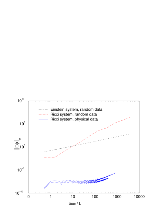
FIG. 2.: A log-log plot of the $\ell_{\infty}$ norm of the Hamiltonian constraint as a function of time for a Stage 3 test of the evolution-boundary algorithm of the Einstein system and of the Ricci system with constrained boundary. The upper two curves correspond to stability tests (random data), while the lower two curves indicate performance tests (physical data).

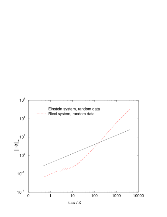
FIG. 3.: A log-log plot of the $\ell_{\infty}$ norm of the Hamiltonian constraint as a function of time for a Stage 4 test of the evolution-boundary algorithm of the Einstein system and the Ricci system with constrained boundary.

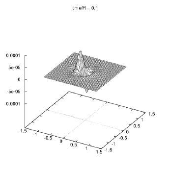
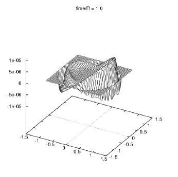
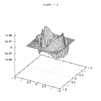
FIG. 4.: Stage IV evolution of an outgoing solution using the reduced harmonic Ricci system with a constrained spherical boundary. The plots show the metric field $h^{yt}$ at $x=0$, for $t/R=0.1$ (top), $t/R=1.0$ (middle) and $t/R=1.5$ (bottom). In the bottom plot, the field has decayed by two orders of magnitude.

REFERENCES

- [1] H. Friedrich and G. Nagy, Commun. Math. Phys., 201, 619 (1999).
- [2] T. DeDonder, La Gravique Einsteinienne (Gauthier-Villars, Paris, 1921).
- [3] C. Lanczos, Phys. Z., 23, 537 (1922).
- [4] Y. Foures-Bruhat, Acta. Math., 88, 141 (1955).
- [5] H. Friedrich and A. Rendall, in Einstein’s Equations and Their Physical Implications, edited by B. Schmidt (Springer, New York, 2000).
- [6] C. Bona, Int. Series of Num. Math., 129, 105 (1999).
- [7] H. Friedrich, Commun. Math. Phys., 107, 587 (1985).
- [8] “Harmonic coordinate method for simulating generic singularities”, D. Garfinkle, gr-qc/0110013.
- [9] B. Szilágyi, R. Gómez, N. T. Bishop and J. Winicour, Phys. Rev. D, 62, 104006 (2000).
- [10] R. Arnowitt, S. Deser and C. Misner, in Gravitation: An Introduction to Current Research, ed. L. Witten (New York, Wiley, 1962).
- [11] Y. Choquet-Bruhat, in Gravitation: An Introduction to Current Research, ed. L. Witten (New York, Wiley, 1962).
- [12] R. M. Wald, General Relativity, (University of Chicago Press, Chicago,1984).
- [13] J. Rauch, Trans. Am. Math. Soc., 291, 167 (1985).
- [14] B. Gustafsson, H.-O. Kreiss and J. Oliger, “Time Dependent Problems and Difference Methods” (Wiley, New York, 1995).
- [15] J. M. Stewart Class. Quantum Grav., 15, 2865 (1998).
- [16] B. Szilágyi, Cauchy-Characteristic Matching in General Relativity, Ph.D. thesis, University of Pittsburgh (2000), gr-qc/0006091.