I would like to thank my supervisors Dr.R.Percacci for his continued support throughout the period of my study, and Prof.R.Sorkin with whom I have worked closely in the final year of my Ph.D, and who provided the main focus of my thesis.I should not forget Prof.J.Starthdee who was not just my diploma course dissertation supervisor but has always been a sourse of inspiration and encouragement.

I would like also to thank the General Relativity Group of Syracuse University for their kind hospitality at the initial stage of the work. It is also pleasure to thank Abdus Salam Center for Theoretical Physics, especially the High Energy Group and all the professors of H.E.P Diploma course 94-95. I don’t forget all my friends and brothers from ICTP, SISSA and Syracuse University, however the space left in this page is too small to mention all the names…. To my parents, my sister and my son, in the memory of Marouan.

Abstract

The Causal Set hypothesis asserts that spacetime, ultimately, is discrete and its underlying structure is that of a locally finite partial ordered set, and macroscopic causality reflects a deeper notion of order in terms of which all the geometrical structure of spacetime must find their ultimate expression. After reviewing the main aspects of Causal Sets Kinematics, and the recently developed Stochastic Dynamics. We concentrate on possible implications in the fields of cosmology and black holes. In the context of black hole, we propose a possible interpretation of the entropy as the number of links crossing the horizon.

Introduction

General relativity (G.R) and quantum mechanics (Q.M) are the two major pieces of our understanding of the physical world. These two theories are consistent with the facts they were created to explain. Quantum Mechanics or Standard Model of particle physics has found a dramatic empirical success, showing that quantum field theory (QFT) is capable of describing all accessible fundamental physics, or at least all the non-gravitational physics. General relativity is capable of describing all the large scale phenomena, and it is, perhaps, the best tested theory ever constructed in the history of physics. These two theories offer us the best confirmed set of fundamental rules. More importantly, there aren’t today experimental facts that openly challenge or escape this set of fundamental laws. On the down side, when we try to combine these two elements we run into apparently insurmountable technical and conceptual problems [1, 2, 3] .

With the exception of the cosmological constant problem, the need for combining the two theories cannot be addressed directly to any observed property of the world that can interplay general relativity and quantum theory. This stems from the fact that Planck length -defined using dimensional analysis as:$=(G\hbar/c^{3})^{1/2}$- has an extremely small value, which is well beyond the range of any foreseeable laboratory-based experiments. And it seems that the only physical regime where the effects of quantum gravity might be studied directly is in the immediate post big-bang era of the universe which is not the easiest thing to probe experimentally.

The motivations for studying quantum gravity or looking for a more fundamental structure for space-time are more of internal nature:for example, the search for mathematical consistency, the desire for a unified theory of all forces, or the implementation of various quasi-philosophical views on the nature of space and time e.g why do we live in 4-d spacetime? why is the universe so big….etc [2]. The theoretical consequences of these two theories, and most importantly the discovery of the quantum induced radiation by black hole, were major reasons for studying quantum gravity to understand the end state of gravitational collapse and the so-called information loss puzzle that accompanies it, and the origin of the black hole thermodynamics. On the other hand and interestingly, the conceptual and interpretive problems that confront the quantization of gravity in any standard way, are the same as those that have plagued the foundations of quantum mechanics in general, ranging from the measurement problem to the meaning of probability.

All this has led to the belief that a consistent theory that would combine quantum mechanics and G.R may require a radical revision of our most fundamental concept of spacetime and substance [1, 2].

Over the last three decades the subject of quantum gravity witnessed much progress along different lines and the emergence of many ideas that range from very conservative to very radical ones . It is not, of course, the aim of this introduction to mention all these developments, but it is fair to say that String Theory stands as the most developed the idea and the one that attracted most [3, 4].The recent understanding of its non-perturbative aspects, makes it the most promising candidate for unified theory of all forces, hence providing a quantum theory of gravity [4]. This of course by no means leaves no room for other approaches. At the end there is no reason to expect that different approaches are necessarily exclusive. On the other hand, it is also fair to say that none of the present approaches has provided a satisfactory answer to any of the long standing questions, for which those theories were first created [3].

One of the approaches to quantum gravity that witnessed a considerable progress and has started getting more attention, and gaining popularity is the causal set approach.

The causal set hypothesis asserts that space time , ultimately, is discrete and that its underlying structure is that of a locally finite, partial ordered set which continue to make sense even when the standard geometrical picture ceases to do so.

The causal set idea was first considered in the quantum gravity context first by t’Hooft [5], however without being developed to any extent, Meyrheim considered independently the same idea (may be from a pure geometrical point view) and developed what on may call Statistical Geometry [6] , although the line of development of Meyrheim overlaps with many aspects of the Kinematics of the causal set the underlying idea is dynamically different from the causal set one, and the issues with which the causal set set is mainly concerned were not dealt with.

It was not until the late 80’s that the idea of causal set was taken up seriously and studied systematically as an approach to quantum gravity.

The causal set approach, and to many respect, can be said to be less developed compared with other approaches , as String theory,or Loop Gravity, it experienced a considerable progress on its kinematic aspects and a significant advance has recently been made along the dynamical front.

The basic motivational observation behind the causal set idea range from physical-conceptual, and technical, to pure mathematical ones [1, 10, 9, 8].

Physical Motivations

The main reasons that make people find an underlying discreteness of spacetime more natural than the persistence of a continuum down to arbitrarily small sizes and short time, can be summarized in what Sorkin has called the three (or four) infinities [11].

The first one is the infinity(ies) that plague all renormalizable quantum field theories, when one tries to make prediction. These infinities can be dealt via Renormalization , however this procedure has been for many workers not satisfactory, and only an indication that something is going wrong at some energy scale, the non-perturbative study of $\phi^{4}$ theory which is an essential ingredient of the standard model has shown (although not in an absolutely conclusive way [12]) that this theory can’t be consistent above some energy scale unless it is trivial, the same results are believed to hold for any theory which is not asymptotically free, Abelian gauge theory is an example, in this sense Standard Model can’t have any predictive power above some energy scale . On the other hand the Renormalization procedure which enable us to make predictions, fails to give an unambiguous results when gravity is included ( not necessary quantized), unless the metric of the spacetime background is static or stationary, but there is no reason why a semi-classical metric should have this property [2].

The second type of infinity is the one that ruin any procedure to quantize gravity, and in this case one cannot apply the renormalization procedure that works for what are usually called renormalizable theories, and here one is not able to make any prediction at all. However it should be noted that when gravity is understood as an effective theory with cutoff around the Planck scale one is able to do a quantum realistic calculation and make prediction [15, 16, 14]

The third infinity is ,maybe, less appreciated than the others, and often overlooked, this infinity occurs whenever one tries to account for the for contribution to the black hole entropy, which can not be excluded on any physical ground, unless a short distance cutoff is introduced those contribution are inevitably infinite. And it seems that this infinity is closely related to the infinity met when one tries to quantize gravity [40].

The fourth infinity is singularities in classical general relativity that are inevitable in many physically reasonable contexts, inside the black hole or in the big-bang, in the singularities our laws break down and one fails to make any prediction.

Above these infinities there are more reasons that point towards discreteness . The fact that the we have a dimensional scale, the Planck scale, can be understood as an evidence for discreteness underlying the fundamental structure of ”spacetime”, this scale can’t emerge from a continuous picture ”smooth manifold” of spacetime, (at least with relatively simple topology), and would turn out be zero or infinity. The recent development of string theory and the recent calculation of loop gravity, are all pointing towards some kind of discreteness, or fuzziness of spacetime. The uncertainty principle combine with G.R connection between mass and spacetime -curvature in such a way that it is impossible to measure the metric on a sub-Planckian scale, without the apparatus collapsing into black, leading to sort of fuzziness in the space, and the continuum geometric picture of spacetime ceases to make sense.

Mathematical Motivations

Here I give a brief account for some known, although insufficiently appreciated, pure mathematical results showing how the classical spacetime’s causal structure comes very close to determining its entire geometry , i.e Topology, differential structure, and the conformal metric.Those results once combined with the above physical motivations seem to lead naturally to the Causal Set picture.

In general relativity a space time is usually assumed to be a 4-d connected $C^{\infty}$ Hausdorff manifold $M$ endowed with a Lorentzian metric $g$ and time orientation. Once the time orientation is given one can speak about future and past.

A point $x$ is said to be in the causal future (past) of a point $y$ and we write $x\in J^{+}(y)$ $(x\in J^{-}(y))$ if there is a future (past) directed causal curve (Time like or null) from $x$ to $y$.

Other basic definition is of the chronological future (past) of a point $x$, denoted by $I^{+}(x)$ ($I^{-}(x)$), defined as the set of points which can be connected to $x$ by future (past) directed timelike curve.

The causal relations defined above can be used to put a topology on $M$ called the $Alexandroff$ $topology$, this is the topology in which a set is defined to be open if and only if it is the union of one or more sets of the form $I^{+}(x)\cap I^{-}(y),x,y\in M$. As $I^{+}(x)\cap I^{-}(y)$ is open in the manifold topology , any set which is open in the Alexandroff topology will be open in the manifold topology, the converse is not necessarily true. However if the strong causality condition holds for $M$, the Alexandroff topology coincides with the manifold topology of $M$, since $M$ can be covered by local causal neighborhoods as one can find about any point $x\in M$ a local causal neighborhood.This means that if the strong causality holds, one can determine the topological structure of the spacetime by observation of causal relationships, stated otherwise, the topology of spacetime is already coded in its causal structure.

It is a standard result that by knowing which points can communicate with a given point $p$ one can determine the null cone in the tangent space of $p$ .Once the null cone is known, the metric can be determined up to conformal factor.

The above statements can be strengthed (relaxing the strong causality condition) and made more precise by the two following theorems .

$Theorem$[17] : Let $(M_{1},g_{1})$ and $(M_{2},g_{2})$ be spacetimes and $f:M_{1}\rightarrow M_{2}$ a homeomorphism where both $f$ and $f^{-1}$ preserve future (past) directed continuous null geodesics.Then $f$ is a smooth conformal isometry.

$Theorem$[18] : Suppose $(M_{1},g)$ and $(M_{2},g)$ are past and future distinguishing spacetimes and $f:M_{1}\rightarrow M_{2}$ is a causal isomorphism.Then $f$ is a homeomorphism .

Now the second theorem asserts that tow spacetimes having the same causal structure (There is a causal isomorphism between them), and both future and past distinguishing , then they must be homeomorphic, hence topologically equivalent, and this isomorphism with its inverse can be shown to preserve future (past) directed continuous curves which in turn would imply that the isomorphism, being also a homeomorphism, preserve null geodesics, and by the first theorem must be a conformal smooth isometry. This result is of great interest in its own right since [18, 7], the bottom line of the above assertions is that the two spacetimes have the same conformal structure. So given a spacetime obeying suitable smoothness and causality conditions one can retain from all its structure only the information embodied in the causal order .Then one can recover from the causal order not only the topology of the spacetime but also its differential structure, and the conformal metric.

Now what is a causal order? It is simply a partial ordering between points in the spacetime, and the above construction can be turned ”on its head” with the partial ordering relation construed as primitive, and in fact it is natural to guess that in reality one should derive from the causal order the metric rather than the other way around. The problem with this new construction is the lack of information to determine the conformal factor of the metric.In other words, we get from the causal relations the metric, but without its associated volume. There seems to be no way to over come this problem within the context of the continuous space time (in fact, this is all what can hope for since all conformally equivalent Lorentz metric on a manifold induce the same causal structure), but as we discussed in the physical motivations, there are many reasons to doubt that spacetime is truly continuous. If instead we postulate that a finite volume of spacetime contains (a large ) but finite number of points (events or space time atoms) then we can -as Riemann suggested- measure the volume of a region in spacetime by merely counting the number of points it contains, provided some density set by some fundamental scale .

So by putting the conceptual and the mathematical motivations together we arrive naturally to a new ”substance” (Structure) underlying spacetime is what Riemann might have called an ”ordered discrete manifold” but we will call ”causal set ” or what is known in discrete mathematics as Partially Ordered Sets ( Posets). In this view the volume is a number, and macroscopic causality reflects a deeper notion of order in terms of which all the geometrical structure of spacetime must find their ultimate expression.

At the end of this section it is intriguing to note, assuming the that this proposal is step in the right road, how the ultimate (fundamental) rules of space-time, may find their ultimate expression in such a simple mathematical object as the Partially Ordered Sets.

This thesis is organized as follow, in the first chapter we review the Kinematic aspects of the causal set that was developed by Sorkin and Bombelli, Daughton, Meyer including some relevant recent results. In the second chapter, after reviewing the dynamical aspects including some old proposals and the recently developed stochastic dynamics, we outline possible cosmological implications of this dynamics. The third chapter after brief review of the main aspects of Black Hole thermodynamics and the notion of Entanglement Entropy , we propose a possible interpretation of the black hole entropy and we interpret it on the light of entanglement entropy and information theory and we conclude by some remarks on other possible interpretions of the result obtained.

In appendix A a technique is developed for calculating volumes needed to ensure some causality conditions in 4-d flat spacetime.

Appendix B contains a detail account for the derivation of the results that appeared in Chapter 3.

Chapter 1 Kinematics Of Causal Sets

In this chapter, I review the basic definitions and terminology of posets relevant for causal set theory, focusing mainly on the physical aspects which have been developed by Bombelli, Meyer, Sorkin and Daughton [7, 8, 9, 23].

As in any new developed physical theory, the first step towards a complete understanding of its physical insight is to understand the Kinematics. Here by the Kinematics of causal sets we mean the study of the general structure of causal sets, more precisely to see how to make contact between causets and spacetime. As it turned out, concepts such as length, topology, and dimension make little sense for generic causal set; so it is necessary to understand in what circumstance they do emerge in a purely causal manner.

In order to be able to address such question and many other physically relevant questions we will encounter later on, new mathematical concepts had to be introduced, above the already existing ones in the theory of partial ordered sets which in itself forms a category .

1.1 Basic definitions and New concepts

A partially ordered set (or a poset for short) ${\cal P}$ is a set endowed with a relation $\prec$ satisfying the following axioms:

(1) reflexive : $\forall$ $p$ $\in$ ${\cal P}$ , $p$ $\prec$ $p$

(2) transitive: $\forall$ $p,q,r$ $\in{\cal P}$ , $p$ $\prec$ $q$ $\prec$ $r$ $\Rightarrow$ $p$ $\prec$ $r$;

(3) antisymmetric : $\forall$ $p,q$ $\in$ $P$ , $p$ $\prec$ $q$ and $q$ $\prec$ $p$ $\Rightarrow$ $p$ $=$ $q$.

Notice here that the refelxivity axiom is a matter of convention and we could have used instead the irreflexive convention

If $p\prec q$ , $p$ ($q$) is said to be in the past (future) of $q$ ($p$).

The future (past) of an element $p$ is the set of all element which are in the future (past) of $p$.

An interval (Alexandrov set) $J(p,q)$ defined by two elements $p,q$, with $p\prec q$, is the intersection of the future of $p$ with the past of $q$:

$$J(p,q):=\{r\mid p\prec r\prec q\}.$$ (1.1)

An interval is a special case of induced subposet, a subset ${\cal P}^{\prime}\subset{\cal P}$ in which two elements are related, $p\prec q$, iff they are related in ${\cal P}$.

An element is called maximal (minimal) if there is no elements to its future (past).

A $chain$ is a subset of $P$ in which any two elements are related ( a totally or linearly ordered subset).

A $locally$ $finite$ poset is a poset ${\cal P}$ such that all the Alexondrov sets are finite (have finite cardinality) .

A useful concept for the description of locally finite posets is the $link$, if the interval $J(p,q)$ contains no element except $p$ and $q$ themselves, and we say there is a link between $p$ and $q$, or $q$ cover $p$ and we write $p\prec\cdot q$, this notion is similar to that of the nearest neighbor for lattices embedded in manifold with positive-definite metrics. It should be remarked that, for a general poset, there is no metric meaning associated with this notion of closeness in the partial order, although in some cases it is related to a notion of closeness in a Lorentzian metric.

The knowledge of all links is equivalent to knowledge of all relations among elements: $p\prec q$ iff there are elements $q_{1},q_{2},,......q_{n}$ such that $p\prec q_{1}\prec\cdot q_{2}\prec\cdot,,.....\prec\cdot q_{n}\prec\cdot q$.

A $Path$ between $p$ and $q$ is a $maximal$ $chain$ between these elements, i.e, a chain made of links, like $p\prec q_{1}\prec.q_{2}\prec\cdot,,,.....\prec\cdot q_{n}\prec\cdot q$.Two paths between $p$ and $q$ need not have the same $length$ (number of links), and we will call ”maximal path” one with the maximum length.

A connected poset is one for which there is at least one path which can be followed to go ”continuously” from any given element to any other element allowing backward.

A $null$ $path$ is path which is also the interval formed by its endpoints (in Minkowski space, the only points causally related to two null-related points are those on the null geodesic joining them).

An $antichain$ is any subset of a poset ${\cal P}$ in which no two elements are related; whereas a maximal antichain is an antichain such that no further element can be added to it.

The $width$ of a poset is the size of the largest antichain, and the $height$ is the length of the longest path.

A $join-independent$ subset of ${\cal P}$ is a subposet ${\cal P^{\prime}}$ of ${\cal P}$ such that, for every $p^{\prime}\in{\cal P^{\prime}}$, there is a $p\in P$ , with $p^{\prime}\not\prec p$, but $p$ is to the future of every other element of ${\cal P^{\prime}}$ (such a ${\cal P^{\prime}}$ is always an antichain). The $breadth$ of ${\cal P}$ is the size of its largest join-independent subset.

A $loop$ is a pair of paths between two elements, which do not meet except at their endpoints.

$EXAMPLES$

(a) the totally , or linearly , ordered set with $n$ elements,

$${\cal P}^{l}_{N}=:\{a_{i};i=1,...N|a_{i}\prec a_{i+1};i=1,...,N-1\};$$

(b) the ”fence” poset of size $2N$,

$${\cal P}^{f}_{2N}=:\{a_{i},b_{i};i=1,...N|a_{i}\prec b_{i},\forall i;a_{i}\prec b_{i-1}\};$$

(c) the set $2^{[n]}$ of all subsets of $[n]$ ( a set of n-elements) ordered by inclusion i.e., $A\prec B$ $\Longleftrightarrow$ $A\subset B$ as sets; this is called the binomial poset $B_{n}$ .The binomial posets are of a particular importance, because of the results known about them, and the possibility of realizing any poset as a subposet of some binomial poset .

A $Hasse$ $diagram$ for a poset is a one-to-one mapping from the poset to the two dimensional Euclidean space such that each element is mapped to a point and a link to a line, with a point $p$ is placed above $q$ if $q\prec p$; Fig (1.1) illustrates this definition for the following poset.

$$S=\{a,b,c,d,e,f\}$$

With the partial order :

$$a\prec\{b,c,d,e,f\};b\prec\{d,e\};c\prec\{d,e,f\};d\prec\{e\}.$$

Figure 1.1: Hasse diagram for the poset $S$ defined below.

Given the above examples of partial ordered sets it is natural to ask how many different posets one can construct with $n$ elements. This question turns out to be an unsolved problem in combinatorics for a generic $n$: in fact the answer is known only for $n<14$ and for large $n$ and asymptotic formula is available.

$$D_{n}\approx C2^{\frac{n^{2}+6n}{4}}e^{n}n^{-n-1}$$ (1.2)

where $D_{n}$ being the number of different posets and $C$ is a number of order one.

Having introduced the above terminology we are now ready to give a precise definition of our central object.

A Causal set (or causet for short) is a locally finite connected poset.

From here on we will only be interested in causets.

1.2 Realizations of posets

It is often useful to think of a poset in terms of some realization of it, by realization of a poset we mean a mapping of poset to another mathematical object preserving all the order existing in the poset. Here one should bear in mind that our aim is not to look for applications of posets or to find their realizations, the realization serves only as a mathematical tool to gain more insight to the posets structures through the known mathematical structure of the realization, and at the end we should be able to formulate the physics of causal set without any reference to their realization. However as a first step towards the understanding of the laws (Kinematics and Dynamics) of causal sets, we will often think of a poset ${\cal P}$ as realized in terms of points in a Lorentzian manifold $({\cal M},g)$ this realization we will call a conformal realization of ${\cal P}$. In a physical term, since the low energy physics of the causal set dynamics, (or whatever theory which is taken to be a candidate for the ”quantum” theory of gravity) must give us the the Lorentzian geometry , and as well known the low energy physics may constraint very much the high energy physics, so it is natural to start by understanding the causal realization.

A $Conformal$ $realization$ is defined as follow,

let ${\cal P}$ be a poset and $({\cal M},g)$ a Lorentzian spacetime with metric $g$, a causal realization is a map $f:{\cal P}\rightarrow M$ with $f(p)\in J^{-}(f(q))$ iff $p\prec q$.

Another useful and common realization is the linear realization in which elements of ${\cal P}$ are mapped to points in $\mathop{\mbox{Re}}^{n}$ for some $n$ and the ordering is reproduced by the partial ordering induced by the coordinates: $f:{\cal P}\rightarrow\mathop{\mbox{Re}}^{n}$, with $f^{i}(p)\leq f^{i}(q)$, $\forall i$ iff $p\prec q$.

1.3 Causal sets and differentiable manifolds

Recall that our a proposal is to take this causal set as the matter underlying spacetime and as mentioned in the introduction our large scale perception of space time is that of a continuous manifold . The explanation of the emergence of this structure is by now one of the (if not the most ) most fundamental questions in theoretical physics. Answering this question in the casual set approach would need a full understanding of the dynamics of causal set, but what has been done in the context of causal set is to try to address more moderate questions, as for instance, to what extent the elementary structure of causets could give rise to Lorentzian Manifold in some suitable approximation? and others questions we will encounter later on.

I first start by giving some definitions which are used in formulating such questions in a causal set terms.

Definition

A causal realization of a poset ${\cal P}$ in a spacetime $({\cal M},g)$ is said to be a faithful embedding if:

(1) The embedded points are distributed uniformly with respect to the volume form on $({\cal M},g)$ with density $\varrho$ and

(2) The characteristic scale over which the continuous geometry varies appreciably is everywhere much greater than spacing between the embedded points.

And $({\cal M},g)$ is said to be associated to ${\cal P}$.

Let me now try to explain and motivate the above definition.

By uniformly distributed points we mean if one take an arbitrary Alexondrov neighborhood of size $V$ in ${\cal M}$, the number of embedded points in it is $\varrho V$, within the Poisson-type fluctuation which could be expected from a random ”sprinkling” of points, so the probability distribution for having $n$ points in the neighborhood is a given by Poisson distribution ,

$${\cal P}(n)=\frac{(\varrho V)^{n}e^{-\varrho V}}{n!}$$ (1.3)

that is to say that the image of the causal set looks as an outcome of stochastic process : points sprinkled uniformly and independently, i.e, there is no preferred region in the manifold as far as the density is concerned, the probability of finding a point in region of finite volume depends only on the volume of the region.

The second condition can be taken simply to require that each embedded point have a suitable neighborhood, which is approximately flat, see [Bombelli [8] for more discussion of this point and possible implications].

The above definition for a faithful embedding seems to be the only one consistent with our intuition and general covariance for a manifold to be a continuum approximation to a causal set, this can be seen as follow.

Two elements related in the causal set their image will be causally related; unrelated elements will have a space like related images. The order relation in the causal corresponds to the time orientation in the manifold.

If two elements are linked in the casual set then their images under an embedding will be nearest neighbors :the Alexandrov neighborhood they determine will contain the image of no other element in the causal set.

A chain is embedded as a sequence of causally related events -there is a causal curve passing through them.

If one tries to define reasonable non-uniform Lorentzian density in invariant sense will be forced in the end to have a uniform density everywhere, since even a small Alexandrov neighborhood can extend between ”far apart’ regions in the manifold (think for instance of Alexondrov neighborhood between two points which look approximately null in some frame, for a Minkowski spacetime) and to produce a varying density in invariant way one would have to make it uniform in all the direction, arbitrarily close to the null ones,and since the light cones of all points meet, thus we end up with the density cannot vary at all.

Note here that, this condition justifies our use of the locally finite poset, it allows to interpret the volume of a region as the number of points in it, from which one would recover the conformal factor of the metric.

The reason for imposing the second condition in the definition of faithful embedding is not just that the small lengths would not be meaningful, but also that the causal embedding with the first conditions by themselves would be far from determining a unique approximating spacetime: given any manifold with the right causal structure we would arrange the density to have a constant value by setting the conformal factor appropriately; but in doing so, we would in general introduce an unreasonable large curvature, or other small characteristic lengths, in other words the causal embedding and the uniform density condition alone would determine the continuum geometry leaving a room for arbitrary variations on small scales (spacing between embedded points or smaller) .

Now, let us go back to our starting question , i.e. To what extent a causal set determines the properties of an associated manifold?

Having given the above definitions this question can be reformulated as follow,

Given a manifold into which ${\cal P}$ can be faithfully embedded , how unique are the topology , differentiable structure and the metric?

It has been conjectured [7] , that the topology and the differentiable structure are unique, and the metric is determined up to ”small variation”.

This is the main conjecture of the causal set approach, although it is not stated in a mathematical rigorous way, there are some evidence supporting it. For instance the study of the dimension of causal sets shows (almost) the dimensionality of the associated manifold is unique, and there some arguments supporting the uniqueness of the topology and the metric.

There is a very important point to note here, the conditions imposed in the definition of the faithful embedding are very strong and in general, for a given causal set ${\cal P}$, there will be no manifold ${\cal M}$ in which ${\cal P}$ can be faithfully embedded; in fact we expect almost all the causal sets not to be faithfully embeddable anywhere, for example a crude estimation shows that only a vanishingly small fraction of causal sets with a large $N$ number of elements can be faithfully embedded in $n$ dimensional Minkowski space, i.e., $c2^{nNlog_{2}N-N^{2}/4-(3/2+log_{2}e)N+log_{2}N}$.

The last conclusion may seem at first sight a disadvantage, however this turned out to be rather an advantage as we will see in the coming sections, for the time being one is only interested to show that the causal set has a structure rich enough to imply all the geometrical properties as we attribute to continuum spacetime, in other word we are interested in the uniqueness of the continuum approximation of causal set, when it exists.

1.3.1 Dimension of causets

One of the basic aspects of the manifold is the dimension, so an obvious first question is whether there is a good way to recognize the effective continuum dimension of a causet.

In general there is no very meaningful intrinsic definition of dimension for a poset, however, it turns out that the most useful definitions of dimension for posets are those in which the dimension in some sense is not a property of the poset itself only, but of the poset and some realization of it.

First I will give two definitions, one is of the conformal dimension and the combinatorial or linear dimension, the former because of its direct physical meaning and relation to what we will call later the physical dimension, and the latter because of the many results known about it, although may turn to have a little to do with the causal one for dimensions higher than 3 as we shall see. Than I will discuss the ”Physical dimension” and the fractal dimension (statistical) which should coincide with the physical one if the causet is faithfully embeddable.

Linear dimension

As remarked earlier one of the natural realization of a poset is the linear one, and we define the linear dimension to be simply the smallest $n$ for which there exists a linear realization in $\mathop{\mbox{Re}}^{n}$.This dimension is well defined since any poset has some linear realization for some $n$, for example the binomial poset $B_{n}$ has a linear dimension $n$, and it is easy to show that any poset with no more than $n$ element can always be realized as a subposet of $B_{n}$.

Moreover many upper bounds on the linear dimension have been set:

$ldim{\cal P}\leq ldim{\cal P}^{\prime}+1$ where ${\cal P}^{\prime}$ is obtained from ${\cal P}$ by removing a single element.

$ldim{\cal P}\leq ldim({\cal P}\setminus C)+2$ where $C$ is a chain in ${\cal P}$.

$ldim{\cal P}\leq width{\cal P}$.

$ldim{\cal P}\leq(max{2,|\cal{\cal P}\setminus A|)}$ where $A$ is an antichain in ${\cal P}$.

$ldim{\cal P}\leq|{\cal P}|\setminus 2$ for $|P|\geq 4$.

$ldim{\cal P}\leq 1+width({\cal P}\setminus M)$ where ${\cal M}$ is any set of maximal or minimal elements.

$ldim{\cal P}\leq 1+2width({\cal P}\setminus A)$ where $A\not={\cal P}$ is antichain in ${\cal P}$.

Conformal dimension The conformal dimension of a causal set is the smallest $n$ for which there exists a causal embedding in $n$-dimensional Minkowski space.

This defintion is concerned only with existing of causal embedding in Minkowski space with no further condition, however, the study of the conformal dimesnion is of a particular importance since one of requirement of a faithful embedding was that each point would have suitable neighborhood which is approximately flat, this neighborhood will contain a few points and due statistical fluctuation these points need not be recognizably uniformly distributed, hence looking like a small size causet embedded in a Minkowski space time, not necessarly with uniform distribution. So suitable such subsets will contain the information on the dimension of manifold in which the causet can be embedded .

The above definition although it may seem natural, need not be defined for all posets, its definiteness lacks on some unproven (may be wrong!) conjectures, for instance if one could prove that: adding one maximal or minimal point to a causal set can increase its conformal dimension at most by one; than the conformal dimension would defined for any causet.

Note here that an equivalent version for the above statement holds for linear dimension, the One -point removal theorem, i.e, removing one point from a poset can decrease its linear dimension at most by one.

This led to the definition of special posets which encode all the information about the linear dimension.

Definition: A poset is linearly d-irreducible if it has a linear dimension $d$ and the removal of any element reduces its dimension.The $n$-irreducible poset with minimum size is called $n$-pixie.

It follows from this definition and the One-point theorem that each poset with linear dimension $d$ contains a $d$-irreducible poset. Thus the $d$-irreducible posets are $obstructions$ to have a linear dimension less than $d$ . By the one-point removal theorem the dimension of an $d$-irreducible poset is reduced by one upon the removal of any of its elements.

At this point it is natural to ask to what extent the linear dimension is related to the conformal one?

Although no proof has been provided for the one-point removal theorem in the case of conformal dimension one might try to define conformally irreducible causal set, along a similar line and obtain similar results when the causal embedding exists, as for instance, a causal set with a causal dimension $d$ must contain a $d$-irreducible causal set.This follow from the fact that a weaker version of One-point removal theorem holds, since if a causal set were embeddable in $d$-dim Minkowski space we know that by removing elements we would not increase the dimension , so by removing elements whose removal does not reduce the conformal dimension, and when no such elements remain the causal set is $d$-irreducible. In particular we have the following theorems;

Theorem[9]:Every 3-irreducible causal set is a 3-irreducible poset and conversely.

Theorem[9]: A causal set can be embedded in two dimensional Minkowski space iff it has linear dimension at most two.

Naively one would hope that similar results hold in higher dimension but there are counter examples, a simple example is shown in fig (1.2), where a poset which can only embedded linearly in four dimension or bigger but it can be embedded in three dimensional Minkowski space[9].

Figure 1.2: This diagram shows the explicit causal embedding in 3-dimensional Minkowski spacetime of a poset having the above Hasse diagram, via its realization in terms of balls in 2-dimension

Now it is natural question to ask if there exist at all causets which can be only in higher dimension $d\geq 4$, in other words, are there causets capable of characterizing arbitrarily great spacetime dimension?(Are there $d$-irreducible causets with $d\geq 4$?)

First it has been proven by Meyer [9], that if a binomial $B_{n}$ poset with $n\geq 6$ can be causally embedded in a Minkowski space with dimension $d$, than $d$ is at least as large as some number, more precisely we have the following theorem .

Theorem:The conformal dimension of binomial poset $B_{n}$ is at least as large as the minimal $d$ satisfying :

$${n\choose d}\geq\sum_{i=d+1}^{n}{n\choose i}.$$

In some sense this theorem doesn’t prove any thing concerning the question we asked, since it could be (and it seems likely to be [see citespro1 and references therein]) that there is no causal embedding at all for such a binomial posets, however , it has been shown Brightwell and Winkler [20], that the poset $P_{n}$ made by retaining from the binomial poset $B_{n}$ only the relations embodied in the following rule:

$$p_{1}\prec p_{2}\rightarrow p_{1}\subseteq p_{2}\qquad\mbox{and}\qquad|p_{1}|=1\qquad\mbox{or}\qquad|p_{2}|=n-1$$

can be embedded in $n$ dimensional Minkowski space (or higher of course). and not in $n-1$ dimensional Minkowski space.

The last result shows that irreducible causet of arbitrary dimension do exist, they can be obtained simply by removing points from the above defined family of causets until they become embeddable in lower dimension, their dimension may decrease by two or more upon the removal of one element, however.

At the end of this section it may seem surprising that with our intuitive definition of the conformal dimension we have not even able to proof its existence (Definiteness) of causal sets, moreover it is very possible that the above conjectures may turn out to be wrong, and only some special posets have a definite conformal dimension, in fact it has been suggested [11] that , the binomial posets ($n\geq 6$) may not embeddable in any dimension (however, if one allows for highly curved spacetime the causal embedding could be possible [23]). The subject of causal embedding of posets is still under investigation [23]. Finding the characteristic causets similar to the family we mentioned above (or at least their general properties) would, in fact, shed a light on the construction of the dynamics of causal sets.

1.3.2 The physical dimension and fractal dimension

Recall that our starting point was that a faithful embedding would give us almost all the geometrical information about the associated manifold and in particular the dimension, however as remarked earlier we don’t expect all posets to have a faithful embedding -actually almost none will have- and any definition of the dimension based on the dimension of the manifold in which the causal set can be faithfully embedded would be far from giving a well defined mathematical entity.A more practical definition of dimension has been proposed by Meyer , Bombelli, [8, 9] and is called fractal dimension or Myrheim-Meyer dimension, which should reduce to the the physical dimension defined to be the dimension of the associated manifold when it exists.

The fractal dimension is statistical in character and here I give a very brief sketch of it.

The fractal dimension is defined in a $quasilocal$ way, being associated with different regions in the causal set rather than the whole set. What one merely does here is to take an interval (small enough) and count the number of elements it contains , and define a quantity using the interval for which theoretical( statistical) dependence on the volume of the interval and the dimension is known for causet embedded in Minkowski space. Then by inverting the relation governing the dependence one can in principle obtain an effective dimensionality for this interval. Now, if one can cover the a large region of the causal set by intervals all roughly with same size, and all yielding almost the same result for the dimension one can associate this dimension to the casual set, however if different regions gave different results one would conclude that we were dealing with a set which is not faithfully embeddable. In general we expect the resulting dimensions to agree, if the causal set we consider is faithfully embeddable in a curved spacetime, provided they are derived from intervals small enough that the result is not significantly affected by curvature, however, these methods are of course subjected to statistical fluctuations which should be small for large intervals, but it may happen that the interval with the right size to offset statistical fluctuation becomes large not to be negligible with respect to the radius of curvature of space-time.The above mentioned limitation on the applicability of these methods may be turned to an advantage and, in fact, used to estimate the curvature[9, 8]

The following example illustrate how the idea of fractal dimension works.

For $N$ points sprinkled uniformly in an interval in Minkowski spacetime, the expected number of elements to the future of a point $x$ is $V(J^{+}\cap A)$, and the expected number of relations in $A$ is

$$<N_{rel}>=\int_{A}V(J^{+}\cap A)dV=V(A)^{2}f(n)$$

where

$$f(n)=\frac{\Gamma(n+1)\Gamma(n/2)}{4\Gamma(3n/2)}$$

Now, since the expected number of elements in $A$ is $<N(A)>=V(A)$ , we may count the number of elements to approximate the volume , count the number of relations to the right hand side of the above equation, plug them in and invert $f(n)$ to obtain an approximation for the dimension of the Minkowski space in which the causet can be faithfully embedded.

Numerical simulations show that the Hausdorff dimension can be effectively computed , and numerical results are available for points sprinkled in 2 ,3 ,4 Minkowski space and de Sitter space, with the computed dimension converging rapidly to the true one as the number of sprinkled points becomes larger, the result being in general agreement with error allowed by statistical fluctuation [9]. An interesting result being for the case of ”Kaluza -Klein cylinder” of 1+1-dimension. In this example one sees clearly how the effective dimension falls gradually from 2 down to 1 as the size of the interval in question increases , showing how coarse-graining can induce ”dimensional reduction”, and how such scale-dependent dimensionality or more generally topology becomes a perfectly well-defined concept in the context of causal set, more about this later.

1.3.3 More topological information

In the previous section we have revealed that the causal set contain dimensionality information, now what about the more general question,i.e, Does a causal set ${\cal P}$ encode the topology of the manifold it is sprinkled in?

This aspect of the Kinematics of causal set is by far the less developed, at least compared to the dimension. There have been many suggestions and interesting ideas without being concretized, however.

Here I sketch very briefly some suggestive ideas of how one can hope to extract the ”germs” of a notion of incidence, around which the topology is essentially built, from the causal set. The general idea is to try to construct a finite topological space, or a finite simplicial complex, or more generally cell complex, independently of any mapping between the causet and manifolds ,i.e,depending only on the structure of the causet itself.

In general the topological spaces constructed from the causet have some topological properties which are not related to the topological spaces we may hope to get, as for instance, if one defines a simplicial complex from ${\cal P}$ by associating with every element a vertex, and with every chain of length $k$ a $k$-simplex, whose vertices are those associated with the $k+1$ elements in the chain.Thus, if a j-chain is contained in a $k$-chain $(j<k)$ then the corresponding $j$-simplex is a face of the $k$-simplex.The resulting simplicial complex is called the order complex of ${\cal P}$ [8] and its dimension is the length of the longest chain and hence the height of the causal set, and this dimension is of course not related to the dimension of the topological space we were hoping to get.

On the other hand given a causal set sprinkled in a manifold ${\cal M}$, we can define a cover of ${\cal M}$ by choosing a collection of Alexandrov neighborhood which cover it.Now a cover of a topological space defines a simplicial complex, and one way to define is to construct the $nerve$ of the open cover, and we might hope that the nerve of an appropriately constructed cover of ${\cal M}$ by Alexondrov neighborhood would be a simplicial complex with the right topology to be a triangulation of $\cal M$.The problem with this construction is that we don’t know if such a good cover always exists in term of Alexondrov neighborhoods whose intersection properties are expressible just in term of $\cal{\cal P}$.

A more direct way to construct a simplicial complex using the sprinkled causal set, is try to find an Lorentz analogue of the known Dirichlet-Voronoi construction for random lattice in Euclidean space, which yields a simplicial complex and an associated dual cell complex. Or more general construction like the one used by Lee [19] for Euclidean spaces (based on arbitrary convex regions which differ from each other by a translation and/or dilatation, and which is equivalent to Dirichlet-Voronoi when applied to spheres), this construction can be repeated for stably causal space-time with a sprinkling of points satisfying the faithful embedding conditions, using a global time function $t:M\rightarrow R$ (which is always defined for causally stable spacetimes) to isolate a collection of Alexondrov neighborhood whose endpoints belong to the same integral curve of $t^{a}:=g^{ab}\partial_{b}t$, to define simplices, and the claim is that the collection of all these simplices forms a triangulation of ${\cal M}$. see [8] for more discussion .

1.4 Coarse-graining and emergence of structures

The study of the conformal dimension, the faithful embedding, and the topology of causet has so far revealed for us the following picture.

Taking the causal set as whole may in general have no geometrical meaning , in the sense of finding a Manifold which gives a continuum approximation of the causet with all the conditions of faithful embedding full filed , and even without the requirement a faithful embedding, the causet, for instance, may acquire no well defined causal dimension.At this point we should remember that after all, our theory we seek for must enable us to arrive to the a continuum and 4-d dimensional picture of space time we experience down to the standard model scale or even to GUT’s scale.

To handle this problem one may invoke two possibilities

One possibility is that in final theory, the dynamically preferred causal sets are such that they do admit a faithful embedding, and in this way one will have solved the problem for all scale not just the large view scale, however such a picture is hard to believe for the following reasons.

Although the discussion has so far been purely kinematical we expect that the small the microscopic structure to be characterized by quantum fluctuations, or described by the interference or the superposition of many different causal sets, and we do not of course expect that, if a causal set is faithfully embeddable , any small variation of its causal structure will lead to another faithfully embeddable causet, since one could be, e.g, adding a link which creates one higher-dimensional pixie.

As a second reason, recall the success of many Kaluza-Klein type theory, in which spacetime is a manifold, but its topology at Planck scales is very different from the effective large-scale one.Such a situation could not arise from a faithful embedding of a causal set , because of our requirement on the length scales defined by the geometry unless the compactification radius is large enough [8], moreover as we will see below, if we want to put the causet theory as a candidate for providing a mechanism from which other effective fields (not only gravitational) would appear in a purely causal fundamental theory, the physically relevant causets should probably not all turn to be faithfully embeddable .

The second possibility , motivated by the above discussion, is to look for a procedure in which one can associate, in a consistent manner, a manifold to non faithfully embeddable causal set.To do this recall that our arguments indicate that the small-scale structure of causal sets which is preventing the causal set from being faithfully embeddable, so if one can smooth out these structure such that the new resulting causal set become embeddable in some manifold, this manifold would be large scale approximation of the causal set, this process in general is called the $coarse-graining$ and is in the core of statistical and quantum field theory. So far there has been no systematic way of defining a coarse-graining that would fit automatically our expectations, in fact a systematic procedure would emerge naturally from a Path Integral (Sum of histories) formulation of the dynamics of causet, such a formulation has not yet been constructed and we will postpone the discussion of some suggestive idea to the coming chapter, and try here to give some tentative ways which have been proposed in [8].

One way that one can think of is to identify elements in some set into equivalent classes, and quotienning.Doing out this equivalence relation, inducing somehow a structure among equivalence classes (In Kaluza-Klein type theories the group action defines a natural equivalence relation), however such equivalence relation must not introduce any inconsistencies in the relationships among classes of elements, a possible consistent definition is the following. Consider a collection of Alexandrov sets $A_{i}=A(p_{i},q_{i})\in{\cal P}$ having all roughly equal volume $V$ such that $\cup_{i}A_{i}={\cal P}$, and induce on it the partial order $A_{i}\prec A_{j}$ iff $p_{i}\prec p_{j}$ and $q_{j}\prec q_{j}$.This makes ${A_{i}}$ into a causal set , which we call a cover coarse-graining of ${\cal P}$, and it of course preserves only future of ${\cal P}$ with characteristic volume scale larger than $V$, however a potential problem associated with this definition is that, we might pick few $A_{i}$ ’s which are strongly boosted with respect to the others (i.e they look very long, along null directions), and would have few relations, of a kind that may make the resulting causet complicated in an undesired way.

Other way to define coarse-graining is via the notion of subset . A subset coarse-graining of a causal set ${\cal P}$ will be a ${\cal P}^{\prime}\subset{\cal P}$, with the induced partial order, satisfying a condition intended to ensure that it represents a large-scale view of ${\cal P}$, to do this we require that there exists a parameter $p\in[0,1]$ such that the fraction of all $n$-element Alexandrov sets of ${\cal P}$ which contain $k$ element of ${\cal P}^{\prime}$ is approximately ${n\choose k}p^{k}(1-p)^{n-k}$ .One can think of ${\cal P}^{\prime}$ as having been obtained by picking at random a fraction $p$ of the elements of ${\cal P}$, which makes ${\cal P}^{\prime}$ appear sprinkled with uniform density in ${\cal P}$, however with this definition we may be forcing too much randomness into ${\cal P}^{\prime}$ which may leave it (strictly speaking) as non-embeddable as ${\cal P}$ , e.g , because we are left with high-dimensional pixie somewhere

Having given the above tentative definitions for coarse-graining let us see how this process may effect the embedding of a causal set. As regards to the subset coarse-graining , if a causal set ${\cal P}$ has a conformal dimension $n$, it is easy to show that the resulting subset coarse-graining ${\cal P}^{\prime}$ will have conformal dimension $n^{\prime}\leq n$.

A similar result for the cover coarse-graining is hard to establish, however if one could choose in each set of the cover an element $r_{i}\in A_{i}$, such that $r_{i}\prec r_{j}$ iff $A_{i}\prec A_{j}$, the cover set ${A_{i}}$ would be equivalent to the subset coarse-graining ${r_{i}}$ , and the above result for the dimension would hold between ${\cal P}$ and ${A_{i}}$ , but it seems unlikely that such a points exist in general, and the situation could even be worse, since it cannot be excluded that if the cover is ”bad” in the sense described above, new higher-dimensional pixies are created by the links of the ”long” Alexondrov sets, thus increasing the dimension.

Although we have so far been unable to show that the two proposed way for coarse-gaining will wash out all unwanted feature and do not bring any new undesired features, we can give a qualitative picture for the effect of a would be systematic coarse-graining.

After some degree of coarse-graining, an initially non-embeddable causal set can acquire a well-defined physical dimension, which might however correspond to a Kaluza-Klein type manifold , and need not be the ”macroscopic” dimensionality of the causal set, obtained by further coarse-graining.

Let us now see how new effective fields (not only gravitational) may emerge from a purely causal theory through the coarse-graining mechanism.

We start by a causal set which may have no geometrical meaning , then after performing a coarse-graining , we obtain a new causet $P^{\prime}$ which is faithfully embeddable in some manifold (this manifold might have non-trivial topology , either globally, because of a possible Kaluza-Klein nature, or because of the presence of localized structures, e.g handles).

Now the new set ${\cal P}^{\prime}$ will obviously contain less information, and just by looking at ${\cal P}^{\prime}$ , one cannot tell how many extra elements there were, and how they were related.If one uses only ${\cal P}^{\prime}$ to define the dynamics (say an amplitude associated to some history ) the resulting amplitude of a given history will in general be different from the amplitude we would get using ${\cal P}$, thus leading to a different selection rules of dynamically preferred causal sets, which are the ones that determine the classical limit; and since the right amplitude should be calculated using ${\cal P}$ the extra information, or more precisely the relevant information, lost by the coarse-graining process are needed in order to continue using the same procedure with ${\cal P}^{\prime}$. The question now is to find a way to preserve the information on the original set in the coarse-grained one. It has been proposed [8] that one can do this by attaching numbers to various elements of the structure in ${\cal P}^{\prime}$, which tell us where the additional elements were and how they were linked. As an illustration, consider the following examples. If ${\cal P}^{\prime}$ is a cover coarse-gaining, to each element $p_{i}=A_{i}\in{\cal P}^{\prime}$ we can associate the number of elements in the original $A(p_{i},q_{j})\in{\cal P}$ , to each pair $A_{i},A_{j}$ the number of elements in $A(p_{i},q_{j})\cap A(p_{j},q_{j})$,…, to each collection $A_{i},A_{j},.....,A_{k}$ the number of elements in $A(p_{i},q_{j})\cap A(p_{j},q_{j})\cap...\cap A(p_{k},q_{k})$.This possibility is suggestive, since we expect the $A_{i}^{,}$ s with non-empty intersections to be nearby; in particular if we defined a simplicial complex from ${\cal P}^{\prime}$, a collection of $k$ nearby $A_{i}^{,}$ s would define a k-simplex in the complex. A possible way in which the effective fields may arise is to associate to each $k$-skeleton of the complex, which then, by its nature, would correspond to a different kind of tensor field.

To conclude this chapter let me summarize the general picture.

As regards the main conjecture of causets, if we put the various results we have obtained, we can proof the following results.

Theorem[8]: If we randomly sprinkle points in any finite region of a Minkowski space of arbitrary dimension $n$ with increasing density, after a finite number of steps we will end up with a set of points whose causal relations define a causal set $P$ with conformal dimension $n$.

Now the argument used in showing the above theorem [Bombelli [8]] uses only compact regions defined by $n$-pixies and it is natural to assume that this result continue to hold for general space-time in which all length scales defined by the metric are bounded below by some constant, so we can apply locally the above theorem.

Now using the above theorem we can go a step in proving the uniqueness of a faithful embedding.

theorem[8]:Given two faithful embedding of the same causal set, than the two associated manifold must have the same dimension.

This can be proven as follow,

Let $f:{\cal P}\rightarrow({\cal M},g)$ be a fixed faithful embedding of dimension $n$, now $f({\cal P})$ can be looked as a sprinkling in ${\cal M}$, in which case the previous theorem can be applied . Therefore, ${\cal P}$ must contain $n$-pixies as subsets. Let also $f^{\prime}:{\cal P}\rightarrow{\cal M^{\prime}}$ be other faithful embedding , since ${\cal P}$ contains $n$-pixies , $M^{\prime}$ must have at least dimension $n$. Interchanging the role of ${\cal M}$ and ${\cal M^{\prime}}$ establishes the equality between the two dimension.

It is also possible to argue that the two manifold are globally approximately isometric [8].

Notice here that even if we assume at the end that we were able to prove the uniqueness of the faithful embedding when it exists, along the above lines of argument, we would not thereby be able to characterize it for practical purposes in a pure causal set terms, and we would be only at the stage of the continuum theory of space. To understand in pure causet term we would need a constructive proof, most probably constructing simplicial complex out of causets which are a triangulation of a manifold, and, perhaps , dealing with the question of how many different causal sets give different triangulation of the same manifold.

As regard to the emergence of the picture of space time we experience today , we have seen that the causets at the fundamental level may exhibit no geometrical meaning, being purely causal, only after coarse-graining the causet may acquire continuum geometrical approximation, although not necessary a 4-dim continuum geometry we experience down to standard model scale, which may appear only after further coarse-graining , in meanwhile , some intermediate topological structures may manifest themselves in terms of geons , foam-like structure , wormholes, or internal manifold a la Kaluza -Klein, and the coarse-graining process will make fundamentally different structures appear similar. After each stage of the averaging process , the causal extra information of the original causet lost by the averaging process and not manifested as geometrical structure , may be encoded as fields living on this geometrical background.

1.5 The Issue of Locality

One of the properties that the continuum physics emerging from causet dynamics must have, is locality i.e the action contributed by causets corresponding to a given Lorentzian manifold $(M,g)$ , should turn out to be an integral of a locally defined quantity in $M$. Now, as mentioned earlier for faithful embedding in a manifold $M$, points which appear to be near neighbors in one frame will be boosted in other frames, which makes the notion of nearest neighborhood drastically different from the the one in ordinary lattices, points in Lorentzian manifold have a metric neighborhood which converges to the light cone rather to the point itself. This makes the recovery of locality rather a nontrivial task . In the case of regular Lorentz, square say (which breaks Lorentz invariance) or Euclidean lattice , locality is achieved by having only near neighbor interactions, in the continuum limit (lattice spacing going to zero) such interaction will become local.

Now, the question of locality has not yet been settled , however, as preliminary indication towards the recovery of locality was the the study ”scalar field” living in a fixed ( or ” background”) causal set (such additional degrees of freedom might or might not be necessary to incorporate ”matter”) sprinkled in two dimension [23, 24]. The main idea goes as follow , one produces several sprinklings of an Alalxondroff neighborhood in 1+1 Minkowski space.

A discretized version of the of the Laplacian operator is applied to different scalar fields (generic enough ), and then averages of the resulting actions for each field is taken. A match of the average values to the true continuum actions is the criterion under which the conclusion that locality is recoverable. The numerical results for the above program showed that the discrete version agree quite well with the continuum values. The agreement is to within a single standard error for all fields which are not rapidly varying and for which boundary terms are not expected to be present ,however if the fields are rapidly varying or some boundary terms are expected to be present, the results are decidedly not too good, and this is should in fact be expected. These results could be an indication that the locality can be recovered , regardless of the necessity of the presence of such degree of freedom to incorporate ”matter”, and thry also illustrate how locality may be emerge via a route different from that of the near neighbors.

Chapter 2 Dynamics of Causal Set

As mentioned in the introduction any procedure to quantize gravity is associated with technical and conceptual (interpretive) questions which go beyond the question of quantizing gravity in the usual sense [2, 1], and even the study of quantum field theory in fixed background addresses deep questions which are quantum in character at the end , and supported the idea that General relativity and quantum mechanics cannot coexist, however, it is widely believed that those questions will find their answer only upon a much deeper understanding of the laws which govern the dynamics of the fundamental substance of spacetime.

Now, one of the fundamental concepts of ”traditional ” dynamics is the Hamiltonian which generates the time evolution, but because time itself is discrete in the causet approach one cannot hope to write down a Hamiltonian. Indeed it is not even clear what configuration space could mean for causets, and therefore unclear what Hilbert space such a Hamiltonian could act on, in fact this approach based mainly on, Algebra of operators to be interpreted physically in terms of measurement, and Hilbert space, uses heavily the notion of spacelike Hypersurface. Apart from the fact that this approach is very questionable technically and conceptually [1] , causet does not induce any thing natural on a maximal antichain, which can then be evolved. The only available framework to work with thus appears to be that of the sum-over-histories, since it is by nature a spacetime approach, and it seems more natural to write quantum dynamical theory for causets in the sum-over-histories because of their essential covariance, as we will see below.

2.1 Old Proposals For Quantum Amplitude

In looking for the correct amplitude, there are a couple of requirements to guide us. Most obviously, the requirement that the dominant contribution must in suitable circumstances come from those causets which , upon coarse graining, give rise to the continuum geometry of classical gravity. A related requirement is that the effective action contributed by the family of all causets corresponding to a given Lorentzian manifold $({\cal M},g)$, should turn out to be dominated by the Hilbert-Einstein action.

Before I sketch some proposals let me note a very important point here, the classical dynamics for individual causets will probably not be defined at all, since the amplitude function can have no actual derivative because the causal set cannot be varied continuously , and the dynamics will not be able to be viewed as having ”arisen via quantization of some classical structure” -just as one would expect for truly fundamental theory .

To give a sum over histories formulation for causets one would associate to each causet $C$ an amplitude $A(C)$; and dynamics would be contained in the amplitude-function $A(.)$ , together with the combining rules telling how to use the amplitude to construct meaningful probabilities.

No form for the amplitude has yet been obtained , although recently Sorkin and Rideout have proposed a model for the classical stochastic dynamics of causet which may be considered as the first real step towards an understanding of the quantum dynamics which I leave its discussion to the next section, and try here to give briefly sketch of some old proposals.

These proposal are all based on associating the standard form of amplitude to the a given causet, by defining an action using one of the many structures which can be defined on causets and the amplitude is obtained by the standard way (exponentiation the action), for instance Bombelli [8] has considered the Multiloop action defined by as,

$$S_{m}(C):=lnM$$

Where $M$ is the number of distinct multiloops in $C$.

Bombelli argued that the action satisfies approximate additivity and hence one may hope to recover locality in the continuum approximation, moreover, he added an analogy between the this proposal and the 2-dimensional Ising model whose partition function can be written in a Multiloop form, although the multiloops here are not exactly the same as the one for causets. Now, near some critical temperature this 2-dimensional Ising model is known to be equivalent to local scalar field theory with definite mass, and one may hope to recover locality in a similar fashion.

Apart from these speculation this proposal has not been developed to any extent.

Another due to Geroch, is that $S(C)=2\pi Z(C)$ where $Z(C)$ is a functional on the causal set $C$ such that it is integer valued when $C$ is faithfully embeddable into a manifold and not integer valued when $C$ is not .Then

$$\sum_{c}e^{iS(C)}$$

will have constructively adding contributions for faithfully embeddable causets. Moreover, if the spectrum of $Z(C)$ is such that there exists $C^{*}$ satisfying

$$Z(C^{*})=Z(C)+\frac{1}{2}$$

for every non-embeddable $C$, then non-embeddable causets will cancel. Apart from the fact that an explicit expression for an action satisfying the above requirements has not been given, this last proposal does not fit with our expectation that not all the causets which dominate the sum-over-histories be faithfully embeddable in a manifold, however it could serve as coarse-grained dynamics.

As I remarked earlier in above proposal and many other [8, 9, 23] no calculation has been done to test the validity of the actions, because of technical difficulties due mainly to fact that one doesn’t know how to carry sums over all causets [see [23] for some proposed techniques]. To investigate the possible consequences of the causet dynamics Sorkin [11] has considered the following amplitude $A=exp(i\beta N_{rel})$, $N_{rel}$ being the number of relation as defined in the previous section. To prevent the amplitude-sums from diverging, one can take the total number of causal set elements to be a fixed integer $N$. Now, if we were to go to the corresponding ”statistical mechanics” problem by continuing $\beta$ to imaginary values, then we would be dealing with a random causal set of $N$ elements, and with probability-weight given by the ”Boltzmann factor” $exp(-\beta N_{rel})$. It happens that just this problem has been studied in connection with a certain lattice -gas model. The first result of interest is that, in the ”thermodynamic limit” $N\rightarrow\infty$ , at least two, and probably an infinite number, of phase transitions occur as $N_{rel}/N^{2}$ is varied (corresponding to varying $\beta N^{2}$ in the ”canonical ensemble”). For small values of this parameter, the most probable causal sets possess only two ”layers”, and the phase transitions mark thresholds at which successively greater numbers of layers begin to contribute. In some very general sense the causal set is thus becoming more manifold-like with each transition.

Another interesting phenomena accompanying the 2-level to 3-level phase transition is the spontaneous breaking of time-reversal symmetry. In the 2-level phase the most probable configurations look similar to their T-reversals, but the initial 3-level phase the causet of high-probability have very unequal numbers of elements in their top and bottom layers. The claim was not of course that this was the root of the cosmological time-asymmetry, but it does show the possibility that something of the sort could ultimately emerge from a better understating of causal set dynamics.

2.2 Classical Stochastic Dynamics for Causal Sets

The previous proposed quantum dynamics for causets were mainly based on some guesses and analogies with standard dynamics, and they could not be developed further due to the technical difficulties we mentioned, and it seems that a deeper understanding of what one may first mean by dynamics for causets is needed.

Recently Sorkin and Rideout have a proposed a model of defining the evolution of causet as stochastic process described in terms of the probability of forming designated causets [13]. That is, the dynamical law will be a rule which assigns probabilities to suitable classes of causets. Though the dynamics proposed there deals only with classical probabilities, can help us to get used to a relatively unfamiliar type of dynamical formulation, and would guide us towards physically suitable conditions to place on the theory.

Recall that from the sum over histories point of view, quantum mechanics is understood as a modified stochastic dynamics characterized by a non-classical probability-calculus in which alternatives interfere. In this sense the resulting theories from this dynamics should provide a relatively accessible ”half way house” to full quantum gravity .

After reviewing the main aspects of this dynamics we outline a possible implications of it. The proofs of the results quoted below and more detail can be found in [13, 22].

2.2.1 Sequential Growth

The dynamics proposed can be regarded as a process of ”cosmological accretion”. At each step of this process an element of the causal set comes into being as the ”offspring” of a definite set of the existing elements. The phenomenological passage of time is taken to be manifestation of this continuing growth of the causet. Thus, the process is not thought to be as happening ”in time” but rather as ”constituting time”, which means in a practical sense that there is no meaningful order of birth of the elements other than that implied by the order relation $\prec$. However in order to define the dynamics one ”has” to introduce an element of ”gauge” into the description of the growth process, namely the births are treated as if they happened in a definite order with respect to some fictious ”external time”, represented by a natural labeling of the elements , that is, labeling by integers $0,1,2,...$ which are compatible with causal order $\prec$. The gauge invariance is captured by the statement that the labels carry no physical meaning (this will be called ”discrete general covariance”).

It is helpful to visualize the growth of the causet in terms of paths in a poset $\cal P$ of finite causets.

Figure 2.1: The poset of finite causets

The growth will be a sort of Markov process taking place in $\cal P$. Each finite causet is one element of this poset.

A child of causet $C$ is a causet obtained by accreting a single element to the causet, and $C$ is called the parent in $\cal P$, the causets obtained in this way from $C$ will be called collectively a family. Drawing $\cal P$ as a Hasse diagram of Hasse diagrams, we get Fig (2.1).

Any natural labeling of a causet $C\in\cal P$ determines uniquely a path in $\cal P$ beginning at the empty causet and ending at $C$. As we mentioned before we want the physics to be independent of labeling, so different paths in $\cal P$ leading to the same causet should be regarded as representing the same (partial) universe, the distinction between them being ”pure gauge”.

The child formed by adjoining an element which is to the future of every element of the parent will be called the timid child. The child formed by adjoining an element which is space like to every other element will be called the gregarious child. A child which is not timid will be called a bold child.

Each parent-child relationship in $\cal P$ describes a transition $C\rightarrow C^{\prime}$, from one causet to another induced by the birth of a new element. The past of the new element will be referred as the precursor set of the transition

The set of causets with $n$ elements will be denote by ${\cal C}_{n}$, and the set of all transition from ${\cal C}_{n}$ to ${\cal C}_{n+1}$ will be called stage n.

The dynamics for the stochastic growth is defined by giving, for each $n$-element causet $C$, the transition probability from it to each of its possible children. Were not we to impose some restrictions on the transition probabilities we would be left with freedom of associating a free parameter to each possible transition, however, as we mentioned above one has to impose path independence condition in order to restore gauge invariance, the path independence condition can be stated in term of probability by requiring that, the net probability of forming any particular $n$-element causet $C$ is independent of the order of birth we attribute to its elements. Beside this condition there are other two conditions which seem natural to impose.

-Bell causality condition :The physical idea behind this condition is that events occurring in some part of a causet $C$ should be influenced only by the portion of $C$ lying to their past (hence the name bell causality). In this way, the order relation constituting $C$ will be causal in the dynamical sense.

This condition can be stated in the following way: the ratio of transition probabilities leading to two possible children of a given causet depend only on the triad consisting of the two corresponding precursor set and their union.

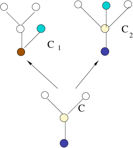
Figure 2.2: Illustrating Bell causality

Thus, let $C\rightarrow C_{1}$ designate a transition from $C\in{\cal C}_{n}$ to $C_{1}\in{\cal C}_{n+1}$, and similarly $C\rightarrow C_{2}$. Then, the Bell causality condition can be expressed as the equality of two ratios:

$$\frac{prob(C\rightarrow C_{1})}{prob(C\rightarrow C_{2})}=\frac{prob(B\rightarrow B_{1})}{prob(B\rightarrow B_{2})}$$

where $B\in{\cal C}_{m},m\leq n$, is the union of the precursor set of $C\rightarrow C_{1}$ with the precursor set of $C\rightarrow C_{2}$, $B_{1}\in{\cal C}_{m+1}$ is $B$ with an element added in the same manner as in the transition $C\rightarrow C_{1}$, and $B_{2}\in{\cal C}_{m+1}$ is $B$ with an element added in the same manner as in the transition $C\rightarrow C_{2}$ , Fig (2.2), Fig(2.3) show an example.

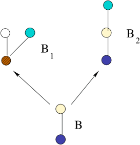
Figure 2.3: Spectators do not affect relative probability

- Markov sum rule

As with any Markov process, one must require that the sum of the full set of transition probabilities issuing from a given causet be unity. However, this depends in a subtle manner on the extent to which causets elements are regarded as ”distinguishable”. What is done here is to identify distinct transitions with distinct precursor sets of parent, which amount to treating causet elements as distinguishable.

Now, with these requirement on the dynamics one can show [13, 22] :

-The number of free parameters are reduced to at most one parameter per family

- The probability to add a completely disconnected element depends only on the cardinality of the parent causal set.

If the causets are regarded as entire universe, then a gregarious child transition corresponds to the spawning of a new, completely disconnected universe, and the probability for this to occur does not depend on the internal structure of the existing universe, but only on its size, which seems eminently reasonable.

Let $q_{n}$ be the probability of such a gregarious child transition at stage $n$ than,

- The probability $\alpha_{n}$ for an arbitrary transition from ${\cal C}_{n}$ to ${\cal C}_{n+1}$ is given by:

$$\alpha_{n}=\sum_{k=0}^{m}(-1)^{k}{m\choose k}\frac{q_{n}}{q_{\varpi-k}}$$ (2.1)

where $m$ stands for the number of maximal elements in the precursor set and $\varpi$ for the size of the entire precursor set.

The above form for the transition probability exhibits its causal nature particularly clearly: except for the overall normalization factor $q_{n}$, $\alpha_{n}$ depends only on invariants of the associated precursor set .

Now, since the $\alpha_{n}$ are classical probabilities , each must lie between 0 and 1, and this in turn would restricts the possible values of the $q_{n}$ . It turns out that it suffices to impose only one inequality per stage, more precisely it suffices that $q_{n}>0$ for all $n$ and $\alpha_{n}\geq 0$ for the timid transition from the $n$-antichain. Moreover if we define the following quantities

$$t_{n}=\sum_{k=0}^{n}(-)^{n-k}{n\choose k}\frac{1}{q_{k}}$$

than the full set of inequalities restricting the $q_{n}$ will be satisfied iff $t_{n}\geq 0$ for all $n$ with $t_{0}=1$ , since $q_{0}=1$.

One can invert the above equation and recover the $q_{n}$ in terms of the $t_{n}$,

$$\frac{1}{q_{n}}=\sum_{k=0}^{n}{n\choose k}t_{k}$$ (2.2)

Thus , the $t_{n}$ may be treated as free parameter subjected only to $t_{n}\geq 0$ and $t_{0}=1$ , if this is done, the remaining probabilities $\alpha_{n}$ can be re-expressed more simply in terms of the $t_{n}$ as.

$$\alpha_{n}=\frac{\sum_{l=m}^{\varpi}{\varpi-m\choose\varpi-l}t_{l}}{\sum_{j=0}^{n}{n\choose j}t_{j}}$$ (2.3)

Equation (2.2) implies that

$$q_{0}\equiv 1\geq q_{1}\geq q_{2}\geq q_{3}\geq....$$

So if we think of the $q_{n}$ as the basic parameters or ”coupling constants” of our sequential growth dynamics, then it is as if the universe had a free choice of one parameter at each stage of the process, however the choice is not completely free since the allowable values of $q_{n}$ at every stage are limited by the choices already made. But if we think of $t_{n}$ as the basic parameters, one has free choice at each stage. Unlike the $q_{n}$ , the $t_{n}$ cannot be identified with any dynamical transition probability. Rather they can be realized as ratios of two such probabilities, namely as the ratio $x_{n}/q_{n}$ , where $x_{n}$ is the transition probability from an antichain of $n$ elements to the timid child of that antichain.

For every labeled causet $\tilde{C}$ of size $N$, there is an associated net probability of formation $P(\tilde{C})$ which is the product of the transition probabilities $\alpha_{i}$ of the individual births described by the labeling:

$$P(C)=\displaystyle\prod_{i=0}^{N-1}\alpha_{i}$$

Which is independent of the labeling ($\alpha_{i}$ being solutions of the dynamics, satisfying the general covariance condition), this can be brought out more clearly by defining,

$$\lambda(\varpi,m)=\sum_{k=0}^{\varpi-m}{\varpi-m\choose k}t_{k+m}$$ (2.4)

Whence

$$P(\tilde{C})=\frac{\displaystyle\prod_{i=0}^{N-1}\lambda(\varpi_{i},m_{i})}{\displaystyle\prod_{j=0}^{N-1}\lambda(j,0)}=P(C)=\frac{\displaystyle\prod_{x\in C}\lambda(\varpi(x),m(x))}{\displaystyle\prod_{j=0}^{|C|-1}\lambda(j,0)}$$ (2.5)

where $\varpi(x)=|pastx|$ and $m(x)=|maximal(pastx)|$.

The net probability of arriving at particular $C\in P$ is not just $P(C)$ but

$$Prob_{N}(C)=W(C)P(C)$$

where $N=|C|$ and $W(C)$ is the total number of paths through ${\cal P}$ that arrive at $C$, each link being taken with its proper multiplicity.

Now the above expression is manifestly ”causal” and ”covariant”, however , it has no direct physical meaning in the sense of carrying a full invariant meaning. A statement like ”when the causet had a given number of element it was a chain” is itself meaningless before a certain birth order is chosen.

This, also, is an aspect of the gauge problem, but not the one that functions as a constraint on the transition probabilities that define the this dynamics. Rather it limits the physically meaningful $question$ that one can ask of the dynamics.

As an example of a truly covariant question, let us take ”Does the two-chain ever occur as partial stem of $C$?”. Recall that a partial stem is a finite subset of $C$ which contains its own past. So the above question is equivalent to asking whether or not $C$ is an antichain.

The answer to this question will be a probability, $P$, which is natural to identify as

$$P=\lim_{N\to\infty}Prob_{N}(X_{N}),$$

where $X_{N}$ is the event that ”at stage $N$”, $C$ possesses a partial stem which is a two-chain.

2.2.2 Sample Cosmologies

Although the dynamics we discussed is in its pure classical stage, it is interesting to explore and understand possible physical consequences of various choices for $t_{n}$. One of the most interesting question is of course which dynamics (choice of $t_{n}$), if any, would give us general relativity, or what are the conditions that one has to impose on the choices so that the resulting spaces from this dynamics resemble the Minkowski space or de Sitter (may be after coarse-graining).

To start with, let us consider the case of limited number of past links

$$t_{i}=0,i>n_{0}$$

With this values of $t_{i}$ it is easy to see that $\alpha_{n}$’s vanish if $m>n$. Hence, no element can be born with more than $n_{0}$ past links. This means in particular that any realistic choicer of parameters will have $t_{n}>0$ for all $n$, since an element of a causal set faithfully embeddable in Minkowski space would have an infinite number of past links.

A known example for randomly growing causet is what was called in [13] ”transitive percolation”. It is an especial simple instance of sequential growth dynamics, in which each new element forges a causal bond independently with each existing element with probability $p$, where $p\in[0,1]$ is a fixed parameter of the model. This model can be solved independently of the requirement stated for the dynamics and the transition probability $\alpha_{n}$ is given by

$$\alpha_{n}=p^{m}(1-p)^{n-\varpi}$$

Where we used the same notation as before.

With the above expression one can show that the Transitive percolation dynamics satisfy all the requirements of the general dynamics. In fact, it corresponds to the choice $t_{n}=t^{n}$, where $t=\frac{p}{1-p}$.

From a physical point of view, transitive percolation has some appealing feature, both as model for relatively small region of spacetime and as a cosmological model for spacetime as whole, where the universe cycles endlessly through phases of expansion, stasis, and contraction back down to a single element.

Other thing interesting that one learns from percolation model is that, the causets generated by the dynamics, do not at all resemble the 3-tier, generic causets of Keilman and Rothshild mentioned in the previous chapter, but rather they have the potential to reproduce a spacetime or a part of one.

Nevertheless, the dynamics of transitive percolation cannot be viable as a theory of quantum gravity, since at least two reasons, one obvious reason is that it lacks quantum interference, being stochastic only in the pure classical sense, the other reason is that the future of any element of the causet is completely independent of anything ”spacelike” to that element. Therefore, the only spacetimes which a causal set generated by transitive percolation could hope to resemble would be homogeneous, such as Minkowski or de Sitter spacetimes, but due to the periodic recollapse allude to earlier in transitive percolation, one could at best hope to reproduce a small portion of such homogeneous spacetimes.

On the other hand, in computer simulations of transitive percolation, two independent (and coarse graining invariant) dimension estimators have tended to agree. These dimension indicators vary with $n$ and one must rescale $p$ if one wishes to hold the spacetime constant. To do any better, one would scale $p$ so that it decreased with increasing $n$ [13] and reference therein. This suggests that the physically interesting choices of $t_{n}$ could be that which decrease with $n$ and by the percolation example faster than exponentially in $n$. An reasonable and simple choice could be $1/n!$, which we will discuss below.

2.2.3 Possible Cosmological Implications

It is an old idea that the universe might start, and keep bouncing, getting bigger with each bounce. The explanation of why it is so big now would then be that there have been many previous bounces. In general relativity with bouncing universe, what happens in a particular cycle is independent of what happened in earlier cycle, except insofar as they set the initial conditions for it. People have speculated that the couplings constant themselves might change, but in classical general relativity (insofar as it allows a bounce at all), that cannot occur.

Now let us pick up a particular cycle of expansion and possible contraction and call it ”the current era” for short. In the causal set context, in the current era the first event is by definition a single element $e_{0}$ which is to the future of everything not in the current era and to the past of every thing in it. Now, in percolation if we compute relative probabilities for events of the current era, it is enough to truncate the causet at $e_{0}$. This follows directly from the definition of percolation, so the dynamics in the current era is completely independent of the past eras. We will call this property locality in time.

Now what happens in the other dynamics?

First let us note the following. The probability of transitions are given by eqt(2.3)

$$\alpha_{n}=\frac{\lambda(\varpi_{n},m)}{\lambda(n,0)}$$

Where

$$\lambda(\varpi,m)=\sum_{k=0}^{\varpi-m}{\varpi-m\choose k}t_{k+m}$$

Now , recall that $\varpi$ stands for the for the precursor set defined as the past of the new elements. If we denote by $N$ the number of element in the past of $e_{0}$,

than $\lambda(\varpi,m)$ can be written as

$$\lambda(\varpi,m)=\sum_{k=0}^{\varpi^{\prime}+N-m}{\varpi^{\prime}+N-m\choose k}t_{k+m}$$

Where $\varpi^{\prime}$ stands for the precursor set in the current era. But $m$ must also stand for the current era, since it is the number of element of the precursor set and they must all belong to the current era. Hence we conclude that in the current era one can use the same formula for $\alpha_{n}$ , except we replace $\varpi$ by $\varpi+N$. So the question of locality of dynamics is turned now to the question of what happens to the $\lambda$’s when we make this substitution. It is easy to see that the dynamics will be local only iff all $\lambda$’s just change by common $N$-dependent factor, so the dynamics of the current era will perfectly independent of $N$. This of course happens for the peculation model. Does it happen for other models? The answer is no, because we have the following simple uniqueness theorem.

Theorem The only dynamics which satisfies the time locality condition is the percolation.

Proof

The question is to prove that the following property holds only for percolation model

$$\lambda(\varpi+N,m)=r_{N}\lambda(\varpi,m)$$ (2.6)

for arbitrary $m$, $\varpi$ and $N$. where $\lambda(\varpi,m)$ is defined by

$$\lambda(\varpi,m)=\sum_{k=0}^{\varpi-m}{\varpi-m\choose k}f(k+m)$$

Since the aim is to prove that this could happen only when $f(m+k)=\alpha t^{k+m}$, $\alpha$, $t$, are free parameters, one can argue as follow.

Because equality (2.6) must hold for any $\varpi$ and $m$ it must hold in particular for the transition where $\varpi=m$ , or one may pick up any special, but generic enough, case to establish the result.

So we have

$$\lambda(N+m,m)=r_{N}\lambda(m,m)$$ (2.7)

On the other hand we have for arbitrary $\varpi$

$$\lambda(\varpi+N,m)=\lambda(\varpi+1+N-1,m)=\lambda(\varpi^{\prime}+N-1,m)=$$

$$r_{N-1}\lambda(\varpi+1,m)=r_{1}r_{N-1}\lambda(\varpi,m)=r_{N}\lambda(\varpi,m)$$

from which it follows that,

$$\forall\ N,\ \ r_{N}=r_{1}r_{N-1}\Rightarrow r_{N}=r_{1}^{N}\equiv r^{N}$$

Having established this we go back to eqt(2), which can now be written as,

$$\lambda(N+m,m)=r^{N}\lambda(m,m)$$

By writing $r$ as $r\equiv t+1$ and putting all together we get.

$$\forall\ N,\ \ \ \lambda(m,m)\sum_{l=0}^{N}{N\choose l}t^{l}=\sum_{k=0}^{N}{N\choose k}f(k+m)$$

From which it is not difficult to establish that,

$$\lambda(m,m)=f(m),\ and\ f(k+m)=t^{k}f(m)$$

Now, since $f(k+m)$ is symmetric by definition under the exchange of $k$ and $m$ we conclude that, $f(m)$ must be of the form , $\alpha t^{m}$. Q.E.D

Thus there can be no function $f$ that satisfies the required criteria expect the one corresponding to transitive percolation.

Having established this, let us go ask about the effect of bouncing on the other dynamics. If we imagine that the causal set has bounced a very large number of times, so $N$ can be taken to be very large namely

$$N\rightarrow\infty$$

Let now us look at the behavior of the asymptotic dynamics . To do this it is enough to look at the asymptotic behavior of $\lambda(\varpi+N,m)$ in the limit $N\rightarrow\infty$. Here we try to investigate the asymptotic dynamics of two models.

We first consider $t_{n}=t^{n}\displaystyle\frac{\Gamma(p+1)\Gamma(n+1)}{\Gamma(n+p+1)}$

$p$ and $t$ are two positive couplings constant.

For $p=0$ it corresponds to percolation, $p$ integer to integrating the percolation result $p$ times and than multipying it by $\frac{p!}{t^{p}}$.

For arbitrary $p$ the exact result is.

$$\lambda(n,m,p)=t^{m}\frac{\Gamma(p+1)\Gamma(m+1)}{\Gamma(m+p+1)}F([-n,m+1],[m+p+1],-t])$$

where $F$ is the generalized hypergeometric function.

The asymptotic form for given $p$ and $N\rightarrow\infty$ is

$$\lambda_{eff}(n,m,p)\equiv\lambda(\varpi+N,m)=\frac{t^{m-p}p!(1+t)^{n+p}}{N^{p}}(1+O(\frac{\varpi-m}{N})).$$ (2.8)

Where $n\equiv N+\varpi-m$.

The above results shows that after many bouncing the model will converge percolation, more precisely the period dominated by percolation gets bigger with each bounce, and the dependence on $p$ disappears (being only a common factor); in some sense after many bouncing the model forgets completely this coupling and behave just like a percolation.

Let us now have a look on the more interesting case $t_{p}=t^{p}/{p!}$.

$$\lambda(\varpi,m)=\sum_{k=0}^{n}{n\choose k}\frac{t^{k+m}}{(m+k)!}$$ (2.9)

Now, this series can be written in term of Kummer function $M(\alpha,\beta,x)$ , which is one of the independent solutions of the following differential equation

$$xM^{\prime\prime}+(\beta-x)M^{\prime}-\alpha M=0$$

The exact form of $\lambda$ is given by

$$\lambda(N+\varpi,m)=\frac{t^{m}}{m!}M(-n,m+1,-t)$$ (2.10)

For $N\rightarrow\infty$ , which also means $n\rightarrow\infty$ since $\varpi\geq m$, $\lambda$ has the following asymptotic form

$$\lambda_{eff} = lim_{n\to\infty}\frac{t^{m}}{m!}M(-n,m+1,-t)$$ (2.11)

$$= \frac{t^{m}}{\sqrt{\pi}}e^{-t/2}(\varpi+N-\frac{m}{2})^{-\frac{2m+1}{4}}e^{2\sqrt{f}}$$

where $f$ is given by

$$f=(\varpi+N-\frac{m}{2})t$$

Now, if we further assume that $N\gg\varpi$, so we are at the early stage at the era , expand in power of $\frac{2\varpi-m}{\sqrt{N}}$ and neglect $\frac{2\varpi-m}{N}$ in confront of $\frac{2\varpi-m}{\sqrt{N}}$, keeping the first no trivial dependence on $\varpi$ and dropping irrelevant terms we get

$$\lambda_{eff}=(\frac{t}{\sqrt{N}})^{m}\exp{\left((\frac{2\varpi-m}{2})\sqrt{\frac{t}{N}}\right)}$$ (2.12)

We note first that the resulting dynamics is local in the sense we described above. Other interesting thing to note here, is the model is described by two effective couplings $t$ and $1/{\sqrt{N}}$, the later being as an initial conditions set by the previous eras and is very small and getting smaller with each bounce. This example shows how the bouncing could effect the dynamics.

The most relevant question to ask here is, if any of this possible dynamics produce (under coarse graining) a life like universe, in the limit $m,\varpi\gg 1$ i.e. whether the behavior of the dynamics is of a given cosmology (Minkowski, de Sitter, etc ). For example perhaps one could ask in this limit $m,\varpi\gg 1$, whether $\lambda$ was maximized where the relation between $m$ and $\varpi$ was like that of the spacetime in question. This point needs a further exploration .

Chapter 3 Black Hole Entropy as Links

One of the most remarkable developments in theoretical physics that have occurred in the past thirty years, was undoubtedly the discovery of the close relationship between certain laws of black hole physics and the ordinary laws of the thermodynamics. Today, well into its third decade of the development, black hole thermodynamics remains intellectually stimulating and puzzling at once. It appears that these laws of black hole mechanics and the laws of thermodynamics are two major pieces of a puzzle that fit together so perfectly that there can be little doubt that this ”fit” is of deep significance. The existence of this close relationship between these laws seem to be guiding us towards a deeper understanding of the fundamental nature of spacetime, as well as understanding of some aspects of the nature of thermodynamics itself [33, 34].

3.1 Black Hole Thermodynamics

In this section I briefly review some aspects of the thermodynamics of black holes.

It was first pointed out by Bekenstein [25, 26] that a close relationship might exist between certain laws satisfied by black holes in classical general relativity and the ordinary laws of thermodynamics.

Bekenstein noted that the area theorem of classical general relativity, stating that the area of a black hole can never decrease in any process, is closely analogous to the statement of the ordinary second law of thermodynamics, which states that the total entropy of closed system never decrease in any process. Moreover, Bekenstein proposed that the area of a black hole (times a constant of order unity in Planck units) should be interpreted as its physical entropy. The above proposal was confirmed by Bardeen, Carter and Hawking [30], they proved that in general relativity , the surface gravity, $\kappa$, of a stationary black hole must be constant over the event horizon. Which is analogue to the zeroth law of thermodynamics, which states that the temperature, $T$, must be uniform over a body in thermal equilibrium. The analogue of the first law of thermodynamics was also proved. In the vacuum case, this law states that the difference in mass, $M$, area, $A$, and angular momentum, $J$, of two nearby stationary black holes must be related by

$$\delta M=\frac{1}{8\pi}\kappa\delta A+\Omega\delta J$$

where $\Omega$ denotes the angular velocity of the event horizon. Which is analogue to the first law of ordinary thermodynamics, which states that the differences in energy, $E$, entropy, and other state parameters of two nearby thermal equilibrium states of a system are given by

$$\delta E=T\delta S+"workterms".$$

Now these analogies suggested the following identifications, $E\longleftrightarrow M$, $T\longleftrightarrow\alpha\kappa$, and $S\longleftrightarrow A/{8\pi\alpha}$, where $\alpha$ is some undetermined constant. A hint that this relationship might be of a physical significance arises from the fact that $E$ and $M$ represent the same physical quantity, the total energy of the system. However, in classical general relativity, the physical temperature of a black hole is absolute zero, so there can be no physical relationship between $T$ and $\kappa$. Consequently, it also would be inconsistent to assume a physical relationship between $S$ and $A$. Hawking’s discovery of quantum particles creation in the presence of black hole, was a breakthrough in the understanding of the laws of black hole mechanics, and showed that the analogy between these laws and that of thermodynamics was not merely a mathematical similarity but rather it has real physical significance [28, 29]. Hawking calculation showed that due to quantum effects, a black hole radiates to infinity all the species of particles with a perfect blackbody spectrum, at temperature

$$T=\frac{\kappa}{2\pi}=\frac{1}{8\pi M}$$

Thus, $\frac{\kappa}{2\pi}$ truly is the physical temperature of the black hole. An other piece of evidence for this physical connection came from a derivation of Hawking and Gibbons of the area law using the Euclidean approach to quantum gravity, by evaluating the partition function, in its zero loop approximation for an Euclidean action, for Schwarzschild metric, namely they considered, the partition function defined by [31]

$$Z=Tre^{-\beta{\cal H}}=\int{\cal D}ge^{-S_{E}}$$ (3.1)

where $S_{E}$ denotes the ”Euclidean action”, and the integral is taken over all Euclidean paths which are periodic in Euclidean time with period $\beta=1/T$. An argument using canonical ensemble then establishes that

$$S=lnZ+\beta E$$ (3.2)

Now by evaluating (3.1) in the zero loop approximation by simply evaluating $S_{E}$ , Remarkably, Hawking and Gibbons found that the entropy derived using (3.2), in this approximation is given precisely by

$$S=A/4$$ (3.3)

which is with the right factor to complete the analogy.

However, the above derivation has some disturbing aspects. As it can be seen from the relation of the temperature and the mass (energy) for the Schwarzschild black hole, the temperature varies inversely with its mass energy, and hence the Schwarzschild black hole has a negative heat capacity. This result should not be surprising on physical grounds, since an ordinary self-gravitating star in Newtonian gravity also has a negative capacity; if one remove energy from a star, it contracts and heats up. As in the case of an ordinary star, this negative does not imply any fundamental difficulty in describing the thermodynamics of black holes, since the micro-canonical ensemble still should be well defined for a finite system containing a black hole, and black hole can exist in stable, thermal equilibrium in a sufficiently small box with walls that perfectly reflect radiation. However, the negative heat capacity implies that a Schwarzschild B.H cannot exist in a stable thermal with ordinary heat bath at fixed temperature. But such an equilibrium should be necessary in order to justify the use of the canonical ensemble for black hole in the above derivation. Technically this can be addressed to the following fact that in order for the integral to converge for the canonical partition function , the entropy must be concave function of the energy , which is not the case for S.B.H. Thus , there appears to be a logical inconsistency in the above Euclidean path integral calculation , since the result seem to invalidate the method used to derive it. So, before the partition function can be used as a probe of black hole thermodynamics, it is necessary to stabilize the B.H.. There have been several ideas to over come this problem , most notably the proposal by York based upon the micro-canonical ensemble . Nevertheless, the essentially classical nature of the Euclidean path integral derivation of the formula $S=A/4$ remains rather mysterious [27].

The final picture of the thermodynamic nature of the laws of the B.H mechanics can be summarized as follow:

Consider a black hole formed by gravitational collapse, which settles down to a stationary final state. By the zeroth law of B.H.M, the surface gravity $\kappa$, of the stationary black hole final state will be constant over its event horizon. Consider a quantum filed propagating in this background spacetime, which is initially in any (nonsingular) state.Then at asymptotically late times, particles of this field will be radiated to infinity as though the black hole were a perfect blackbody at the Hawking temperature $\kappa/{2\pi}$.Thus, a stationary black hole truly is a state of thermal equilibrium, and the above temperature is the physical temperature of a black hole. It should be noted that this result relies only on the analysis of quantum fields in the region exterior to the black hole. In particular, the details of the gravitational field equations play no role, and the result holds in any metric theory of gravity obeying the zeroth law. Moreover, the final state (equilibrium ) doesn’t depend on the detail of the collapse or the detail of the interior and will be described by only few parameter as any thermodynamical system i.e. energy , angular momentum, electric charge etc…and its entropy is given by (3.3). The description of the final state of the B.H by only these few parameters is known as the No-Hair theorem.

3.2 The Generalized Second Law of Thermodynamics (GSL)

The line of the discussion of the previous section strongly suggested that $A/4$ must be regarded as the physical entropy of the B.H. However this seems at first to be in conflict with the quantum particles creation process, since the mass of the black hole must decrease in the process if energy is to be conserved and hence the second law of B.H.M is violated. On the other hand, in the presence of B.H one can take matter and dump it into the B.H in which case -at least, according to classical gravity-it will disappear into the singularity within the black hole. In this manner, the total entropy of matter in the universe can be decreased, violating the second law of thermodynamics. Note, however, that when the total entropy, $S_{m}$, of the matter outside of B.H is decreased by dumping matter into a B.H, the area will tend to increase. Similarly, when the area is decreased during the particle creation process, thermal matter is created out-side the black hole, so $S_{m}$ increases. Thus, although $S_{m}$ and $A$ each can decrease individually, it is possible that the generalized entropy, $S_{t}$, defined by

$$S_{t}=S_{m}+\frac{A}{4}$$ (3.4)

never decreases.

It is now widely believed that $\delta S_{t}\geq 0$ in all process. So far the increase of the generalized entropy has passed all the tests -Gedamken experiments and there are more general arguments -at least in the cases which can be treated as small perturbation of S.B.H- in support of the increasing of $S_{t}$. The increasing nature of the total entropy has became known as the generalized second law GSL. If we accept its validity, GSL would then have a very natural interpretation: it simply would be the ordinary second law applied to a system containing a B.H and $A/4$ is no more than the true physical entropy if the B.H.

Indeed, in the absence of a complete quantum theory of gravity, it is hard to imagine how a more convincing case could be made for the merger of the laws of B.H.M with the laws of thermodynamics. Nevertheless, there remain many puzzling aspects to this merger. Prominent among them are the following:

(1)The physical origin of the entropy $S_{bh}$ i.e. What statistical mechanics behind black hole thermodynamics. Can the origin of $S_{bh}$ be understood in essentially the same manner as in the thermodynamics of conventional systems, as suggested by the apparently perfect merger of black hole mechanics with thermodynamics, or is there some entirely new phenomenon at work here?

2) What mechanism insures that the generalized entropy grows in any situation i.e. Why does the second law continue to hold

3.2.1 On the Origin of the B.H Entropy

Usually , the laws of the thermodynamics are not believed to be fundamental laws in their own right, but rather to be laws which arise from the fundamental ”microscopic dynamics” of a sufficiently complicated system when one passes to a macroscopic description of it. The great power and utility of the laws thermodynamics stems mainly from the that fact the basic form of the laws does not depend upon the detail of the underlying microscopic dynamics of particular system and , thus they have a ”universal ” validity .

Now although we have mentioned earlier the black hole behaves exactly as any thermodynamical system, any direct statistical way to count for its entropy or to explain the validity of the GSL, encounter many problems which makes the black hole different in many respects [34, 33].

In the first place, it is at least peculiar that the number of black hole states would be proportional to $e^{Area}$ rather that $e^{Volume}$ as for other thermodynamics system. This peculiarity becomes more troubling if one consider the example of Oppenheimer-Snyder spacetime, in which a Freidman universe of arbitrary size is joined onto the interior of a Schwarzschild black hole of arbitrary mass. The existence of such a solution leads to the conclusion that the number of possible interior states for a black hole is really infinite.

Another important issue that arises in the context of black hole involves ergodic behavior. The increasing character of entropy of thermodynamical system usually may be predicted on the assumption of ergodicity generally stated : generic dynamical orbits sample the entire energy shell, spending ”equal times in equal volumes”. However gross violation of such ergodic behavior occur in classical black holes, the course of events inside a collapsing star leads classically to a singularity, and it is not at all obvious that this is consistent with ergodic exploration of all available states. But even the ergodicity is restored there would remain a problem with internal equilibrium, which is necessary in order to deduce the entropy from the value of few macroscopic parameters. And since mere knowledge of the external appearance of the black hole tells a little about its interior, and realistic black hole would seem to be far from internal equilibrium , this makes the black hole very different from standard thermodynamical system.

Another problem with any direct counting of states of B.H which would lead to the split of the entropy the B.H and that of its surrounding matter can be only deduced upon an assumption of weak coupling, which doubly wrong in the case of black hole. The coupling from outside to inside is not weak but very strong , while the reverse coupling is very weak (although not as nonexistent). Indeed , this last observation points up the fact that conditions in the interior should be irrelevant, almost by definition , to what goes on outside. And since the second law, as ordinarily formulated for B.H., makes no reference to conditions inside, it seems unpleasant to have to include the entropy of matter that has fallen into the black hole in counting up total entropy, since neither the entropy nor any other property of this matter can in principle be measured by an observer outside the black hole[34].

An apparent interesting difference between the B.H thermodynamics and ordinary thermodynamics is that the laws of the latter are statistical in nature -valid only with high probability- while the laws of B.H are rigorous theorem in differential geometry. However, it appears overwhelmingly likely that the those laws will emerge, from the underlying statistical mechanics of a fundamental microscopic theory gravity, and those laws of black hole should hold exactly only in some thermodynamic limit.

A more striking difference is that no derivation of the second law can even get started without applying some form of coarse graining. However, for black hole we cannot in principle measure internal states unless we go inside the B.H in which case we still would not be able to report our results to observers remaining outside the B.H. Thus black hole affords an obvious objective way to coarse-grain, neglect whatever is inside the horizon and making the notion of entropy more fundamental in the context of black hole.

Although there are many ways to get the entropy the statistical aspect is not exposed. For instance, general relativity is a field theory and it describes infinitely many degrees of freedom to the spacetime metric, and in the statistical mechanics of field, statistical entropy first appears at one-loop level. If the gravitation degree of freedom are treated classically, no sensible thermodynamics should be possible

3.2.2 Entanglement Entropy

The density operator in quantum mechanics or the phase density in classical mechanics represents our knowledge about the system. This knowledge is more or less complete: clearly our information is maximum when we can make predictions with full certainty , and its larger when the system is in pure state than when it is in a statistical mixture. Moreover, this system is better known the number of possible micro-states is small or when the probability for one of them is close to unity than when there are a large number of possible micro-states with all approximately the same probability. A macro-state (statistical state) is the set of possible microstates $|n>$ each with its own probability $q_{n}$ for its occurrence. The probabilities $q_{n}$ are positive and normalized

$$\sum_{n}q_{n}=1$$

The various micro-states $|n>$ are arbitrary vectors of Hilbert space $\cal{H}$. The density operator is defined as follow

$$\varrho=\sum_{n}|n>q_{n}<n|$$ (3.5)

The evolution of the density matrix is via arbitrary linear law which preserves the positivity property of $\rho$ and ,$Tr\varrho$=1.

The statistical entropy associated with the density operator $\varrho$ is defined by

$$S(\rho)=-kTr(\rho ln\rho)=-k\sum_{n}p_{n}lnp_{n}$$ (3.6)

This statistical entropy measure the unavailable information (missing) about the system, which one might acquire by knowing the system better through microscopic measurement. Now as mentioned earlier the black hole and due to the presence of the event horizon one has no access to the inside region, affords an objective way of coarse-graining, namely neglect whatever is inside the horizon, an entropy based on this type of coarse -graining is known as the Entanglement Entropy.

Entanglement was introduce first to understand the Unruh effect as resulting from ignoring the states beyond the Rindler horizon, however ,its first use as a possible source for the B.H. entropy was proposed by Bombelli, Koul, Lee and Sorkin (BKLS) [37]. The observation that was made by BLKS was that the exterior region of the black hole has a well defined autonomous dynamics, -no information is fed into it front the inside horizon- one can expect a second law to apply to an entropy defined exclusively in it. To that end they introduced $\rho^{ext}$, the reduced density matrix corresponding to the observables available on a spacelike hypersurface $\Sigma$, extending from the horizon to spatial infinity.

Defined in that way $\rho^{ext}$, will undergo a well defined behavior, namely, expressed in Shrodinger picture, $\rho^{ext}(t_{1})$ associate $x$ with a hypersurface $\Sigma(t_{1})$ will develop into unique state $\rho^{ext}(t_{2})$ associated with a hypersurface $\Sigma(t_{2})$ if the later lies strictly in the future of $\Sigma(t_{1})$, i.g $\Sigma(t_{2})$ will be in the domain of dependence of $\Sigma(t_{1})$ but not vice versa: Evolution of the external states is well defined into the future but not the past, however the evolution is not unitary (only the overall evolution need be unitary). Moreover the entropy $S_{ext}=-tr(\rho_{ext}ln\rho_{ext})$ will in general be nonzero even the overall state is pure, and need not remain constant. The way in which the above entropy is defined can be thought as an extreme type of coarse graining in which one neglects not only the correlation between internal and external states but even the existence of the internal region itself. That this can lead to any well-defined evolution at all for $\rho^{ext}$ is due to one-way character of the future horizon , which allows the spacetime region outside of it develop autonomously.

Now, the above type of entropy when calculated turned out to be divergent due the to the entanglement between values of the quantum field just outside and just outside the horizon, and if no cutoff were introduced the entropy would diverge. However if a cutoff is introduced the result would comes out to be proportional to the area of the horizon with proportionality constant quadratic in the cutoff. To the same conclusion arrived Sredincki [38] who rediscovered the idea of BLKS and pointed out that the global vacuum states of a scalar field in flat spacetime, when restricted to the exterior region of an imaginary sphere, is in a mixed state there. The density matrix of this mixed states arise from tracing out those parts of the global states that reside inside the sphere; its entropy is evidently related to the unknown information about the sphere’s interior. This entropy is non vanishing only because the exterior states is correlated with the interior one. In the sphere case also the quantum entanglement entropy comes out to be proportional to the sphere’s surface area with a coefficient which diverges quadratically in the high frequency cutoff. The entanglement has been lately considered by several authors with the same conclusion. Kabat and Strassler further show that the density operator in question is thermal irrespective of the nature of the field [41].

In trying to identify the entanglement entropy as the black hole entropy one ends up with the conclusion that its dependent on the number of species of fields that exists in nature , since each filed must make its contribution to the entanglement entropy . Yet eqt(3.3) says nothing about the number of species !. To overcome this problem Sorkin and t’Hooft suggested that different species contribute, but the contributions of the actual species in nature exactly add up to $A/4$. The point of view here is that the list of elementary particles species is prearranged to chime with gravitational physics. Bekenstein estimate such a contribution for the list of elementary particle we know and argued that it is not inconceivable that due to the gravitational and other interactions, $S_{ext}$ ends up $A/4$. Another different proposal for the resolution of the species problem was offered by Jacobson. If the Hilbert-Einstein action were all induced it thus would make sense to identify the entanglement entropy and the B.H entropy.

However, it should be noted here that the above resolution depends on black hole entropy being all the entanglement one. For instance BLKS argued that such a contribution must be present and need not be the only one. And Callan and Wilczek claimed that it is only a correction to the tree level part of $S_{bh}$.

Regardless of the fact that the entanglement is the full or a part of the black hole, if on accepts its presence a Ultra-violet cutoff should be present to prevent the entropy from diverging and hence make any sense of it. BLKS also suggested that the physical entropy may turn to be finite due to the quantum fluctuation of the horizon, and Sorkin argued further that this may change things dramatically, by cutting off the entangled field modes at a rather long wavelength, so that they become a relatively small correction to the original B.H entropy.

On the other hand Bekenstein argued that the entanglement entropy is operationally finite (at least in flat spacetime) the claim was that , it is untrue, in general, that one knows nothing about the interior sates. For example knowing the size of the internal region one can set a bound on the energy which one has to trace out and hence providing cutoff and making the entropy operationally finite.

3.3 Counting Links

As we have seen earlier one of the most interesting aspects of the B.H thermodynamic is its universality, for instance the basic form of the laws appears to be independent of the detail of the precise Lagrangian or Hamiltonian of the underlying theory of gravity -like any thermodynamical system. For instance the zeroth laws of B.H thermodynamics can be derived for Stationary-axisymetric black without any reference to the field equations, and for the first and the second law can be derived only upon the assumption that the field equation was derived from a diffeomorphism covariant Lagrangian. More precisly the entropy will be given by an integral of a local geometrical expression over the black hole Horizon, and it seems that the black hole laws are not tied to any specific model-in manner similar to any thermodynamical system- and all what one has to have is an event horizon (a region of spacetime where no thing can escape). The presence of the event horizon prevents one from measuring the internal configuration (acquiring information ) unless one goes inside in which case one still would not be able to report his results to observers remaining outside the black hole, hence making the emergence of the statistical description rather automatic for black holes, leading one to coarse grain the interior region of the black hole, and therefore to a notion of entropy. We have also seen that the entropy for quantum fields defined by tracing out the states inside some region of space time turn out to be proportional to the area of the boundary if an Ultra-violet cutoff is introduced, however from the discussionof the previous section, it seems rather unnatural to attribute the B.H entropy ( or at least all of it) to the entropy restored in the quanta of matter field ( gauge fields other than the gravitational) unless the Hilbert-Einstein action is all induced neither the emergence of the B.H laws nor some recent derivations of the black hole entropy suggest this. The point we want to make here is that the B.H entropy could be better understood as pure gravitational-spacetime - namely, as a response of having an event horizon which hides information about a region of space time, and it is value measure the amount of missing information about the region of spacetime inside the black hole.

The question that arises here is how to measure these information. In the continuum picture there seems no way to do this, and it is not even obvious how to formulate the question, and as we shall see later the quantity we calculate would diverge if no ultra-violet cut-off were present in the same way that the entanglement entropy for quantum fields diverges.

In the causal set context such question cannot be formulated either in the current stage of development of the theory, and deriving the entropy from the first principle is not possible without having the causets dynamics in hand, however, recall that the underlying picture of spacetime in the causal set context is discret and hence one may hope to capture the black hole entropy, to a good approximation, not by counting states directly but rather by counting discrete elements of the causal set itself. A hint for this comes from the case of box of gas, where one starts by a density operator (counting states, taking into account quantum numbers,,etc) but in the classical limite and for a pefect gas one ends up merely counting the number of molecules to leading order. Now in the black hole context we expect that the entropy can be understood in as entanglment in a sufficiently generelized sense, and we may try to estimate the leading behaviour of this entanglment by counting discret elements (entanglement between discrete elements). In trying to look for those elements we recall that the black hole entropy is mainly a measure of the area of its horizon in Planck units, so we have just to come up with this measure in the causal set picture. We also think heuristically of ”information” flowing along links, and we may hope to eastimate how much information is getting entangled by the causet growth process using links. Now links also are the building blocks of the causet, remember that knowing the links between the elements is equivalent to the knowledge of the whole causal set, and it seems natural that by counting the links between elements that lie outside and inside the horizon one would account for the missing information about the region inside the balk hole. With this interpretation the black hole entropy is a type of entanglement between causet elements in-outside the horizon, in the presence of the horizon one does not know which points outside the horizon are linked to the ones inside the horizon .

The aim of the rest of this chapter is to show that by counting links with suitable causality conditions on the element in-out defined with respect to the horizon and a given hypersurface on which we seek to evaluate the entropy, will come out proportional to the area of the horizon in causal set units.

Our program

Recall that in the causal set appraoch the underlying structure of spacetime is a causal set and the manifold picture arise only as large scale approximation (most probably after coarse graining) of the causal set, via faithful embedding.

Our goal is to consider a causet obtained via random sprinkling in a black hole background with density $l_{c}$, so this causal set is faithful embeddable in this back ground by definition, and try to count the number of links with certain causality ( maximality and minimality) conditions which will specify below.

Before I outline the program and give detail account of the derivation of the different results, let me recall the definition of link and the maximality and minimality in the context of a faithfully embedded causet.

Let first $C$ be any causet and $x$ and $y$ two element in this causet. The interval defined by two elements of the causet is defined by

$$J(x,y):\{p\in C|x\prec p\prec y\}$$

Now if $J(x,y)$ contains no element (except $x$ and $y$) we say there is link between $x$ and $y$.

A point $p$ in is said to be maximal (minimal) in $C$ if there is no element in it is future (past).

Now if the causet is embeddable (not necessarily faithfully) in spacetime with Lorentzian metric the above definition can be translated to the following.

$$x\prec y\Rightarrow x\in J^{-}(y)$$

If $J^{+}(x)\cap J^{-}(y)$ is empty (contains no element except $x$ and $y$) then there is a link between $x$ and $y$.

If $J^{+}(p)$ $(J^{-}(p))$ contains no elements (except $p$ itself) then $p$ is said to be maximal (minimal).

Now if the causet is faithfully embedded in a some manifold, we talk about the probability of having a point in a given volume or the probability of having a link between two points ..etc.

First recall that the probability that there will be exactly $n$ embedded points in a given Alexondrov volume is given by , $\frac{(\rho V)^{n}}{n!}\ e^{-\rho V}$. The probability of having no point is $e^{-\rho V}$ and that of having exactly one point is an infinitesimal volume element $dV$ is just $\rho dV$ . For fixed $x$ the probability of having a link with another point $y$ ($x\in J^{-}(y)$ say) , is given by

$$P(x\prec y)=e^{-\rho V(A(x,y))}\rho dV(y)$$

Now , let $\chi(x,y)$ denotes the variable whose value is $1$ if there is a link between these points and $0$ otherwise. The expectation value is

$$<\chi(x,y)>=0\cdot P(\chi=0)+1\cdot P(\chi=1)=P(\chi=1)$$

So we conclude that the expected number of links with $x$ is given by

$$<n_{l}(x)>=\int_{J^{+}(x)}e^{-\rho V(A(x,y)}\rho dV(y)$$

Now the quantity we are aiming to calculate is the expected number of links between points defined in specific regions in space time and satisfying certain max and min conditions. The Max and Min and link condition are just statement about a specific volume being empty :The probability that a volume contains no point. If we denote this volume by $V$ this will be $e^{-\rho V}$ .

The probability of a having point $x$ in infinitesimal volume $dV(x)$ and point $y$ in $dV(y)$ is $\rho^{2}dV(x)dV(y)$

Than the probability of having a link is

$$P(x,y)=e^{-\rho V(x,y)}({\cal{D}})\rho dV(x)\rho dV(y)$$

Where ${\cal{D}}$ stands for the fact that $x$ and $y$ are subjected to specific Max and Min and belong to specific regions, and $x\prec y$.

Now it is easy to deduce that the expected number of links between the points satisfying the condition of the domain $\cal{D}$ is

$$<n>=\int_{\cal{D}}e^{-\rho V(x,y)}\ \rho^{2}dV(x)dV(y)$$ (3.7)

This is our main equation which we will use in the rest of this chapter.

We will set $\rho=1$ ($l_{c}=1$).

Figure 3.1:

Now, consider a collapsing spherically symmetric start, which produces the spacetime given by Fig(3.1), chose a hypersurface $\Sigma$ which has a well defined time evolution, which could be null or space like, and intersect the horizon

consider a point in the region $J^{-}(H)\cap J^{-}(\Sigma)$ and other in the region $J^{+}(H)\cap J^{+}(\Sigma)$ and such that $y\in J^{+}(x)$. Now were we to count the number of links between pairs $(x,y)$ with no further conditions, the result could be shown to be infinite for spacelike and for a null surface could be shown to go like $(2M)^{4}$ . The infinity can easily be understood as coming form pairs of points which are null related (they have a zero volume) and there are infinity of them. Now the only way to make this result finite is to suppress those contributions. A natural a choice for doing this is to impose maximally condition on $x$ and minimality condition on $y$. The minimality and maximality conditions will be chosen as vvfollow: we will demand $x$ to be maximal in $J^{-}(\Sigma)$ and $y$ be minimal in $J^{+}(\Sigma)\cap J^{+}(H)$ . The maximality condition is natural a choice, since we would like to account for information missing (links) in a given hypersurface $\Sigma$, and if one did not impose such a condition, one would be counting information which were already acquired in preceding hypersurface . The fact that we do not impose a similar condition on $y$ is because this condition would give zero for a null case, but the result must agree for null or spacelike if both intersect the horizon in the same time, moreover for stationary black the results should agree in all cases.

The above two Max and Min conditions are the ones which will adopt to derive the area law.

Now, to carry the calculation in 4-d Schwarzschild black one has to evaluate the volumes to ensure the link and maximality and minimality (Max and Min for short) conditions, however due to the complexity of the null geodesic ( the non radial ones), these volumes are very hard to get and may turn out to have a very complicated form making the calculation unmanagable.

To establish our result we will take the following road.

1) -We first consider a dimensional reduction of the 4-d Schwarzschild obtained by identifying each two sphere $S^{2}$ to a point, the result is 2-d black hole , and it is different from the standard 2-d black hole only in one respect being not a solution of 2-d Einstein equation. Than we will count the expected number of links with a modified Max and Min conditions. These conditions are slight modification of the condition which will adopt in the 4-dimensonal case and do not change the argument we want to make at the end, they are introduced only because of their convenience to get an exact result, and are not arbitrary, moreover we will see that these two conditions give the same result.

This calculation will be done using a null hypersurface and the result will be shown to be a constant. This result is expected if we want the counting in 4-dimensional to give some thing proportional to the area of the horizon.

2)-In the second step we will consider a black hole produced by a collapsing spherical null shell of matter, the spacetime produced has two regions one flat with an event horizon and other Schawrzschild with event and apparent horizon. We repeat the same counting using the same Max and Min conditions in the 2-dimensional reduction of this spacetime using null hypersurface lying completely in the flat region and intersecting of course horizon, and restrict the counting only to the points which lie in the flat region. Now, the result will be shown to equal to that of Schwarzschild case up to a negative correction vanishing when the collapse is pushed to future infinity. Putting the first step and the second step together we conclude that in order to establish the area law for the Schwarzschild case it is enough to establish using the flat region and pushing the collapse in 4-d to future infinity, since the agreement between the two calculations in 2-d can be transfered simply to an agreement about the proportionality to the area of the horizon between the Schwarzschild and the null shell case, more precisely, if the expected number of links counted in the flat region with collapse pushed to infinity gave $<n>=c\pi$T² , where $T$ is the time in which the hypersurface intersect the horizon, the counting in Schwarzschild case would give $<n>=c\pi$ $(2M)^{2}$, where $M$ is the mass of the black hole.

3) In the third step we will use a space-like hypersurface and show for the null shell case with the collapse pushed to infinity that the result must be a constant, and how the apparent divergence coming from null related pairs are cured by the our Min, Min and link conditions. This calculation will be done using the Max and Min conditions which we will adopt in 4-d. A necessary consistency check for our calculation is to show that the result is the same for null and Spacelike case. Even though we won’t prove this here, we will give an argument which leads to expect that the two cases should agree.

4)The four and the last step will be doing the calculation in 4-d using a space-like hypersurface for the collapsing null shell pushing the collapse to infinity and showing that the result is proportional to the area of the horizon.

3.3.1 2-dimensional Schwarzschild spacetime

Consider the two dimensional Schwarzschild spacetime obtained from the realistic 4-dimensional black hole space time by identifying each 2-sphere $S^{2}$ to a point, the resulting two dimensional spacetime has exactly the same causal structure as the S-sector of the 4-dimensional.

For simplicity we have ignored the presence of the collapse, this of course will not change the argument since the detail of the collapse should be irrelevant as mentioned earlier, or we can choose the hypersurface to intersect the horizon far from the collapse and the result will not be affected by the presence of collapse. Moreover, we could consider an eternal black hole where not only the region of spacetime which is present in a realistic collapse is considered, and the result will turn out the same. So only the portion showed in Fig(3.2) will be considered for calculation.

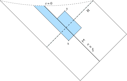
Figure 3.2:

The metric describing this spacetime is given by

$$ds^{2}=-\frac{16M^{3}}{r}e^{-r/{2M}}dudv$$ (3.8)

where we use Kruskal coordinate and $(u,v)$, $r$ is defined implicitly via the following equation

$$uv=(1-\frac{r}{2M})e^{r/{2M}}$$ (3.9)

Since we are dealing with macroscopic black hole, $2M\gg 1$ in causal set units, which is expected to be around Planck scale.

Now let $\Sigma$ be a null hypersurface with equation $v=v_{0}$, and $(x,y)$ be a pair of points satisfying the following conditions Fig (3.2).

$$\left\{\begin{array}[]{c}x\in J^{-}(\Sigma)\cap J^{-}(H)\\ y\in J^{+}(\Sigma)\cap J^{+}(H)\\ x\ \ \mbox{max in}\ J^{-}(\Sigma)\\ y\ \ \mbox{min in}\ J^{+}(\Sigma)\cap J^{+}(H)\\ \end{array}\right.$$ (3.10)

Note that here there is no need to impose the link and the causal relation between $x$ and $y$ since condition (3.10) already imply them.

The volume needed to ensure those conditions can easily be calculated and is given by

$$V=r(\frac{v_{x}}{v_{0}})+r_{0y}^{2}+r_{xy}^{2}-r_{yy}^{2}-r_{x0}^{2}$$

Where we used the following notation

$$u_{i}v_{j}=(1-\frac{r_{ij}}{2M})e^{r_{ij}/{2M}}$$ (3.11)

Now using (3.7) the expected number of links can be written as

$$<n>=(16M^{3})^{2}\int_{0}^{v_{0}}dv_{x}\int_{-\infty}^{0}du_{x}\int_{v_{0}}^{\infty}dv_{y}\int_{0}^{1/v_{y}}du_{y}\frac{e^{-r_{xx}/{2M}}}{r_{xx}}\frac{e^{-r_{yy}/{2M}}}{r_{yy}}\ e^{-V}$$ (3.12)

Now , due to the complicated implicit dependence of the volume on $v_{x},u_{x},v_{y}$ and $u_{y}$ it is very hard to get an exact asymptotic formula for this integral but it is not difficult to show that it is finite and is bounded between the two following value.

$$\frac{\pi^{2}}{6}\leq<n>\leq\frac{\pi^{2}}{3}a$$ (3.13)

Where $a\equiv 2M\gg 1$.

Of course this bound it is not useful, however we will see later that the lower bound must be the exact leading order of the integral. Now, since our aim is to justify the restriction to the flat region in four dimension , we can modify the Max and Min condition slightly to make the calculation possible in both Schwarzschild region and flat region.

To do that let us impose the following conditions.

$$\left\{\begin{array}[]{c}x\in J^{-}(\Sigma)\cap J^{-}(H)\\ y\in J^{+}(\Sigma)\cap J^{+}(H)\\ x\ \ \mbox{max in}\ J^{-}(\Sigma)\cap J^{-}(H)\\ y\ \ \mbox{min in}\ J^{+}(H)\\ \end{array}\right.$$ (3.14)

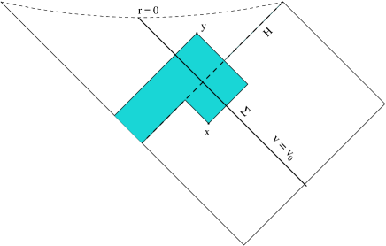
Figure 3.3:

The volume needed to ensure these conditions is evaluated in Appandix A. and is given by, Fig(3.3)

$$V=(2M)^{2}+r_{xy}^{2}-r_{xx}^{2}-r_{yy}^{2}$$ (3.15)

The expected number of links becomes now

$$<n>=(16M^{3})^{2}\int_{0}^{v_{0}}dv_{x}\int_{-\infty}^{0}du_{x}\int_{v_{0}}^{\infty}dv_{y}\int_{0}^{1/v_{y}}du_{y}\frac{e^{-r_{xx}/{2M}}}{r_{xx}}\frac{e^{-r_{yy}/{2M}}}{r_{yy}}e^{-V}$$ (3.16)

Changing the variables

$$(u_{x},v_{x},u_{y},v_{y})\rightarrow(r_{xx},r_{x0},r_{xy},r_{yy})$$

using (3.11) it is easy to evaluate the corresponding Jacobian

$$J=\frac{4}{(16M)^{3}}\frac{r_{xy}}{r_{xy}-2M}\frac{r_{x0}}{r_{x0}-2M}\ r_{xx}\ e^{r_{xx}/{2M}}\ r_{yy}\ e^{r_{yy}/{2M}}$$

where we implemented the notation ( $r_{x0}\equiv r(u_{x}v_{0})$).

Let

$$x=r_{xy},\ y=r_{x0}\ z=r_{xx}$$

Now the boundary of the integral can be easily deduced form (3.11).

We end up with

$$<n>=4(e^{-a^{2}}\int_{0}^{a}e^{r_{yy}^{2}}dr_{yy})I(a)$$ (3.17)

Where $a=2M\gg 1$ for a macroscopic B.H. and

$$I(a)=\int_{a}^{\infty}dx\frac{x}{x-a}e^{-x^{2}}\int_{a}^{x}dy\frac{y}{y-a}\int_{a}^{y}e^{z^{2}}dz$$ (3.18)

In the first place it is interesting to note that the expected number of links does not depend on $v_{0}$ , reflecting the stationarity of spacetime (black hole). In fact any dependence on $v_{0}$ (at least the leading contribution) would kill any hope for this calculation to produce any thing of physical significance, for stationary black holes.

Now, $I(a)$ is shown in Appandix.B to have the following asymptotic expansion,

$$I(a)=\frac{\pi^{2}}{12}a+O(1/a)$$

It is also easy to show that

$$e^{-a^{2}}\int_{0}^{a}e^{r_{yy}^{2}}dr_{yy}=\frac{1}{2a}+O(1/a^{2})$$

Now putting all together we get,

$$<n>=\frac{\pi^{2}}{6}+O(\frac{1}{a})$$ (3.19)

Although the conditions we imposed are not the ones which we will be adopted, this results shows that such counting, were it done in four dimension would turn out to be $v_{0}$-independent and proportional to the area of the horizon namely $(2M)^{2}$.

Before we move to the collapsing null shell let us see where the dominant contributions comes from. To that it is enough to consider only the integral denoted by $I(a)$ .

$$I = \underbrace{\int_{a}^{\infty}\frac{x}{x-a}e^{-x^{2}}dx\int_{a}^{x}dy\int_{a}^{y}e^{z^{2}}dz}_{I_{1}}$$

$$\mbox{}+\underbrace{a\int_{a}^{\infty}\frac{x}{x-a}e^{-x^{2}}dx\int_{a}^{x}\frac{1}{y-a}\int_{a}^{y}e^{z^{2}}dz}_{I_{2}}$$

Let us first concentrate on $I_{1}$.

It is easy to see that $I_{1}$ can be written as

$$I_{1} = \int_{a}^{\infty}\frac{x}{x-a}e^{-x^{2}}dx\int_{a}^{x}dze^{z^{2}}\int_{z}^{x}dy=\int_{a}^{\infty}\frac{x}{x-a}e^{-x^{2}}dx\int_{a}^{x}dze^{z^{2}}(x-z)$$

$$\mbox{}=\int_{a}^{\infty}\frac{x}{x-a}e^{-x^{2}}dx\left[\frac{x}{2z}e^{z^{2}}-\frac{1}{2}e^{z^{2}}\right]_{z=a}^{z=a}+\frac{1}{a}(\mbox{the first term})$$

$$\mbox{}=-\frac{1}{2a}e^{a^{2}}\int_{a}^{\infty}xe^{-x^{2}}+\frac{1}{a}(\mbox{the first term})$$

$$\mbox{}=-\frac{1}{4a}+O(1/a^{2})$$

So we that the term $a$ in the expansion of $I$ must have come from $I_{2}$.

Now

$$I_{2}=a\int_{a}^{\infty}\frac{x}{x-a}e^{-x^{2}}dx\int_{a}^{x}\frac{1}{y-a}\int_{a}^{y}e^{z^{2}}dz$$

The region $y\gg a$ cannot give $a$, because in this region $I_{1}$ is bigger in absolute value than $I_{2}$ as can be easily seen. So the dominant came from $y\rightarrow 0$ and hence from $u_{x}$ near zero, in fact as can be easily seen the term $\frac{1}{y-a}$ diverges at $y=0$ and this what makes it different from $I_{1}$. Although this argument doesn’t say any thing about the pints $y$, the points $y$ which dominate the contribute are the ones sitting near the horizon (null related to the $x$’s ), since other points are exponentially suppressed due to the link and max conditions we are imposing on them. This result shows clearly that this type of counting is controlled by the near horizon geometry; for instance pairs of points $(x,y)$ sitting arbitrarily near to the hypersurface, with $y$ arbitrarily near the horizon, leading to arbitrarily small volume, do not give any significant contribution if $x$ is far from the horizon namely with coordinate $|u_{x}|\gg 1$ ($y\gg a$).

3.3.2 2-dimensional collapsing null matter

We now consider a spherically collapsing null shell of matter with stress energy tensor given by

$$T_{vv}=\frac{M\delta(v-b)}{4\pi r^{2}}$$ (3.20)

the other components are identically zero. Penrose diagram for the spacetime (after dimensional reduction $S^{2}\rightarrow$ point) is shown in Fig(3.4).

Figure 3.4:

Let us chose a null hypersurface $\Sigma$ parameterized by $v=a<b$, Fig(3.5). Here $a$ is of course different from $a$ in the Schwarzschild case.

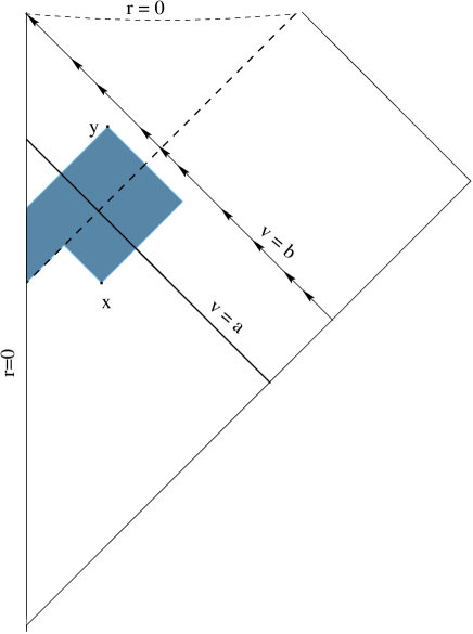
Figure 3.5:

We will assume that $b\gg a\gg 1$ ,the assumption that $b\gg a$ is natural if we want to restrict the counting to the flat region only. The second assumption we take it for the time being as technical, however it will be justified when we deal with the four dimensional case.

Imposing the same Min and Max conditions we imposed in the Schwarzschild case we get for $<n>$ the following expression

$$<n>=\int_{a}^{b}dv_{y}\int_{0}^{v_{y}}du_{y}\int_{\infty}^{0}du_{x}\int_{0}^{a}dv_{x}e^{-V}$$ (3.21)

where

$$V=u_{y}v_{y}-u_{x}(v_{y}-v_{x})-u_{y}^{2}/2$$

It is easy to perform the integration over $v_{x}$ and $u_{x}$, and we end up with

$$<n>=\int_{a}^{b}dv_{y}\int_{0}^{v_{y}}du_{y}\ e^{-u_{y}v_{y}+u_{y}^{2}/2}\ ln\left(\frac{v_{y}}{v_{y}-a}\right)$$

Changing the variables from, $(u_{y},v_{y})$ to $(x=v_{y},y=v_{y}-u_{y})$ we get

$$<n>=\int_{a}^{b}dx\ ln\left(\frac{x}{x-a}\right)e^{-x^{2}/2}\int_{0}^{x}dy\ e^{y^{2}/2}$$

Since $a\leq x\leq b$, and assuming that $a\gg 1$ , it is easy show that

$$e^{-x^{2}/2}\int_{0}^{x}e^{y^{2}/2}dy=\frac{1}{x}+O(\frac{1}{x^{2}})$$

It follows that

$$<n>=\int_{a}^{b}\frac{1}{x}\ ln\left(\frac{x}{x-a}\right)dx+\mbox{higher orders}$$

By higher orders here, we mean terms which are $\leq\frac{1}{a}$ the first term. Now it is also easy to show that

$$\int_{a}^{b}\frac{1}{x}ln\left(\frac{x}{x-a}\right)=\frac{\pi^{2}}{6}-\l(a/b)$$

where

$$l(a/b)=\sum_{k=1}^{\infty}(a/b)^{k}/k^{2}$$

This series is of course convergent and is vanishing in the limit $b\rightarrow\infty$. The presence of the negative contribution $l(a/b)$ is expected, since when $\Sigma$ in near the Schwarzschild region (near the collapse), one should not neglect the links coming from the Schwarzschild which would give a significant contribution .

Now, this result if of interest, by assuming that the collapse is pushed away, or even to future infinity , one can restrict oneself to the flat region and the result would turn out to be the same as the Schwarzschild case, vice-versa , in the collapsing null matter, we can restrict the calculation only in the Schwarzschild region given that the Hypersurface chosen intersects the horizon away from the collapse (in its future). This agreement means that if the calculation were done in four dimension the result will be proportional to the area of the horizon , and the proportionality constant will be the same, in the Schwarzschild case and the flat case, so to establish the area law for the Schwarzschild case it is enough to do calculation in the flat region in the for the collapsing null shell pushing the collapse to future infinity.

Before I move to the 2-d spacelike hypersurface, let me note the following, By imposing the Max and Min which will be adopted for the 4-dimensional, the expected number of links using only the flat region turned out to be (after performing two integral),

$$<n>=\int_{0}^{\infty}ln(\frac{a+y}{y})e^{-(y+a)^{2}/2}dy\int_{y}^{a+y}e^{x^{2}/2}dx$$

and it can easily be shown that:

$$<n>=\frac{\pi^{2}}{6}+O(1/a)$$

This result have two implications. It implies that the lower bound in (3.13) is exactly the leading order of the integral. The other possible implication, is that this type of counting could be insensible to some conditions involving the region inside the black hole. This should not be surprising, since some conditions inside the black could be expected to be irrelevant as far as the conditions have the same behavior near the horizon [44].

3.3.3 Space-like case

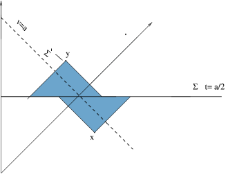
Figure 3.6:

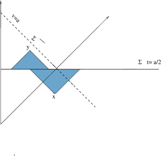
Figure 3.7:

This section we show that doing the calculation in 2-d reduction of 4-d flat using spacelike hypersurface and imposing our Max and Min condition which we will adopt is 4-d the expected number of links is constant, we also show how apparent divergences are cured by the Max and Min and link.

Pushing the collapse to infinity the space time produced is just half of the of the Minkowski spacetime. Consider a space like hypersurface $\Sigma$ with equation $t=a/2$ and consider a pair of points $(x,y)$ satisfying the following conditions.

$$\left\{\begin{array}[]{c}x\in J^{-}(\Sigma)\cap J^{-}(H)\\ y\in J^{+}(\Sigma)\cap J^{+}(H)\\ x\ \ \mbox{max in}\ J^{-}(\Sigma)\\ y\ \ \mbox{min in}\ J^{+}(\Sigma)\cap J^{+}(H)\\ \end{array}\right.$$ (3.22)

Using null coordinate $(u,v)$ we have.

$$\left\{\begin{array}[]{c}v_{x}\leq v_{y}\\ u_{x}+v_{x}\leq a,\ \ u_{x}\leq 0\\ u_{y}+v_{y}\geq a,\ \ v_{y}\geq u_{y}\\ \end{array}\right.$$ (3.23)

In the time like case one has to distinguish different cases for each we have a different volume corresponding to the Max and Min conditions and link.

Let us first introduce a null hypersurface $\Sigma^{\prime}$ with $v=a$ . Now as can be seen Fig(3.6) is qualitatively the same as the contribution we have already evaluated for the null case, so it will just give a constant. Fig(3.7) will not give any significant contribution, because of the Max and Min condition. Now the only possible divergence or some thing different from a constant can only come from contribution of Fig(3.8) and Fig(3.9), and it easy to see that both contributions have the same possible source of apparent divergence, so we will evaluate here just one of them, the other can be shown to be a constant

Now since the apparent divergence due to the pairs with $u_{y}\rightarrow 0$ and $t_{x}=a/2$, we will count just contributions coming from $u_{y}\leq a$ (the other contribution $u_{y}\geq a$ will of course be exponentially suppressed with respect to the one coming form $u_{y}\leq a$.

Now it is easy to read from Fig(3.8) the rang of $u_{x},v_{x},u_{y},v_{y}$.

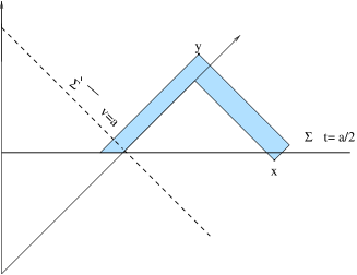
Figure 3.8:

Figure 3.9:

$$\left\{\begin{array}[]{c}a\leq v_{x}\leq v_{y}\\ u_{x}+v_{x}\leq a,\ \ u_{x}\leq 0\\ u_{y}+v_{y}\geq a,\ \ a\leq v_{y}\geq u_{y}\leq a\\ v_{y}+u_{x}\geq a\end{array}\right.$$ (3.24)

The volume needed which will use is the sum of $V_{1}$ and $V_{2}$.

$$V=v_{y}(u_{y}-u_{x})+u_{x}v_{x}-u_{y}a+u_{y}^{2}/2$$ (3.25)

the expected number of links

$$<n>_{a}=\int_{0}^{a}du_{y}\int_{-\infty}^{0}du_{x}\int_{a}^{a-u_{x}}dv_{x}\int_{a-u_{x}}^{\infty}dv_{y}e^{-V}$$ (3.26)

It is easy to perform the integration over $v_{x}$ and $v_{y}$ and we get

$$<n>_{a}=\int_{0}^{a}dy\int_{0}^{\infty}dx\frac{1}{x(y+x)}e^{-xy-y^{2}/2}(1-e^{-x^{2}})=I(a)$$ (3.27)

Where we made a simple change of variables $u_{x}=-x$ and $u_{y}=y$.

To show that $<n>_{a}$ has the following form

$$<n>_{a}=(1)+O(1/a)$$

It is enough to show that $I(\infty)$ is finite.

The only source of divergence of this integral could be from $x\rightarrow\infty$ and $y\rightarrow 0$, so let us study this region.

We first change the variable from $x,y$ to $x,z-x+y$, $I$ becomes

$$I=\int_{0}^{\infty}dx\int_{x}^{\infty}dz\frac{1}{x(z)}e^{-z^{2}/2+x^{2}/2}(1-e^{-x^{2}})$$ (3.28)

Let us split the $I$ into two contributions.

$$(\int_{0}^{\lambda}+\int_{\lambda}^{\infty})dx\frac{e^{x^{2}/2}-e^{-x^{2}/2}}{x}\int_{x}^{\infty}\frac{e^{-z^{2}/2}}{z}$$

Where $\lambda>1$. To prove the convergence of this integral it is enough to prove the convergence of the following integral

$$I_{\lambda}=\int_{\lambda}^{\infty}\frac{e^{x^{2}/2}}{x}\int_{x}^{\infty}\frac{e^{-z^{2}/2}}{z}dz$$

It is easy to see that

$$I_{\lambda}\leq\int_{\lambda}^{\infty}\frac{e^{x^{2}/2}}{x^{2}}dx\int_{x}^{\infty}e^{-z^{2}/2}dz$$

We have also

$$\int_{x}^{\infty}e^{-z^{2}/2}dz=\sqrt{\frac{\pi}{2}}(1-\Phi(\frac{x}{\sqrt{2}}))$$

$$\Rightarrow I_{\lambda}\leq\sqrt{\frac{\pi}{2}}\int_{\lambda}^{\infty}\frac{e^{x^{2}/2}}{x^{2}}(1-\Phi(\frac{x}{\sqrt{2}}))dx\leq$$

$$\sqrt{\frac{\pi}{2\lambda}}\frac{1}{\lambda}\int_{\lambda}^{\infty}\frac{e^{x^{2}/2}}{x^{1/2}}(1-\Phi(\frac{x}{\sqrt{2}}))dx\leq$$

But

$$\int_{\lambda}^{\infty}\frac{e^{x^{2}/2}}{x^{1/2}}(1-\Phi(\frac{x}{\sqrt{2}}))dx$$

is finite, since,

$$\int_{0}^{\infty}\frac{e^{x^{2}/2}}{x^{1/2}}(1-\Phi(\frac{x}{\sqrt{2}}))dx=\frac{1}{2^{5/4}}\Gamma(1/4)$$

The conclusion of this calculation is that once the Max and Min conditions are suitably chosen there can be no divergence and in two dimension the expected number of links is just of order 1, which means that in four dimension the result would turn to be proportional to the area of the horizon.

Before we move to the 4-dimensional case let us see why one would expect the expected number of links to be the same for the null and spacelike hypersurface. Since the counting is based on causal relations and is manifestly Lorentz invariant (in flat case), by Lorentz invariance all space like spacelike planes must give the same answer, but ”in the limit of tilting, a spacelike plane becomes null”. This gives a reason to expect that that null Sigma would produce the same result as spacelike Sigma.

3.3.4 4-dimensional case

Now as we have demonstrated in the previous section that in order to establish the area law one can consider the collapsing null-shell of matter case and pushing the collapse to future .

In 4-dimension if we push the collapse to future infinity, we will mainly be dealing with a cone, and counting the number of links between couple of points $(x,y)$, with the following conditions.

$$\left\{\begin{array}[]{c}x\in J^{-}(H),\ x\ \mbox{max in}J^{-}(\Sigma)\\ y\in J^{+}(H)\cap J^{+}(\Sigma),\ y\ \mbox{min in}J^{+}(H)\cap J^{+}(\Sigma)\\ x\in J^{-}(y)\\ \end{array}\right.$$ (3.29)

Let us use the spherical coordinates and let

$$x=(t_{1},r_{1},\theta_{1},\phi_{1}),\ y=(t_{2},r_{2},\theta_{2},\phi_{2})$$

The above conditions can be written in terms of these coordinates as

$$\left\{\begin{array}[]{c}x\in J^{-}(H)\cap J^{-}(\Sigma)\Rightarrow t_{1}\leq T/2,t_{1}\leq r_{1}\\ y\in J^{+}(H)\cap J^{+}(\Sigma)\Rightarrow t_{2}\geq T/2,r_{2}\leq t_{2}\\ x\in J^{-}(y)\Rightarrow(t_{1}-t_{2})^{2}-(\vec{r_{1}}-\vec{r_{2}})^{2}\geq 0.\\ \end{array}\right.$$ (3.30)

In the 4-dimensional case, the form of the volume needed to ensure the Max and Min conditions depends on the relative position of the points out-in , more precisely depend on the how the light cones of $x$ and $y$ intersect respect to the hypersurface. It turns out [see Appendix.A] that one has to distinguish effectively three categories

a) $t_{1}+t_{2}+\Delta r\leq T$

b)$t_{1}+t_{2}-\Delta r\leq T$

c) $t_{1}+t_{2}-\Delta r\leq T\leq t_{1}+t_{2}+\Delta r\leq T$

In Appendix.A we develop a technique for evaluating those volumes, and evaluate two of them.

For the case (a) the volumes turns out to be particularly simple and is given by the sum of two cones indicated in.

$$V_{a}=\frac{\pi}{3}(t_{1}-\frac{a}{2})^{4}+\frac{\pi}{3}(t_{2}-\frac{a}{2})^{4}$$

Let $x=t_{1}-a/2$ and $y=t_{2}-a/2$.

The expected number of links coming from this type of contributions, can be written as

$$<n>_{a}=\int_{\cal{D}}e^{-\frac{\pi}{3}(x^{4}+y^{4})}dV_{x}dV_{y}$$ (3.31)

where

$$\cal{D}:=\left\{\begin{array}[]{c}0\leq\theta_{i}\leq\pi,\ \ \ 0\leq\phi_{i}\leq 2\pi\\ r_{1}\geq x+a/2,\ \ \ r_{2}\leq y+a/2\\ x\leq 0,\ \ \ y\geq 0\\ \Delta r+x+y\leq 0,\ \ \ \Delta r^{2}-(x-y)^{2}\leq 0\\ \end{array}\right.$$ (3.32)

This integral is evaluated in Appendix.B and it is shown that it has the following asymptotic expansion

$$<n>_{a}=\frac{\pi^{3}a^{2}}{16}(c+(1/a))$$ (3.33)

Where $c$ is given by the equation of appendix

$$c=\int_{0}^{\infty}\int_{0}^{x}(x-y)^{4}e^{-\frac{\pi}{3}(x^{4}+y^{4})}\ dy$$ (3.34)

The other contribution namely $b$ and $c$ are much harder to evaluate due to the complicated algebraic form of the volume however they will give some thing similar to the $a$ except for the proportionality constant, this can be seen easily from the two dimensional case where similar contribution give constant, and the only source for the infinity which may come from points null where $x$ is near $\Sigma$ and point $y$ sitting near the horizon is cured by the Max and Min conditions. Now, since the expression of the volumes for the other cases does not at all suggest that similar exact calculation can be done, one may replace these volumes by an effective volumes obtained by expanding the original ones around their zeros (around the horizon and the values for which the pairs are linked) and keeping only the leading order. And to avoid having contibutions from pairs which do not orginaly contribute (coming from regions far from the horizon), one may add other conevnient volume which would suppress these contributions [Work in this direction is in progress].

Now, if we denote by $\gamma_{c}$ the sum of the different coefficient similar to $c$ and we recover the causal set units we can write for $<n>$

$$<n>=\gamma_{c}\frac{A(\Sigma\cap H)}{l_{c}^{2}}\left(1+(\frac{1}{\sqrt{A}})\right)$$ (3.35)

Where $A(\Sigma\cap H)$ is the area of the cross section in which the horizon $H$ intersect the hypersurface.

If we atribute all the B.H entropy or part of it to $<n>$ we conclude that the causal set scale must be of the order of Planck scale.

Let us now come to our assumption about $a$. Equation (3.33) shows that the number links is proportional to the area of the horizon $A$ , up to corrections which goes like $\frac{1}{\sqrt{A}}$, and as we have seen that the dominant contribution comes from the pair of elements sitting near the horizon, so if the area of the horizon is small in causal set units , the pairs contributing to the expected number of links will be few and as any statistical calculation, this counting will be subjected to statistical fluctuations. Those fluctuations go like $1/\sqrt{<n>}$, hence we may conclude that the subleading term $1/\sqrt{A}$ in the expression of $<n>$ is not too meaningful. Those fluctuations should of course be extremely small if $a\gg 1$ or when one deals with macroscopic black hole and this counting becomes very accurate, in the case of Planck black hole such a counting cannot of course carry over, or even to expect that the entropy will be given by B.H formula.

This observation offers other possible interpretation of this counting, the expected number of links could be understood as a measure of the roughness of the horizon due to the discreteness of the causal set. In counting the links, one could be effectively counting ”horizon elements” of the sort.

3.3.5 Concluding Remarks

We have shown that the expected number of links with natural causality conditions may provide a source of the black hole entropy, and the causal set scale must be of the order of Planck scale beyond which one would expect the continuum description of spacetime to fail and one has only to deal with causal set . Other interesting conclusion, is that these counting is controlled by the near horizon geometry this seems to be in agreement with general idea that the entropy is coming from near horizon states (as Carlip’s [43] calculation and String calculation [40]), and has the advantage that it in principle can be applied in many cases, for instance this counting suggests an entropy for 2+1 black hole also, proportional to the circumference of the horizon.

The interpretation of the black hole entropy as entanglement in-outside the horizon between causal set elements which we started with could be switched to other possible interpretation, namely that by this counting one is measuring the roughness of the horizon due to the discreteness of the causal set.

It should be noted here that this type of counting is not fundamental by itself, or statistical derivation of the B.H entropy, more fundamental derivation and interpretation can only emerge from a better understanding of the causal set dynamics, as for instance the question of the entropy increasing cannot be addressed here, however, if this type of counting turns out to count the number of ”entangled states” defined by tracing out some a well defined quantum states inside the horizon, than the validity of GSL could follow from the proof of reference [42]. What one is merely doing here could be, as we mentioned earlier, similar to counting the number of molecules in a box of gas, which would turn up to a logarithmic factor the entropy of the gas. This result is by itself of interest, since in this way the black hole has revealed for us the discreteness ”atomicity” nature of spacetime, just as the quest for the statistical mechanics of a box of gas tought us something important about the nature of ordinary matter on atomic scales, revealing the existence of atoms and their size.

Appendix 1

Appendix A Evaluation of some volumes

A.1 2- dimensional Schwarzshild spacetime

In this section we evaluate the volume needed to insure the Max and Min and link conditions defined by eqt(3.14) .

$$V=16M^{3}\int_{u_{x}}^{u_{y}}\int_{v_{x}}^{v_{y}}\frac{e^{-r/{2M}}}{r}dudv+16M^{3}\int_{0}^{u_{y}}\int_{0}^{v_{x}}\frac{e^{-r/{2M}}}{r}dudv$$ (A.1)

where $u$ and $v$ are defined implicitly via the following equation

$$uv=(1-r/{2M})e^{r/(2M)}$$ (A.2)

We first evaluate the first part,

$$V_{1}\equiv 16M^{3}\int_{u_{x}}^{u_{y}}\int_{v_{x}}^{v_{y}}\frac{e^{-r/{2M}}}{r}dudv$$

Let us change the variables,

$$(u,v)\rightarrow(u,r(uv)),\Rightarrow dv=-\frac{r}{(2M)^{2}u}e^{r/2M}dr$$

$$\Rightarrow V_{1}=-4M\int_{u_{x}}^{u_{y}}\int_{r(uv_{x})}^{r(uv_{y})}\frac{du}{u}dr=-4M\int_{u_{x}}^{u_{y}}(\frac{r(uv_{y})}{u}-\frac{r(uv_{x})}{u})du$$

We will evaluate the first term .

Let

$$I_{1}\equiv 8M\int_{u_{x}}^{u_{y}}\frac{r(uv_{y})}{u}du$$

$$I_{1}\equiv 8M\int_{u_{x}}^{u_{y}}\frac{r(uv_{x})}{u}du$$

Moving to a new variable,

$$u\rightarrow r(uv_{y})\equiv r_{y},\Rightarrow du=-\frac{r_{y}}{(2M)^{2}}e^{r_{y}/{2M}}dr_{y}$$

$$\Rightarrow I_{1}=\frac{1}{M}\int_{r_{xy}}^{r_{yy}}\frac{r_{y}^{2}}{1-r_{y}/{2M}}dr_{y}=r_{yy}^{2}-r_{xy}^{2}+ln(u_{y}/u_{x})$$

Where we have used eqt(2).

Now, $I_{2}$ can be evaluated in similar fashion, and we get for it ,

$$I_{2}=\frac{1}{M}\int_{r_{xx}}^{r_{yx}}\frac{r_{x}^{2}}{1-r_{x}/{2M}}dr_{y}=r_{yx}^{2}-r_{xx}^{2}+ln(u_{y}/u_{x})$$

$$\Rightarrow V_{1}=r_{yx}^{2}-r_{xx}^{2}+r_{xy}^{2}-r_{yy}^{2}$$

To get the second part of the volume $V$ we just substitute $v_{y}$ and $u_{x}$ by $0$ and use the fact that $r(0)=2M$ .

$$V_{2}=(2M)^{2}-r_{yx}^{2}$$

$$\Rightarrow V=V_{1}+V_{2}=(2M)^{2}+r_{xy}^{2}-r_{xx}^{2}-r_{yy}^{2}$$

A.2 4-dimensional Flat Spacetime

This section we develope a technique for calculating volume needed to ensure maximality and minimality conditions in flat space time.

We will first need the volume of the intersection of two balls (3-d solid sphere), so we start deriving it.

Let $S_{1}$ and $S_{2}$ be two balls with radius $R_{1}$ , $R_{2}$, and centers $\vec{r_{1}}$ , $\vec{r_{2}}$ respectively, and let $S_{1}\cap S_{2}$ denote their intersection. Fig(A.1).

Figure A.1:

First, it is always possible to chose the coordinate system (3-d) such that the equations of the balls take the form.

$$(x-a)^{2}+y^{2}+z^{2}\leq R_{1}^{2}$$

$$x^{2}+y^{2}+z^{2}\leq R_{2}^{2}$$

Now let $x=X_{21}$ denote the equation of the plane that divide the intersection of the two balls to $S_{1}$’s and $S_{2}$’s contribution. Then it is easy to show that

$$X_{21}=\frac{R_{2}^{2}-R_{1}^{2}+a^{2}}{2a}$$ (A.3)

Thus the volume of the intersection can be written as

$$V(S_{1}\cap S_{2})=\pi\int_{a-R_{1}}^{X_{21}}(R_{1}^{2}-(x-a)^{2})dx+\pi\int_{X_{21}}^{R_{2}}(R_{2}^{2}-x^{2})dx$$ (A.4)

It is easy to evaluate the integrals, and the final result is

$$V(S_{1}\cap S_{2})=\pi\left(\frac{2R_{1}^{3}}{3}+\frac{2R_{2}^{3}}{3}-R_{2}^{2}X_{21}-R_{1}^{2}(a-X_{21})+(a-X_{21})^{3}/3+X_{21}^{3}/3\right).$$

Written in invariant form

$$V(S_{1}\cap S_{2})=\pi\left(\frac{2R_{1}^{3}}{3}+\frac{2R_{2}^{3}}{3}-R_{1}^{2}X_{12}-R_{2}^{2}(X_{21})+(X_{12})^{3}/3+X_{21}^{3}/3\right).$$ (A.5)

Where we have used the following notation.

$$X_{21}=\frac{R_{2}^{2}-R_{1}^{2}+{\Delta r}^{2}}{2\Delta r},\ \ \ X_{12}=\frac{R_{1}^{2}-R_{2}^{2}+{\Delta r}^{2}}{2\Delta r}$$

$${\Delta r}^{2}\equiv(\vec{r_{1}}-\vec{r_{2}})^{2}.$$

A.2.1 Volume of the Union of Two Alexandroff Neighborhoods

Other volume which we will need is the the volume of the union of two Alexandroff neighborhoods.

Consider three points in 4-dimensional Minkowskin space, $p_{0}$ , $p_{1}$, $p_{2}$, such that,

$$p_{2}\in J^{+}(p_{1}),\ \ \ p_{2}\in J^{+}(p_{0}),\ \ p_{1}\not\in J^{\mp}(p_{0})$$

The aim is to calculate the the following volume, Fig(A.2).

$$V(J^{+}(p_{0})\cap J^{-}(p_{2})\cup\cap J^{-}(p_{2})\cap J^{+}(p_{1}))$$ (A.6)

Figure A.2:

To do this , we use the freedom, boosts, rotations, translations, and reduce Fig (A.2) to Fig(A.3), namely we choose a coordinate system such that the coordinates of of the points, $p_{0}$, $p_{1}$,and $p_{2}$ are given by

$$p_{1}=(\tau_{1},a,0,0),\ \ \ p_{2}=(\tau_{2},0,0,0),,p_{0}\equiv 0=(0,0,0,0)$$

The equations of the solid light cones are given by

$$(x-a)^{2}+y^{2}+z^{2}\leq(t-\tau_{1})^{2},\ \ \ x^{2}+y^{2}+x^{3}\leq(\tau_{2}-t)^{2},$$

$$x^{2}+y^{2}+x^{3}\leq t^{2}$$

Figure A.3:

In order to evaluate this volume it is necessary to find the times in which the cones intersect. Those times can be easily deduced from the light cone equations.

$$t_{12}=\frac{\tau_{1}+\tau_{2}+a}{2},\ \ \ t_{21}=\frac{\tau_{1}+\tau_{2}-a}{2},$$

$$t_{01}=\frac{\tau_{1}+a}{2},\ \ \ t_{02}=\frac{\tau_{2}}{2}.$$

Fig (A.3) illustrate the evolution of the slicing in time of the volume.

Now using fig(A.4), it is not hard to establish that

$$V(A_{02}\cup A_{12}) = V_{A}(0,2)+\int_{\tau_{1}}^{t_{01}}V(S_{1})+\int_{t_{01}}^{t_{21}}V(\overline{S_{0}\cap S_{1}})+\int_{t_{21}}^{\tau_{2}/2}\overline{S_{0}\cap S_{2}\cap S_{1}}$$

$$= V_{A}(0,2)+\int_{\tau_{1}}^{t_{21}}V(S_{1})+\int_{t_{21}}^{\tau_{2}/2}V(S_{2}\cap S_{1})-\int_{t_{01}}^{\tau_{2}/2}V(S_{0}\cap S_{1})$$

Figure A.4: The shaded parts are the one needed to be included beside the Alsexondroff neighborhood $A(0,2)$. In this figure we chosen $t_{01}\leq t_{21}$, however the form of the integral at the end does not depend on this assumption.

Where,

$$V(S_{2}\cap S_{1}) = \pi(2/3(t-\tau_{1})^{3}+2/3(\tau_{2}-t)^{3}-(t-\tau_{1})^{2}X_{12}-(\tau_{2}-t)^{2}X_{21}$$ (A.7)

$$+X_{12}^{3}/3+X_{21}^{3}/3)$$

$$V(S_{0}\cap S_{1}) = \pi(2/3t^{3}+2/3(t-\tau_{1})^{3}-t^{2}X_{10}-(t-\tau_{1})^{2}X_{01}$$ (A.8)

$$+X_{10}^{3}/3+X_{01}^{3}/3)$$

Where,

$$X_{21}=\frac{\tau_{2}^{2}-\tau_{1}^{2}-2t(\tau_{2}-\tau_{1})+a^{2}}{2a},\ \ \ X_{12}=\frac{\tau_{1}^{2}-\tau_{2}^{2}-2t(\tau_{1}-\tau_{2})+a^{2}}{2a}$$ (A.9)

$$X_{10}=\frac{a^{2}-\tau_{1}^{2}+2t\tau_{1}}{2a},\ \ \ X_{01}=\frac{\tau_{1}+a^{2}-2t\tau_{1}}{2a}$$ (A.10)

Where we have use eqt(A.3) and eqt(A.5). The above integral can easily be calculated and we give only the final answer,

$$\int_{\tau 1}^{t_{21}}V(S_{1})dt=\frac{1}{48}(a+\tau_{1}-\tau_{2})^{4}$$ (A.11)

$$\int_{t_{21}}^{\tau_{2}/2}V(S_{2}\cap S_{1})dt=\frac{1}{24}(a-\tau_{1})(2\tau_{2}a-3\tau_{1}a-\tau_{1}^{2})(a+\tau_{1}-\tau_{2})^{2}/a$$ (A.12)

$$\int_{t_{10}}^{\tau_{2}/2}V(S_{0}\cap S_{1})dt=\frac{1}{48a}(a^{2}-\tau_{1}a+\tau_{2}a-2\tau_{1}^{2})(\tau_{2}-\tau_{1}-a)^{3}$$ (A.13)

And we get for $V$

$$V=V_{A}(2,0)+\frac{1}{24a}(a+\tau_{2})(a-\tau 1)^{2}(a+\tau_{1}-\tau_{2})^{2}$$ (A.14)

Let us no write the volume in a Lorentzian invariant form using the three independent invariant that can be formed from $\tau_{1}$ , $\tau_{2}$ and $a$. These three can be chosen in many ways, however it turns out that the most convenient one are the following

$$B=\tau_{1}^{2}-a^{2}=t_{1}^{2}-r_{1}^{2}$$ (A.15)

$$C=\tau_{2}^{2}=t_{2}^{2}-r_{2}^{2}$$ (A.16)

$$S=t_{1}t_{2}-r_{1}r_{2}\sin\theta_{1}\sin\theta_{2}\cos(\phi_{1}-\phi_{2})$$ (A.17)

Using the above equations it is easy to deduce that,

$$\tau_{1}=\frac{S}{\sqrt{C}}$$ (A.18)

$$a=B+\frac{S^{2}}{4C}$$ (A.19)

After a lengthy algebraic manipulation, $V$ takes the following form,

$$V = \frac{\pi}{24}[(S-B)^{2}+(S-C)^{2}+C(B-C)$$ (A.20)

$$\mbox{}+\frac{(2S^{2}-CB)(C+B)-2S^{3}}{\sqrt{S^{2}-CB}}]$$

To write $V$ in a simpler form , we introduce the following variables,

$$x_{1}=S-B,\ \ \ x_{2}=S-C$$

and let

$$a\equiv x_{1}+x_{2},\ \ \ b\equiv x_{1}x_{2}$$

Using $a$ , $b$ and $S$ as variable $V$ takes the following form,

$$V=a^{2}-b+(s-a)[S+\sqrt{aS-b}]-\frac{bS}{\sqrt{aS-b}}$$ (A.21)

Let us call this volume $V_{m}$.

Now the conditions $p_{2}\in J^{+}(p_{1})$ can be written in terms of $x_{1}$ ,$x_{2}$ and $S$ as

$$x_{1}+x_{2}\leq 0$$ (A.22)

On the other hand we have

$$t_{1}^{2}-r_{1}^{2}\leq 0,\ \ \ t_{2}^{2}-r_{2}^{2}\geq 0$$

it follows that

$$x_{2}\leq x_{1}$$ (A.23)

We conclude that $x_{2}\leq 0$.

Now, as a consistency check for the above result, we will evaluate it for three special cases.

a) If point $p_{1}$ coincides with $p_{0}$ ( in the origin) and $p_{2}$ is arbitrary we have,

$$b=0,\ \ \mbox{ and}\ \ a=-C$$

substituting in eqt(A.21) we get

$$V=\frac{\pi}{24}C^{2}=V_{A}(0,2)$$

As it should be.

b)Another a less trivial check, is for the case when, $p_{1}$ and $p_{2}$ are null related in this case the volume should turn out to be also $V(2,0)$. Using the fact that in this case

$$a=0,\ \ \ b=-x_{2}^{2}=-x_{1}^{2}$$

it is easy to show that $V=V(2,0)$.

c) An other nontrivial check is when $p_{2}$ and $p_{0}$ are null related, in this case the volume should turn out to be just the volume of Alexandroff volume between $p_{1}$ and $p_{2}$, which can be easily checked from the above formula by substituting for $x_{2}=S$ .

A.2.2 Max , Min, and Link conditions

In this section we will use the previous results to deduce the volumes that are needed to ensure Max, Min , Link.[Here we will evaluate the volume for two cases ]

Let $\Sigma$ be a space-like hypersurface with equation $t=T/2$ and let $p_{1}$ and $p_{1}$ be two points with coordinates $(t_{1},r_{1},\theta_{1},\phi_{1})$ and $(t_{2},r_{2},\theta_{2},\phi_{2})$, such that,

$$p_{1}\in J^{-}(p_{2})$$ (A.24)

$$p_{1}\in J^{-}(H)\cap J^{-}(\Sigma)$$ (A.25)

$$p_{2}\in J^{+}(H)\cap J^{+}(\Sigma)$$ (A.26)

$$u_{1}=t_{1}-r_{1}\leq 0\mbox{and}\ v_{1}=t_{1}+r_{1}\geq 0$$ (A.27)

Where $H$ stands for the future light cone of the origin (Horizon).

The aim is to calculate the volume defined by

$$V=V(J^{+}(p_{1})\cap J^{-}(p_{2})\cup J^{+}(p_{1})\cap J^{-}(\Sigma)\cup J^{-}(p_{2})\cap J^{+}(H)\cap J^{+}(\Sigma))$$ (A.28)

Corresponding to the condition that,

$$p_{1}\ \mbox{Max in}\ J^{-}{\Sigma},\ p_{2}\ \mbox{Min in}\ J^{+}(H)\cap J^{+}(\Sigma),\ p_{1}\ \mbox{linked to}\ p_{2}$$ (A.29)

To do this we first have to distinguish three cases depending on the intersections of the past light cone of $p_{2}$ and the boundary of the future light cone of $p_{1}$.

1) If the two intersections happen to be in the past of $\Sigma$ Fig(A.5), the volume is simply given by

$$V=V(J^{+}(p_{1})\cap J^{-}(\Sigma))+V(J^{-}(p_{2})\cap J^{+}(\Sigma))$$ (A.30)

The necessary and sufficient condition to ensure that both intersections are in the past of $\Sigma$ can be deduced easily from the light cones equations and can be written as,

$$\frac{t_{1}+t_{2}+\Delta r}{2}\leq T/2$$ (A.31)

Figure A.5:

2) If the both intersections happen to be in the future of $\Sigma$, Fig(A.6). The necessary and sufficient condition is

$$\frac{t_{1}+t_{2}-\Delta r}{2}\geq T/2$$ (A.32)

Here also one has to distinguish three cases;

2-a)-$v_{2}\geq T$ and $v_{1}\leq T$. Fig(A.6) case 2-a

2-b)-$v_{2}\geq T$ and $v_{1}\geq T$.Fig(A.6) case 2-b 2-c)-$v_{2}\leq T$ and $v_{1}\leq T$.Fig(A.6) case 2-c

Figure A.6:

3)If one intersection is in the future of $\Sigma$ and the other in the past, the necessary and sufficient condition for this is.

$$\frac{t_{1}+t_{2}-\Delta r}{2}\leq T\leq\frac{t_{1}+t_{2}+\Delta r}{2}$$ (A.33)

One has to distinguish also three cases

3-a)-$v_{2}\geq T$ and $v_{1}\leq T$. Fig(A.7) case 3-a

3-b)-$v_{2}\geq T$ and $v_{1}\geq T$.Fig(A.7) case 3-b

3-c)-$v_{2}\leq T$ and $v_{1}\leq T$.Fig(A.7) case 3-c

Figure A.7:

A.2.3 Case 2-a

In this section we will use the results of the previous section to deduce the volume for the case 2-a. To the exception of case 3-a, the other cases may be deduced in similar fashion. For the case 3-a, the procedure developed here fails and one may need to calculated some intersection of three spheres explicitly.

To calculate the volume in case 2-a we choose a coordinate system such that $p_{1}$ and $p_{2}$ lay in the $z$-plane and having the same coordinate $x$

So we have following Cartesian coordinate for $p_{1}$ and $p_{2}$

$$p_{1}=(\tau_{1},a,b,0)\\ \ p_{2}=(\tau_{2},a,c,0)$$

Since we are interested only on the cases which would give a non-suppressed contribution, we will assume that $t_{02}\leq T/2$.

Using the above coordinate the problem is practically reduced to 2+1 problem , and the fig (A.8) show the evolution of the section $z=0$ with time, from which the real 3+1 evolution can be easily deduced. And important parameter of the evolution is the time in which the three $z=0$ section of the three cones intersect at the same point fig(A.8). This is happened in general in two different times, $t_{-}$ and $t_{+}$, these two times can be calculated given the equations of the three light cones, their explicit form is a little complicated and involve a very long calculation to deduce, even though I will give their explicit form here, we will not need them explicitly for calculating the volume $V_{2.a}$.

$$t_{\mp}=\frac{B\mp\sqrt{\Delta}}{4A}$$ (A.34)

Where

$$\Delta=4[r_{1}^{2}r_{2}^{2}-(\vec{r_{1}}\vec{r_{2}})^{2}][(l_{1}\vec{r_{2}}-l_{2}\vec{r_{1}})^{2}-(\tau_{1}l_{2}-\tau_{2}l_{1})^{2}]$$ (A.35)

$$B=2(\tau_{1}\vec{r_{1}}-\tau_{2}\vec{r_{1}})(l_{1}\vec{r_{2}}-l_{2}\vec{r_{1}})$$ (A.36)

$$A=(\tau_{1}\vec{r_{1}}-\tau_{2}\vec{r_{1}})^{2}+(\vec{r_{1}}\vec{r_{2}})^{2}-r_{1}^{2}r_{2}^{2}$$ (A.37)

Figure A.8: This diagramm illustrates the time evolution of section $z=0$ ,for the case 2-a

Using fig(A.8), the volume $V_{2}$ can be written as

$$V_{b} = \int_{\tau_{1}}^{T/2}V(S_{1})+\int_{T/2}^{t_{-}}V(S_{2}\cap S_{0})+\int_{T/2}^{t_{-}}V(\overline{S_{1}\cap S_{0}})$$ (A.38)

$$\mbox{}+\int_{t_{-}}^{t_{+}}V(S_{2}\cap S_{0})+\int_{t_{-}}^{t_{+}}V(\overline{S_{1}\cap S_{0}\cap S_{2}})+\int_{t_{+}}^{\tau_{2}}V(S_{1}\cap S_{2})dt$$

On the other hand, if we use this coordinate system ,$V_{m}$ calculated in the previous section, can be written as

$$V_{m} = \int_{0}^{t_{02}}V(S_{0})+\int_{t_{02}}^{t_{-}}V(S_{2}\cap S_{0})+\int_{\tau_{1}}^{t_{01}}V(S_{1})+\int_{t_{01}}^{t_{-}}V(\overline{S_{1}\cap S_{0}})$$ (A.39)

$$\mbox{}+\int_{t_{-}}^{t_{+}}V(S_{2}\cap S_{0})+\int_{t_{-}}^{t_{+}}V(\overline{S_{1}\cap S_{0}\cap S_{2}})+\int_{t_{+}}^{\tau_{2}}V(S_{1}\cap S_{2})dt$$

Combining eqt(A.38) and eqt(A.39) we deduce that

$$V_{b}=V_{m}+\int_{T/2}^{t_{02}}V(S_{2}\cap S_{0})-\int_{T/2}^{t_{01}}V(S_{1}\cap S_{0})-\int_{0}^{t_{02}}V(S_{0})$$ (A.40)

Where

$$t_{01}=\frac{t_{1}+r_{1}}{2}\ \ \ t_{02}=\frac{t_{2}-r_{2}}{2}$$

Using eqt(A.5), the integrals appearing in eqt(A.40) can easily be evaluated and we quote only the final answer,

$$\int_{T/2}^{t_{01}}V(S_{1}\cap S_{0})dt=\pi\frac{(t_{1}+r_{1}-T)^{3}(Tr_{1}+r_{1}^{2}-2t_{1}^{2}-t_{1}r_{1})}{48r_{1}}$$ (A.41)

$$\int_{T/2}^{t_{02}}V(S_{2}\cap S_{0})dt=\pi\frac{(t_{2}-r_{2})^{2}(T-t_{2}+r_{2})((T-t_{2})^{2}-r_{2}(t_{2}+T))}{24r_{2}}$$ (A.42)

$$\int_{0}^{t_{02}}V(S_{0})=\pi\frac{(t_{2}-r_{2})^{4}}{48}$$ (A.43)

Appendix B Evaluation of some integrals

B.1 Leading order of the Shawrzshild contribution

We evaluate the leading order of the following integral, which appeared chapter 3.

$$I(a)=\int_{0}^{\infty}dx\frac{x}{a-x}\int_{a}^{x}dy\frac{y}{y-a}\int_{a}^{y}e^{z^{2}}dz$$ (B.1)

let

$$I_{1}(y)=\int_{a}^{y}e^{z^{2}}dz$$

$$I_{1}=\sum_{n=0}^{\infty}\frac{y^{2n+1}-a^{2n+1}}{(2n+1)n!}$$

myltiplying $I_{1}$ by $\frac{y}{y-a}$ we get:

$$\frac{y}{y-a}I_{1}\equiv I_{2}(y)=\frac{y}{0!}+\frac{y^{3}+ay^{2}+a^{2}y}{3\times 1!}+\frac{y^{5}+ay^{4}+a^{2}y^{3}+a^{3}y^{2}+a^{4}y}{5\times 2!}+\cdots$$

Now let

$$I_{3}(x)\equiv\frac{1}{x-a}\int_{a}^{x}I_{2}(y)$$

It is easy to show that

$$I_{3}(x) = \frac{a}{1\times 0!}(\frac{(x/a)+1}{2})$$

$$\mbox{}\frac{a^{3}}{3\times 1!}(\frac{(x/a)^{3}+(x/a)^{2}+(x/a)+1}{4}$$

$$\mbox{}+\frac{(x/a)^{2}+(x/a)+1}{3}+\frac{(x/a)+1}{2})$$

$$\mbox{}+\frac{a^{5}}{5\times 2!}(\frac{(x/a)^{5}+(x/a)^{4}+\cdots+1}{6}$$

$$\mbox{}+\frac{(x/a)^{4}+(x/a)^{3}+\cdots+1}{5}+\cdots+\frac{(x/a)+1}{2})$$

$$\mbox{}+\cdots$$

Now the full integral $I(a)$ can be written as

$$I(a) = \frac{a}{1\times 0!}(\frac{J_{2}+J_{1}}{2})$$

$$\mbox{}+\frac{a^{3}}{3\times 1!}(\frac{J_{4}+J_{3}+J_{2}+J_{1}}{4}+\frac{J_{3}+J_{2}+J_{1}}{3}+\frac{J_{2}+J_{1}}{2})$$

$$\mbox{}+\frac{a^{5}}{5\times 2!}(\frac{J_{6}+J_{5}+\cdots+J_{1}}{6}+\frac{J_{5}+\cdots+J_{1}}{5}+\cdots+\frac{J_{2}+J_{1}}{2})$$

where

$$J_{n}\equiv\frac{1}{a^{n-1}}\int_{a}^{\infty}x^{n}e^{-x^{2}}dx.$$

It is easy to show that,

$$J_{n}=\frac{1}{2}e^{-a^{2}}+\frac{n-1}{2a^{2}}J_{n-2},\\ \ J_{1}=\frac{1}{2}e^{-a^{2}}.$$

The $J_{n}$’s with odd $n$ can be evaluted exactly, the ones with $n$ even admit an expansion in $1/a^{2}$. For generic $J_{2n}$ we can write

$$J_{2n} = J_{1}(1+\frac{2n-1}{2a^{2}}+\frac{(2n-1)(2n-3)}{(2a^{2})^{2}}+\cdots$$

$$\mbox{}+\frac{(2n-1)!!}{2a^{2})^{n}}(1-\frac{1}{(2a^{2})^{2}}+\frac{1\times 3}{(2a^{2})^{2}}+\cdots\frac{(-1)^{k}1\times 3\cdots(2k-3)}{(2a^{2})^{k-1}}+\cdots))$$

For genric $J_{2n+1}$

$$J_{2n+1}=J_{1}(1+\frac{2n}{2a^{2}}+\frac{(2n)(2n-2)}{(2a^{2})^{2}}+\cdots+\frac{(2n)!!}{(2a^{2})^{n}})$$

Let us know write $I(a)$ as

$$I(a)=J_{1}(I_{0}+I_{2}+I_{4}+\cdots)$$

Where $I_{2n}$ is obtained by summing terms of order $\frac{1}{a^{2n}}$.

By doing that it can easily be shwon that ,

$$I_{0}=ae^{a^{2}},\ \ \ I_{1}=a(\frac{1}{2^{2}}+\frac{1}{(2a)^{2}})e^{a^{2}}$$

$$I_{2}=a(\frac{1}{3^{2}}+\frac{7}{72a^{2}}-\frac{1}{8a4})e^{a^{2}}$$

$$I_{3}=a(\frac{1}{4^{2}}+\frac{5}{96a^{2}}-\frac{1}{12a^{4}}+\frac{3}{16a^{6}})e^{a^{2}}$$

$$I_{4}=a(\frac{1}{5^{2}}+\frac{13}{400a^{2}}-\frac{143}{2400a^{4}}+\frac{17}{96a^{6}}-\frac{15}{32a^{8}})e^{a^{2}}$$

Now it is easy to read the behavior of the leading term , and the expanison of $I$ may be wriiten as

$$I=\frac{a}{2}(\sum_{n=1}^{\infty}\frac{1}{n^{2}}+\frac{1}{a^{2}}\sum-\frac{1}{a^{4}}\sum+\frac{1}{a^{6}}\sum-\frac{1}{a^{8}}\sum+\cdots)$$

The leading order term is simply given by

$$\frac{a}{2}\sum_{n=1}^{\infty}\frac{1}{n^{2}}=\frac{a\pi^{2}}{12}$$

The other higher order terms are given by other series and as can be seen are raplidly convergent, and the overall series is alternating, howvere it should be noted that this expansion makes sense only for large $a$.

B.2 Evaluation of One 4-dimensional Contribution

This appendix is devoted to the evaluation of the integral which appeared in section chapter3 equation() .

Let

$$I=\int_{\cal{D}}e^{-\frac{\pi}{3}(x^{4}-y^{4})}dV$$ (B.2)

In spherical coordinates $dV$ is given by

$$dV=r_{1}^{2}r_{2}^{2}s_{1}s_{2}d\theta_{1}d\theta_{2}d\phi_{1}d\phi_{2}dr_{1}dr_{2}dxdy,\ \ \ s_{i}\equiv\sin\theta_{i}$$ (B.3)

$$\cal{D}:=\left\{\begin{array}[]{c}0\leq\theta_{i}\leq\pi,\ \ \ 0\leq\phi_{i}\leq 2\pi\\ r_{1}\geq x+a/2,\ \ \ r_{2}\leq y+a/2\\ x\leq 0,\ \ \ y\geq 0\\ \Delta r+x+y\leq 0,\ \ \ \Delta r^{2}-(x-y)^{2}\leq 0\\ \end{array}\right.$$ (B.4)

We make the following change of variables.

$$(x,y,r_{1},r_{2},\theta_{1},\theta_{2},\phi_{1},\phi_{2})\rightarrow(x,y,r_{1},r_{2},\theta_{1},\theta_{2},S,\phi)$$

Where,

$$S=r_{1}r_{2}s_{1}s_{2}cos(\phi_{2}-\phi_{1}),\ \ \ \phi_{1}+\phi_{2}=\phi$$

$$\Rightarrow dV\rightarrow\frac{1}{2}\frac{r_{1}^{2}r_{2}^{2}s_{1}s_{2}}{\sqrt{r_{1}^{2}r_{2}^{2}s_{1}^{2}s_{2}^{2}-S^{2}}}$$

In term of the new variables the domain of integration $\cal{D}$ can be written as

$$\cal{D}:=\left\{\begin{array}[]{c}0\leq\phi\leq 4\pi,\\ r_{1}\geq x+a/2,\ \ \ r_{2}\leq y+a/2\\ -r_{1}r_{2}s_{1}s_{2}\leq S\leq r_{1}r_{2}s_{1}s_{2}\\ 2S\geq r_{1}^{2}+r_{2}^{2}-(x+y)^{2}\\ x+y\leq 0\\ 2S\geq r_{1}^{2}+r_{2}^{2}-(x-y)^{2}\\ \end{array}\right.$$ (B.5)

Note that

$$xy\leq 0\Rightarrow r_{1}^{2}+r_{2}^{2}-(x+y)^{2}\geq r_{1}^{2}+r_{2}^{2}-(x-y)^{2}$$

So we need only to impose the stronger condition on $S$ namely

$$2S\geq r_{1}^{2}+r_{2}^{2}-(x+y)^{2}$$ (B.6)

Let us proceed now.

The integration over $\phi$ gives just $4\pi$ .

To integrate $\theta_{1}$ we note that from the condition

$$-r_{1}r_{2}s_{1}s_{2}\leq S\leq r_{1}r_{2}s_{1}s_{2}$$

we deduce

$$-\sqrt{1-\frac{S^{2}}{(r_{1}r_{2})^{2}s_{2}^{2}}}\leq\cos\theta_{1}\leq\sqrt{1-\frac{S^{2}}{(r_{1}r_{2})^{2}s_{2}^{2}}}$$ (B.7)

$$\Rightarrow\theta_{-}\equiv\arccos(-\sqrt{1-\frac{S^{2}}{(r_{1}r_{2})^{2}}})\leq\theta_{2}\leq\arccos(\sqrt{1-\frac{S^{2}}{(r_{1}r_{2})^{2}}})\equiv\theta_{+}$$ (B.8)

It is easy to show that

$$\int_{\theta_{-}}^{\theta_{+}}\frac{s_{1}}{\sqrt{(r_{1}r_{2}s_{1}s_{2})^{2}-S^{2}}}=\frac{\pi}{r_{1}r_{2}s_{2}}$$ (B.9)

The integration over $\theta_{2}$ becomes trivial and we end up with

$$I=2\pi^{2}r_{1}r_{2}[\pi-2\arccos(\sqrt{1-\frac{S^{2}}{(r_{1}r_{2})^{2}}})]\ e^{-V}\ dSdr_{1}dr_{2}dxdy$$ (B.10)

To integrate over $S$ we have to distinguish many case, depending on the range of the other variables, this can be done by studying the domain of integration $\cal{D}$, which is not hard, once that is done, the domain $\cal{D}$ splits into the following domains.

-A): $S\geq 0$

$${\cal{D}}(A.1):\left\{\begin{array}[]{c}2r_{1}r_{2}\geq 2S\geq r_{1}^{2}+r_{2}^{2}-(x+y)^{2}\geq 0\\ r_{2}-x-y\geq r_{1}\geq r_{2}+x+y\\ y+a/2\geq r_{2}\geq a/2-y\\ -y\geq x\geq-a/2\\ a/2\geq y\geq 0\\ \end{array}\right.$$ (B.11)

$${\cal{D}}(A.2):\left\{\begin{array}[]{c}2r_{1}r_{2}\geq 2S\geq r_{1}^{2}+r_{2}^{2}-(x+y)^{2}\geq 0\\ r_{2}-x-y\geq r_{1}\geq r_{2}+x+y\\ y+a/2\geq r_{2}\geq-x-y\\ x\leq-a/2\\ \end{array}\right.$$ (B.12)

$${\cal{D}}(A.3):\left\{\begin{array}[]{c}2r_{1}r_{2}\geq 2S\geq r_{1}^{2}+r_{2}^{2}-(x+y)^{2}\geq 0\\ r_{2}-x-y\geq r_{1}\geq x+a/2\\ 2x+y+a/2\leq r_{2}\leq a/2-y\\ -x\geq y\geq-3/2x-a/4\\ -a/2\leq x\leq-a/6\\ \end{array}\right.$$ (B.13)

$${\cal{D}}(A.4):\left\{\begin{array}[]{c}2r_{1}r_{2}\geq 2S\geq r_{1}^{2}+r_{2}^{2}-(x+y)^{2}\geq 0\\ r_{2}-x-y\geq r_{1}\geq x+a/2\\ 2x+y+a/2\leq r_{2}\leq a/2-y\\ -x\geq y\geq 0\\ 0\geq x\geq-a/6\\ \end{array}\right.$$ (B.14)

$${\cal{D}}(A.5):\left\{\begin{array}[]{c}2r_{1}r_{2}\geq 2S\geq r_{1}^{2}+r_{2}^{2}-(x+y)^{2}\geq 0\\ r_{2}-x-y\geq r_{1}\geq x+a/2\\ -x-y\leq r_{2}\leq a/2-y\\ -3/2x-a/4\geq y\geq 0\\ -a/6\geq x\geq-a/2\\ \end{array}\right.$$ (B.15)

$${\cal{D}}(A.6):\left\{\begin{array}[]{c}2r_{1}r_{2}\geq 2S\geq 0\geq r_{1}^{2}+r_{2}^{2}-(x+y)^{2}\\ x+a/2\leq 0\leq r_{1}\leq\sqrt{(x+y)^{2}-r_{2}^{2}}\\ 0\leq r_{2}\leq-x-y,y+a/2\\ x\leq-a/2\\ \end{array}\right.$$ (B.16)

$${\cal{D}}(A.7):\left\{\begin{array}[]{c}2r_{1}r_{2}\geq 2S\geq 0\geq r_{1}^{2}+r_{2}^{2}-(x+y)^{2}\\ x+a/2\leq r_{1}\leq\sqrt{(x+y)^{2}-r_{2}^{2}}\\ y\leq a/2,x\leq-a/4\\ \end{array}\right.$$ (B.17)

$${\cal{D}}(A.7):\left\{\begin{array}[]{c}2r_{1}r_{2}\geq 2S\geq 0\geq r_{1}^{2}+r_{2}^{2}-(x+y)^{2}\\ x+a/2\leq r_{1}\leq\sqrt{(x+y)^{2}-r_{2}^{2}}\\ y\geq a/2\end{array}\right.$$ (B.18)

-B): $S\leq 0$.

$${\cal{D}}(B.1):\left\{\begin{array}[]{c}0\geq 2S\geq-2r_{1}r_{2}\geq r_{1}^{2}+r_{2}^{2}-(x+y)^{2}\\ 0\leq x+a/2\leq r_{1}\leq-r_{2}-x-y\\ 0\leq r_{2}\leq-2x-y-a/2\\ 0\leq y\leq-2x-a/2\\ x\leq-a/4\end{array}\right.$$ (B.19)

$${\cal{D}}(B.2):\left\{\begin{array}[]{c}0\geq 2S\geq-2r_{1}r_{2}\geq r_{1}^{2}+r_{2}^{2}-(x+y)^{2}\\ x+a/2\leq 0\leq r_{1}\leq-r_{2}-x-y\\ x\leq-a/2\end{array}\right.$$ (B.20)

$${\cal{D}}(B.3):\left\{\begin{array}[]{c}0\geq 2S\geq r_{1}^{2}+r_{2}^{2}-(x+y)^{2}\geq-2r_{1}r_{2}\\ \sqrt{(x+y)^{2}-r_{2}^{2}}\geq r_{1}\geq-r_{2}-x-y\\ 0\leq r_{2}\leq-x-y\\ x\leq-a/2\\ \end{array}\right.$$ (B.21)

$${\cal{D}}(B.4):\left\{\begin{array}[]{c}0\geq 2S\geq r_{1}^{2}+r_{2}^{2}-(x+y)^{2}\geq-2r_{1}r_{2}\\ \sqrt{(x+y)^{2}-r_{2}^{2}}\geq r_{1}\geq-r_{2}-x-y\\ 0\leq r_{2}\leq y+a/2\\ x\leq-a/4\end{array}\right.$$ (B.22)

$${\cal{D}}(B.5):\left\{\begin{array}[]{c}\sqrt{(x+y)^{2}-r_{2}}\geq r_{1}\geq x+a/2\\ -2x-y-a/2\leq r_{2}\leq y+a/2\\ y\geq a/2\end{array}\right.$$ (B.23)

Now except the domain ${\cal{D}}(A.1)$ and ${\cal{D}}(A.4)$, the others give a exponentially suppressed contributions.This can be seen as follow. If $|x|$ or $y$ $\geq ca$ (for some $c$ of order 1), the volume in the exponential is always bigger than some thing like $a^{4}$ which will always factor out at the end of the calculation and since the large $x$ and $y$ are exponentially suppressed (no null contribution in this case), the final result will be at most some thing like $poly(a)e^{-a^{4}}$, or more precisely $a^{2}e^{-a^{4}}$.

Let us now evaluate the contribution ${\cal{D}}(A.1)$ and ${\cal{D}}(A.4)$

We will use the following notation

$$z=r_{1},\ \ \alpha=r_{2}^{2}-(x+y)^{2}\geq 0,\ \ \ t=r_{2}\geq 0$$ (B.24)

Let

$$I(z)=\int_{\frac{z^{2}+\alpha}{2}}^{r_{1}r_{2}}r_{1}r_{2}(\pi-2\arcsin(\frac{S}{r_{1}r_{2}}))dS$$ (B.25)

This integral is easy to evaluate and the result is,

$$I(z)=zt\left[\frac{\pi}{2}[z^{2}+\alpha]-[z^{2}+\alpha]\arcsin[\frac{z^{2}+\alpha}{2zt}]-\sqrt{4z^{2}t^{2}-(z^{2}+\alpha)^{2}}\right]$$ (B.26)

To integral over $z=r_{1}$, we let

$$I_{1}=\int(\frac{z^{2}+\alpha}{2})zdz$$ (B.27)

$$I_{2}=\int z(z^{2}+\alpha)\arcsin(\frac{z^{2}+\alpha}{2z\beta})dz$$ (B.28)

$$I_{3}=\int z\sqrt{4z^{2}\beta^{2}-(z^{2}+\alpha)^{2}}dz$$ (B.29)

All the above integrals can be evaluated and we only quote the result

$$I_{1}=\frac{z^{2}}{4}(\frac{z^{2}}{2}+\alpha)$$ (B.30)

$$I_{2} = \frac{z^{2}}{2}(\frac{z^{2}}{2}+\alpha)\arcsin(\frac{z^{2}+\alpha}{2zt})$$ (B.31)

$$-\frac{1}{8}[2(3t^{4}-2t^{2}\alpha-\alpha^{2})\arcsin[\frac{1}{2}\frac{z^{2}+2t^{2}-\alpha}{\sqrt{t^{2}(t^{2}-\alpha)}}]$$

$$+\frac{1}{2}(\frac{\alpha}{2}-3t^{2}-\frac{z^{2}}{2})\sqrt{4z^{2}t^{2}-(z^{2}+\alpha)^{2}}]$$

$$I_{3} = t^{2}(\beta^{2}-\alpha)\arcsin[\frac{z^{2}+2t^{2}-\alpha}{t^{2}(t^{2}-\alpha)}]$$ (B.32)

$$+\frac{1}{4}(z^{2}-2t^{2}+\alpha)\sqrt{4z^{2}t^{2}-(z^{2}+\alpha)^{2}}$$

Now

$$\int I(z)dz = I_{1}-I_{2}-I_{3}=\frac{1}{4}z^{2}[\frac{z^{2}}{2}+\alpha][\pi-2\arcsin(\frac{z^{2}+\alpha}{2zt})]$$ (B.33)

$$-\frac{1}{4}[t^{2}-\alpha]^{2}\arcsin\left[\frac{z^{2}-2t^{2}+\alpha}{2\sqrt{t^{2}(t^{2}-\alpha)}}\right]$$

$$+\frac{1}{16}[2t^{2}-3\alpha-5z^{2}]\sqrt{4z^{2}t^{2}-(z^{2}+\alpha)^{2}}$$

We start with the case ${\cal{D}}(A.4)$

We introduce the following notation

$$\alpha_{+}=a/2-y,\ \ \ \alpha_{-}=2x+y+a/2$$ (B.34)

$$\int_{\alpha_{-}}^{\alpha_{+}}I_{z}dz = \frac{1}{8}(\frac{\alpha_{+}-\alpha_{-}}{2})^{4}t(\pi-\arcsin\left[\frac{\alpha_{-}\alpha_{+}-t^{2}}{t(\alpha_{+}-\alpha_{-})}\right])$$ (B.35)

$$+\frac{1}{128}t(\alpha_{-}+\alpha_{+})^{2}[8t^{2}-\alpha_{-}^{2}-\alpha_{+}^{2}+6\alpha_{-}\alpha_{+}](\pi$$

$$-2\arcsin\left[\frac{\alpha_{+}\alpha_{-}+t^{2}}{t(\alpha_{+}+\alpha_{+})}\right])$$

$$-\frac{1}{16}[\frac{1}{2}\alpha_{-}^{2}+\frac{1}{2}\alpha_{+}^{2}+4\alpha_{+}\alpha_{-}+t^{2}]\sqrt{(\alpha_{+}^{2}-t^{2})(t^{2}-\alpha_{-}^{2})}$$

Let

$$f_{0}=\frac{1}{128}t(\alpha_{-}+\alpha_{+})^{2}[8t^{2}-\alpha_{-}^{2}-\alpha_{+}^{2}+6\alpha_{-}\alpha_{+}]$$ (B.36)

$$f_{1}=-\frac{t}{64}(\alpha_{-}+\alpha_{+})^{2}[8t^{2}-\alpha_{+}^{2}-\alpha_{-}^{2}+6\alpha_{-}\alpha_{+}]\arcsin\left[\frac{\alpha_{-}\alpha_{+}+t^{2}}{t(\alpha_{-}+\alpha_{+})}\right]$$ (B.37)

$$f_{2}=-\frac{1}{4}(\frac{\alpha_{+}-\alpha_{-}}{2})^{4}t\arcsin\left[\frac{\alpha_{-}\alpha_{+}-t^{2}}{t(\alpha_{+}-\alpha_{-})}\right]$$ (B.38)

$$f_{3}=-\frac{1}{16}[\frac{1}{2}\alpha_{-}^{2}+\frac{1}{2}\alpha_{+}^{2}+4\alpha_{+}\alpha_{-}+t^{2}]\sqrt{(\alpha_{+}^{2}-t^{2})(t^{2}-\alpha_{-}^{2})}$$ (B.39)

$$f_{4}=\frac{\pi}{8}t(\frac{\alpha_{+}-\alpha_{-}}{2})^{4}$$ (B.40)

We have

$$\int f_{0}=\frac{t^{2}}{256}(\alpha_{-}+\alpha_{+})^{2}[4t^{2}-\alpha_{-}^{2}-\alpha_{+}^{2}+6\alpha_{-}\alpha_{+}]\arcsin\left[\frac{\alpha_{-}\alpha_{+}+t^{2}}{t(\alpha_{-}+\alpha_{+})}\right]\$$ (B.41)

$$\int f_{1}dt = -\frac{t^{2}}{128}(\alpha_{-}+\alpha_{+})^{2}[4t^{2}-\alpha_{-}^{2}-\alpha_{+}^{2}+6\alpha_{-}\alpha_{+}]\arcsin\left[\frac{\alpha_{-}\alpha_{+}+t^{2}}{t(\alpha_{-}+\alpha_{+})}\right]$$ (B.42)

$$+\frac{1}{256}(\alpha_{+}^{2}-\alpha_{-}^{2})^{2}(\alpha_{+}^{2}+\alpha_{-}^{2}+4\alpha_{-}\alpha_{+})\arcsin\left[\frac{2t^{2}-\alpha_{-}^{2}-\alpha_{+}^{2}}{\alpha_{+}^{2}-\alpha_{-}^{2}}\right]$$

$$-\frac{1}{128}(\alpha_{-}+\alpha_{-})^{2}[\alpha_{-}^{2}+\alpha_{-}^{2}+\alpha_{-}\alpha_{+}+t^{2}]\sqrt{(\alpha_{-}^{2}-t^{2})(t^{2}-\alpha_{2}^{2})}$$

$$\int f_{2} = -\frac{1}{8}(\frac{\alpha_{-}-\alpha_{+}}{2})^{2}t^{2}\arcsin\left[\frac{\alpha_{-}\alpha_{+}-t^{2}}{t(\alpha_{+}-\alpha_{-})}\right]$$ (B.43)

$$+\frac{1}{32}(\frac{\alpha_{+}-\alpha_{-}}{2})^{2}(\alpha_{-}+\alpha_{-})^{2}\arcsin\left[\frac{2t^{2}-\alpha_{-}^{2}-\alpha_{+}^{2}}{\alpha_{+}^{2}-\alpha_{-}^{2}}\right]$$

$$-\frac{1}{8}(\frac{\alpha_{+}-\alpha_{-}}{2})^{4}t^{2}\arcsin\left[\frac{\alpha_{-}\alpha_{+}-t^{2}}{t(\alpha_{+}-\alpha_{-})}\right]$$

$$-poly(t)\sqrt{(t^{2}-\alpha_{-}^{2})(\alpha_{+}-t^{2})}$$

$$\int f_{3} = -\frac{1}{64}(\frac{\alpha_{+}^{2}-\alpha_{-}^{2}}{2})^{2}[\alpha_{-}^{2}+\alpha_{+}^{2}+4\alpha_{-}\alpha_{+}]\arcsin\left[\frac{2t^{2}-\alpha_{-}^{2}-\alpha_{+}^{2}}{\alpha_{+}^{2}-\alpha_{-}^{2}}\right]$$ (B.44)

$$+poly(t)\sqrt{(t^{2}-\alpha_{-}^{2})(\alpha_{+}^{2}-t^{2})}$$

$$\int f_{4}=\frac{\pi}{16}(\frac{\alpha_{+}-\alpha_{-}}{2})^{4}t^{2}$$ (B.45)

Evaluating these integrals between $\alpha_{-}$ and $\alpha_{+}$, we get

$$\int_{\alpha_{-}}^{\alpha_{+}}(f_{0}+f_{1})=\frac{\pi}{256}(\alpha_{+}^{2}-\alpha_{-}^{2})^{2}(\alpha_{-}^{2}+\alpha_{+}^{2}+4\alpha_{-}\alpha_{+})$$ (B.46)

$$\int_{\alpha_{-}}^{\alpha_{+}}f_{2}=\frac{\pi}{32}(\frac{\alpha_{+}-\alpha_{-}}{2})^{4}\left((\alpha_{-}+\alpha_{+})^{2}+2(\alpha_{-}^{2}+\alpha_{+}^{2})\right)$$ (B.47)

$$\int_{\alpha_{-}}^{\alpha_{+}}f_{3}=-\frac{\pi}{256}(\alpha_{+}^{2}-\alpha_{-}^{2})^{2}(\alpha_{-}^{2}+\alpha_{+}^{2}+4\alpha_{-}\alpha_{+})$$ (B.48)

$$\int_{\alpha_{-}}^{\alpha_{+}}f_{4}=\frac{\pi}{16}(\frac{\alpha_{+}-\alpha_{-}}{2})^{4}(\alpha_{+}^{2}-\alpha_{-}^{2})$$ (B.49)

Summing up all the contribution we end up

$$I({\cal{D}}(A.4))\equiv I_{1}=\frac{\pi}{32}(\frac{\alpha_{-}-\alpha_{+}}{2})^{4}\left[(\alpha_{-}+\alpha_{+})^{2}+4\alpha_{+}^{2}\right]$$ (B.50)

Thus the contribution of ${\cal{D}}(A.4)$ to the expected number of links is

$$<n>_{4} = \frac{\pi^{3}}{8}\int_{-a/6}^{0}\int_{0}^{-x}(x+y)^{4}[(x+a/2)^{2}+(a/2-y)^{2}]e^{-\frac{\pi}{3}(x^{4}+y^{4})}dxdy$$ (B.51)

$$=\frac{\pi^{3}}{8}\int_{0}^{a/6}\int_{0}^{x}(x-y)^{4}[(x-a/2)^{2}+(a/2-y)^{2}]e^{-\frac{\pi}{3}(x^{4}+y^{4})}dxdy$$

It is not hard to see that this integral will have the following expansion

$$<n>_{4}=\frac{\pi^{3}}{16}a^{2}(c+(1/a))$$ (B.52)

Where

$$c=\int_{0}^{\infty}dx\int_{0}^{x}(x-y)^{4}\ e^{-\frac{\pi}{3}(x^{4}+y^{4})}\ dy$$ (B.53)

For the case ${\cal{D}}(A.1)$ we have

$$I_{z}(t+x+y)-I_{z}(t-x-y)=\frac{\pi}{4}(x+y)^{4}t$$ (B.54)

The contribution of ${\cal{D}}(A.1)$ to $<n>$ is given by

$$<n>_{1} = \frac{\pi}{2}\int_{-a/2}^{0}dx\int_{0}^{-x}(x+y)^{4}\ dy\int_{a/2-y}^{a/2+y}t\ e^{-V(x,y)}dt$$ (B.55)

$$=\frac{\pi^{3}a}{2}\int_{-a/2}^{0}dx\int_{0}^{-x}y(x+y)^{4}\ e^{-\frac{\pi}{3}x^{4}-\frac{\pi}{3}y^{4}}\ dy$$

$$=\frac{\pi^{3}a}{2}\int_{0}^{a/2}dx\int_{0}^{x}y(x-y)^{4}e^{-\frac{\pi}{3}(x^{4}+y^{4})}\ dy$$

Now it is not difficult to see that the result must has the following form

$$<n>_{1}=\frac{\pi^{3}a}{2}(c_{1}+(1/a))$$ (B.56)

where

$$c_{1}=\int_{0}^{\infty}dx\int_{0}^{x}y(x-y)^{4}e^{-\frac{\pi}{3}(x^{4}+y^{4})}\ dy$$ (B.57)

Summing up,

$$<n>=\frac{\pi^{3}}{16}a^{2}(c+(1/a))$$ (B.58)

Bibliography

- [1] R.Sorkin, gr-qc/9706002
- [2] C.J.Isham, gr-qc/9510063
- [3] C. Rovelli, gr-qc/9903045
- [4] J.Polchinski, Int I.Mod.Phys. A14,(1999) 2633-2658.
- [5] G.’t Hooft, ” Recent Developments in Gravitaion”(Proceedings of the 1978 Cargese Summer Institute) edited by M.Levy and S.Deser (Plenum 1979), pp.323-45.
- [6] J.Myrheim, CERN Report No. TH-2538, 1978 (unpublished).
-
[7]
L.Bombelli, J.Lee, D.Meyer, and R.Sorkin, Phys.Rev.Lett. 59, 521-24
(1987);
Phys.Rev.Lett. 60, 656 (1988). - [8] Luca Bombelli, Ph.D thesis, Syracuse, 1987.
- [9] D.Meyer ,Ph.D thesis, MIT, 1988.
- [10] R.D.Sorkin, A Specimen of Theory Construction from Quantum Gravity, in ”The Creation of Ideas in Physics”, ed. Jarrett Leplin, (Kluwer Academic Publishers, Dordrecht, 1995), gr-qc/9511063.
- [11] R.D.Sorkin, ”Spacetime and Causal Sets”, in J.C.D’Olivo, E.Nahmad-Achar, M.Rosenbaum, M.P. Rayan, L.F.Urrutia and F.Zertuche (eds), Relativity and Gravitation:Classical and Quantum, (Proceedings of the SILARG Conference, held Cocoyoc, Mexico, December, 1990), pages 150-173.
- [12] S.Weinberg, Qunatum Field Theory vol2.
- [13] D.P.Rideout and R.D.Sorkin, gr-qc/9904062.
- [14] J.F.Donoghue, T.Torma, Phy.Rev.D 60(1999) 024003, and references therein.
- [15] Djamel.Dou, Roberto Percacci, Class.Quant.Grav.15 (1998)3449-3488.
- [16] M.Reuter, Phy.Rev.D 57(1998) 971-985.
- [17] S.W.Hawking, A.R.King, and P.J.McCarthy, J.Math.Phys.17,174-181 (1976).
- [18] D.Malament, J.Math.Phys.18, 1399-1404 (1977).
- [19] T.D.Lee, in How Far Are We from the Gauge Forces?, edited by A.Zichichi (Plenum, New York, 1985).
- [20] G.Brightwell, Winkler.P, Order 6, 235 (1989).
- [21] William Trotter, S. Felsner and P. C. Fishburn, ”Finite three dimensional partial orders which are not sphere orders”, Discrete Math. 201, 101-132 (1999).
- [22] D.P.Rideout, Causal Set Dynamics, Ph.D thesis 1999, University of Syracuse (in preparation).
- [23] A.R.Daughton, The Recovery of Locality for Causal sets and Related Topics, Ph.D thesis, Syracuse Universty (May 1993).
- [24] Rob.Sgandalo, (in preparation).
- [25] J.D.Bekenstein, Lett.Nuov.Cimento 4 (1972) 737.
- [26] J.D.Bekenstein, phys.Rev.D 7(1973) 2333.
- [27] J.D.Bekenstein, Plenary talk at Seventh Marcel Grossman meeting at Stanford University, gr-qc/9409015.
- [28] S.Hwaking, Nature (physical Science) 248 (1974) 30.
- [29] S.W.Hawking, Commun.Math.Phy 43(1975) 199.
- [30] J.W.Bardeen, B.Carter, S.W.Hawking . (1973) Commun.Math.Phy.31, 161.
- [31] G.Gibbons and S.W.Hawking, Phys.Rev.D 15, 2752 (1977)
- [32] R.Wald, Quantum Field Theory in Curved Spacetime, and Black Hole Thermodynamics.
- [33] R.Wald, Black Holes and Thermodynamics, in Black Holes and Relativistic Stars, edited by R.Wald (University of Chicago Press, 1998).
- [34] R.Sorkin, The Stistical Mechanics of Black Hole Thermodynamics,in Black Holes and Relativistic Stars, edited by R.Wald (University of Chicago Press, 1998).
- [35] R.Sorkin, ”On the Entropy of the Vacuum Outside a Horizon”, in B.Bertotti, F.de Felice, Pascolini, (eds.), Tenth International Conference on General Relativity and Gravitation (held Padova, 4-9 July, 1983), Contributed Papers, Vol.2 pp.734-736 (Roma, Consiglio Nazionale Delle Ricerche, 1983)
- [36] James B.Hartle, Generalized Quantum Theory in Evaporating Black Hole Spacetimes, in Black Holes and Relativistic Stars, edited by R.Wald (University of Chicago Press, 1998).
- [37] L.Bombelli, R.Koul, J.Lee and R.Sorkin, Phys.Rec. D 34 (1986) 373.
- [38] M.Sredincki, Phys.Rev.D 71 (1976) 107.
- [39] C.Callan and F.Wilczek, Phys. Lett. B 333 (1994) 55-61
- [40] L.Susskind and J.Uglum, Phys.Rev. D50 (1994) 2700-2711
- [41] D.Kabat and F.J.Strassler, Phys.Lett. B329 (1994) 46-52
- [42] R.D.Sorkin, Phys.Rev.lett. 56 (1986) 1885.
- [43] S.Carlip, Class.Quant.Grav. 16 (1999) 3327-3348
- [44] Dou.Djamel, R.D.Sorkin, Black Hole Entropy as Links (in preparation)