Machian General Relativity: a possible solution to the Dark Energy problem and an alternative to Big Bang cosmology
Abstract
Observations of an apparent acceleration in the expansion rate of the Universe, derived from measurements of high-redshift supernovae, have been used to support the hypothesis that the Universe is permeated by some form of dark energy. We show that an alternative cosmological model, based on a linearly expanding Universe with Omega=1, can fully account for these observations. This model is also able to resolve the other problems associated with the standard Big Bang model. A scale-invariant form of the field equations of General Relativity is postulated, based on the replacement of the Newtonian gravitational constant by an formulation based explicitly on Mach’s principle. We derive the resulting dynamical equations, and show that their solutions describe a linearly expanding Universe. Potential problems with non-zero divergencies in the modified field equations are shown to be resolved by adopting a radically different definition of time, in which the unit of time is a function of the scale-factor. We observe that the effects of the modified field equations are broadly equivalent to a Newtonian gravitational constant that varies both in time and in space, and show that this is also equivalent to Varying Speed of Light (VSL) theories using a standard definition of time. Some of the implications of this observation are discussed in relation to Black Holes and Planck scale phenomena. We examine the consequences of the definition of time inherent in this model, and find that it requires a reappraisal of the standard formula for the energy of a photon. An experiment is proposed that could be used to verify the validity of this cosmological model, by measuring the noise power spectrum of the Cosmic Microwave Background (CMB). An alternative scenario for the early stages of the evolution of the Universe is suggested, based on an initially cold state. It is shown that this can in principle lead to primordial nucleosynthesis of the light elements. Finally, we examine some of the other potential consequences that would follow from the model, including the possibility of reconciling the paradox of non-locality inherent in Quantum Mechanics, the avoidance of an initial singularity, and the ultimate fate of the Universe.
1 Introduction
1.1 Big Bang problems
Our ideas about the origin and evolution of the Universe have developed markedly since the discovery of the Red Shift by Hubble in 1935. This phenomenon has lead to the conclusion that the galaxies must be receding from each other. This leads to two possibilities; either the galaxies were once close together and ‘exploded’ apart in a ‘Big Bang’, or the Universe is in a steady state, with matter being continually created so as to maintain the matter density of the Universe at a constant value as it expands. The subsequent discovery of the microwave background radiation in 1965 suggests strongly that the Big Bang theory is the correct one. However, the Big Bang theory, whilst very successful in explaining many features of the Universe including the origins and relative abundances of the elements, does not fully account for a number of observations about the large scale structures in the Universe. It also leads to disturbing conclusions about the state of the Universe at times close to the origin of the Big Bang and at times near the end of the life of the Universe.
The standard cosmological problems are well documented in a number of sources, including [19]. A brief summary of the principal issues is given here.
1.1.1 The horizon problem
The standard theory is unable to explain how regions of the Universe that had not been in contact with each other since the Big Bang are observed to emit cosmic background radiation at almost precisely the same temperature as each other. A related problem is the explanation for galaxy formation. Recent results from COBE and other surveys of the cosmic microwave background suggest that there were small fluctuations in the distribution of matter within the Universe at the epoch of radiation decoupling which could account for the range of large scale structures that are observed in the Universe. If the Universe was initially perfectly smooth, by what mechanism did matter start to clump together to form stars, galaxies, and galaxy clusters ?
1.1.2 The flatness problem
The fact that the observed matter density of the Universe is so close to the critical value necessary for the Universe to be closed implies that the ratio of these densities, , must have been very close to one at the time of the Big Bang. This observation is the one of the main reasons for the widely held belief that there is probably additional hidden mass in the Universe such that is in fact equal to one in the present epoch. The standard theory is unable to provide an explanation as to why the density of the Universe should be so close to the critical value.
1.1.3 The lambda problem
Einstein originally included the cosmological constant in his gravitational field equations in order to arrive at a solution that was consistent with the prevalent concept of a static Universe. The subsequent discovery that the Universe is in fact expanding has done nothing to diminish the enthusiasm on the part of many theorists for retaining this constant, in spite of Einstein’s opinion that its inclusion was his ‘biggest blunder’. Recent measurements of the expansion rate of the Universe appear to suggest that a non-zero may be causing the expansion to accelerate. However, the expansion of the Universe would have caused any initial cosmological constant to grow by a factor of since the Plank epoch. For to be as small as it appears today presents yet another fine tuning problem.
1.2 Observational evidence for an accelerating Universe
The expansion history of the Universe can be explored by measuring the relationship between luminosity distance and redshift for a light source with a known intrinsic magnitude. Just such an ideal ’standard candle’ has been identified in the form of Type Ia supernovae. Several studies have now been undertaken by various groups, including the Supernova Cosmology Project [11, 10] and the High-Z Supernova Search Team [2], to measure the distances of a relatively large sample of supernovae at redshifts extending up to .
1.2.1 Hubble constant
For low redshifts, the slope of the Hubble diagram can be used to provide an estimate of the present-day value of the Hubble constant. Current measurements of the Hubble constant [7] give a value of . Based on this same data, the standard Big Bang theory would (with )give a value for the age of the Universe of , which is at odds with astrophysical and geological evidence.
1.2.2 Supernovae measurements
For higher redshifts, the Hubble diagram can tell us whether the expansion of the Universe has undergone any periods of acceleration in its history. These results are derived using the expression for the expansion rate in terms of the redshift
| (1) |
where
and
This leads to a formula for the lookback time in terms of the present value of the Hubble parameter, and the red-shift (see [20] for derivation)
| (2) |
For the case of a Universe with and this simplifies to
| (3) |
giving the present age of the Universe as
| (4) |
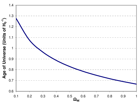
Figure 1 illustrates the relationship between the age of the Universe and for a flat Universe where .
Distance estimates from SN Ia light curves are derived from the luminosity distance
| (5) |
where and are the SN’s intrinsic luminosity and observed flux, respectively. In Friedmann-Robertson-Walker cosmologies, the luminosity distance at a given redshift, , is a function of the cosmological parameters. Limiting our consideration of these parameters to the Hubble constant, , the mass density, , and the vacuum energy density (i.e., the cosmological constant), the luminosity distance is
| (6) |
where , and is for and for , and
| (7) |
For in units of Megaparsecs, the predicted distance modulus is
| (8) |
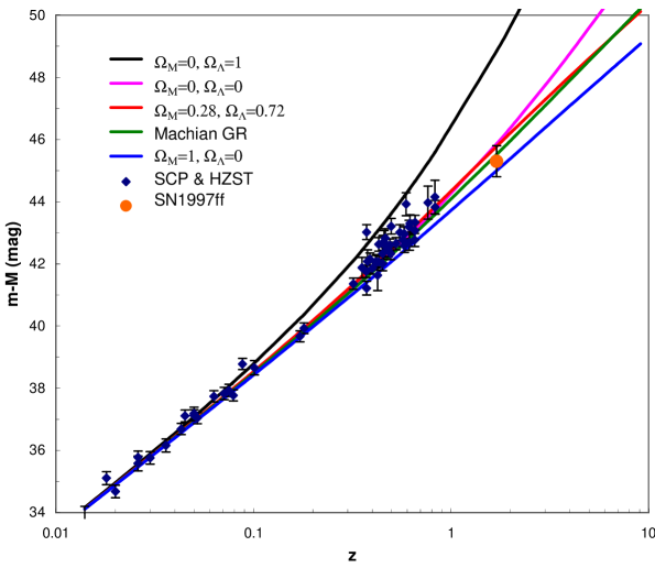
The observational dataset is illustrated in Figure 2, together with distance/redshift plots for a number of alternative cosmologies with varying and . Results from the various studies appear to provide unambiguous evidence that the Universe is accelerating, at least in comparison to a cosmological model dominated by . The best fit, based on a model with , is a Universe with and . These values also give an age for the Universe of 15 Gyr, which is in accordance with estimates from other dating methods.
1.2.3 Cosmic Microwave Background
Recent observations of the CMB [12, 22, 8, 9] have measured a peak in the power spectrum at . This provides strong evidence for a flat Universe, with . The position and amplitude of subsequent peaks at are consistent with a cosmological model having and , and a baryon energy density of , although there is considerable degeneracy between and .
1.2.4 SN 1997ff
Measurements of the luminosity-redshift relationship for merely indicate a deviation from a standard matter-dominated unverse, and are not able to distinguish between various alternative cosmological models. In order to narrow down the range of possibilities it is necessary to extend observations to include supernovae with redshifts significantly greater than one. The serendipitous discovery of SN 1997ff [5], the farthest supernova currently known, has provided the first opportunity to examine the redshift-distance relationship for cosmological bodies with ages of the order of 10 Gyr. Photometric measurements of this supernova show that it has a redshift: , and a distance modulus with a likelihood function centered around , and 95% confidence limits of and . Figure 3 shows the redshift and distance data from the SNe Ia measurement programmes, plotted together with the predictions from a number of possible cosmological models. The redshift and distance for SN1997ff is shown in relation to these models. The data and models in this figure are plotted as a delta from a linearly expanding Universe.
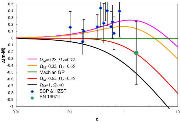
Although it is not valid to base any detailed analysis on a single data point, certain qualitative conclusions can be drawn from the SN1997ff result. The magnitude likelihood function still allows for the possibility of either a conventional decelerating Universe with , or a Universe containing dark energy with the parameters that provided the best fit based on previous SN Ia data, i.e. . However, the case does not fit with data from supernovae having , and there is only a low probability of a dark energy scenario being consistent with the SN1997ff result if . A better fit with the SN1997ff data can be obtained with and . However, these parameter values give an age for the Universe of about 12.5 Gyr, which is inconsistent with other independent estimates.
Figure 3 also shows a plot for a flat, empty Universe, with . Substituting these values in (6) gives
From Equation 2, the age of this Universe is given by
This describes a linearly expanding Universe, with an age of 15.6 Gyr, based on a current value for of . This model gives a predicted distance modulus of at a redshift , which coincides with the highest probability region of the magnitude likelihood function for SN1997ff. This model also exhibits the observed dimming behavior in comparison with a matter-dominated decelerating Universe for , albeit to a lesser extent than models with . Clearly we do not live in an empty Universe, so at first sight this model would appear to be of little use in describing a real Universe. However, we shall see in the following section that it is possible to construct an alternative cosmology that mimics the behaviour of an empty Universe, and yet has an energy density equivalent to the critical value without the need for a non-zero cosmological constant.
It is of interest to note at this point another apparent fine tuning problem in addition to the problems discussed in Section 1.1. The currently favored values for and , based on a best fit with supernova data for , are also the values which result in an age for the Universe which is in accordance with other independent estimates. These values are also very close to the values required for (see Figure 1). This may be purely coincidence, but if not, some additional fine tuning mechanism would be required to cause the ratio to take on the precise value necessary to mimic the behaviour of a linearly expanding Universe in which .
2 Machian General Relativity
2.1 Rationale for change
Before examining possible modifications to General Relativity that might give rise to alternative cosmologies, it is perhaps worthwhile considering the rational for changing what is, by any standards, a highly successful theory that has been extensively verified by numerous experiments. Arguably, from a theoretical perspective, the most compelling reason for seeking an alternative to the existing Einstein Field Equations is that General Relativity stands alone amongst gauge field theories in not being scale-invariant. This fact has motivated attempts by many workers to develop a scale-invariant theory of gravity. These have taken various forms, most notably the scalar-tensor theories first proposed by Brans and Dicke [3]. Other formulations have also been proposed, including the scale-covariant theory of Canuto [28, 27], and the conformal gravity of Mannheim [24]. The scale dependency inherent in General Relativity leads to an apparently fundamental scale, defined by the Planck units:
Planck Length
| (9) |
Planck Time
| (10) |
Planck Mass
| (11) |
No theory of Quantum Gravity is yet able to explain the wide disparity between the Planck scale and the atomic scales that govern the everyday world we inhabit. Whilst the magnitude of the Planck length and time scales, at of the corresponding atomic length and time scales, are just about reconcilable with the concept of an evolving quantum Universe, it is difficult to account for the fact that the Planck mass is times larger than the proton mass.
Cosmology presents another set of reasons for considering modifications to General Relativity. In Section 1.1 the problems associated with Big Bang cosmology were reviewed. Whilst these can be explained to an extent by concepts such as inflation and dark energy, these solutions actually raise as many problems as they solve. The Big Bang model is a direct consequence of Friedman-Robinson-Walker cosmology, which in turn is derived from the field equations of General Relativity. If a more elegant solution is to be found to the problems currently associated with the Big Bang model, then it may well be necessary to address this at source.
Finally, it can be argued that the presently accepted formulation of General Relativity leads to problems at small scales and high energies, which can only be resolved by an as-yet undiscovered theory of Quantum Gravity. The most significant manifestation of this problem is the apparent inevitability of singularities associated with Black Holes and the Planck epoch at the origin of the Universe.
2.2 Mach’s Principle
Mach’s Principle, in its most basic form, asserts that the inertia experienced by a body results from the combined gravitational effects of all the matter in the Universe acting on it. Although a great admirer of Mach, Einstein was never entirely certain whether General Relativity incorporated Mach’s Principle. Indeed, the issue is still the subject of continued debate even today (see [14] for example). A stronger version of Mach’s Principle can be formulated, which states that the inertial mass energy of a matter particle is equal and opposite to the sum of the gravitational potential energy between the particle and all other matter in the Universe, such that:
| (12) | |||||
| (13) |
where is the gravitational radius of the Universe, and is a dimensionless constant. In the case of a homogeneous and isotropic matter distribution this becomes
| (14) |
where is the average matter density of the Universe.
Observational evidence suggests that the relationship is valid to a reasonable degree of precision in the present epoch. It would be particularly satisfying if this relationship were to be found to be true, as it would tie in with the concept that the Universe is ‘a free lunch’, i.e. all the matter in the Universe could be created out of nothing, with a zero net energy. However, it can readily be seen from (14) that as the Universe continues to expand, the energy arising from gravitational attraction will ultimately tend towards zero. Conversely, gravitational energy will become infinite at , the initial singularity. Since there is no suggestion that the rest mass energy associated with the matter in the Universe changes over time (unless one is considering the Steady State Theory), it would appear that this neat zero energy condition in the present era is just a coincidence.
It can also be seen that the integral in (13) will tend towards infinity in regions of space where the gravitational field strength becomes very high, e.g. in the vicinity of a Black Hole. In order for Mach’s principle to apply not just in the present epoch, but for all time and over all space, we would have to forego the concept of a fixed Newtonian gravitational constant. Accordingly, we use (14) to derive an expression for
| (15) |
2.3 Einstein field equations revisited
Arguably Einstein’s key insight in his original formulation of the field equations of General Relativity was the postulate that space-time could be curved by the presence of energy, together with the principle of general covariance. This leads to the construction of the Einstein curvature tensor from components of the Riemann tensor:
The relationship between the Einstein curvature tensor and the stress-energy tensor is then given by:
where is a scalar ‘constant’ that determines the extent to which a given amount of stress-energy is able to curve space-time. The requirement that this should produce results that are compatible with Newtonian gravity, in the limit of weak, slowly varying gravitational fields, leads to the formulation of the full Einstein field equation:
| (16) |
The traditional cosmological constant term has been omitted from this equation. It will be shown that the observed dynamical behaviour of the Universe can in fact be explained with .
Whilst the inclusion of in the Einstein equation has the desired effect of achieving compatibility with Newtonian gravity, it could be said that in ‘writing in’ the Newtonian gravitational constant in this way, Einstein missed the opportunity to make a clean break with Newtonian gravity and to offer a more fundamental derivation for the observed scale of space-time curvature generated by stress-energy.
We are therefore looking for a formulation for the gravitational field equations that preserves the essential form of the curvature and stress-energy tensors, and yet incorporates Mach’s principle at a fundamental level. This suggests the following postulate
Postulate 1
The curvature of spacetime in a given region of the Universe, relative to a surrounding region, is proportional to the ratio of the stress-energy density in that region to the stress-energy density in the surrounding region.
In this context, the Universe is defined as being the volume of spacetime encompassed by a 3-sphere with a radius equal to the speed of light times the age of the Universe. We now take the key step of asserting that the Machian energy condition should be valid for any spacetime coordinate. Replacing the gravitational constant in (16) with the expression for in (15), leads to a redefinition of the gravitational field equation
| (17) |
where is the effective gravitational mass density, defined as
| (18) |
The geometrical constant in (15) must take the value for compatibility with Newtonian gravity and GR.
2.4 Cosmic dynamics
The components of the Einstein tensor are derived from the Robertson-Walker metric in the usual way to give
| (19) | |||||
| (20) |
The equations of motion are derived by combining (19,20) with the corresponding 00 and 11 components of the modified field equation (17) to give
| (21) | |||||
| (22) |
Since is small in the present epoch, (22) becomes
| (23) |
and (21) simplifies to
| (24) |
From this equation it can be seen that when , and the curvature , the result is a pseudo-static solution similar to the Einstein-DeSitter model, in that it has zero net energy and . The solution is pseudo-static in that the Universe is only flat and static in a cosmological reference frame. In regions of matter concentration where , will effectively appear to be zero and the Universe will therefore appear to be expanding to an observer in this reference frame, with its horizon receding at the speed of light.
This equation also embodies the negative feedback mechanism that ensures that will always be equal to . If at any point should exceed then this will lead to a positive , which will tend to drive . The converse will apply if should fall below .
2.5 Energy-momentum conservation
One of the defining features of the Einstein gravitational field equation (16) is the fact that both sides of the equation are symmetric, divergence-free, second rank tensors. The stress-energy tensor embodies the laws of energy and momentum conservation, such that . However, at fist sight the RHS of the modified field equation in (17) would appear not to be divergence-free in that the expression that replaces the gravitational constant seems to be time dependent, i.e.
| (25) |
It would seem that either we have to forego the divergence-free nature of the original Einstein equation, or we have to ‘adjust’ the new equation in some way in order to retain this desirable property. The latter approach was used in the Brans-Dicke scalar-tensor theory, and subsequently in the Canuto scale-covariant theory. Although these fixes solved the immediate problem by restoring the zero-divergence property, this was done at the expense of the overall elegance of the solution, and ultimately its ability to make any useful predictions.
How, then, are we to resolve this issue whilst still retaining the logical Machian form of the revised equation (17)? The proposed solution turns out to be both simple, and yet far reaching in terms of its potential impact. It is to redefine the nature of time within General Relativity and Quantum Mechanics.
2.6 Scale time
In order to preserve the principle of general covariance, and still retain the features of the gravitational field equations in (17) we introduce the concept of scale time, , defined as
| (26) |
where is the scale factor. Scale time is closely related to conformal time , with
| (27) |
If the Machian gravitational field equations are to exhibit the desired momentum conservation properties, we must assert that scale time is in fact the correct definition of time to use in General Relativity. Accordingly, we substitute for in (25) with , where is the time in atomic time units. Since , we see that the expression in (25) is invariant with respect to , and hence possesses zero divergence.
The concept of scale time is perhaps best visualised by considering the Universe to have the topology of a Euclidean 3-sphere, in which spatial position is defined in the usual way by three angles in spherical polar coordinates, and time corresponds to the radius of the sphere. In this model, the concepts of past, present and future do not have any real meaning. Time is merely a coordinate that determines the volume of spacetime currently occupied by a particle or field. This is in contrast to the conventional concept of spacetime embodied in a Lorentz-de Sitter metric, in which time is perceived to flow from a well defined origin in the past towards an infinite future. Scale time, as defined here, is essentially similar to the concept of imaginary time used in some descriptions of Quantum Gravity.
This leads to a somewhat bizarre picture of time and space. From the perspective of an observer in the cosmological reference frame the Universe would appear to be static and closed. Any concentrations of matter in the Universe would appear to be shrinking in size. For an observer, such as ourselves, linked to the atomic reference frame, the Universe will appear to be flat and expanding, with the horizon receding at the speed of light. Our perception of time as a continuum is an illusion, and the time co-ordinate that we are used to is perhaps better described as subjective time. For an observer in some intermediate reference frame, for example a photon that was emitted at some time in the past, the picture will be a mixture of the two scenarios described above: the Universe as a whole will appear to be expanding, but matter particles will appear to be contracting. (This notion is not entirely novel; something similar was proposed by Jeans in 1931 [18]).
The concept of two kinds of time - cosmological time and atomic time - is similar in some respects to the dual timescales postulated by Milne in his kinematic theory of gravity [4]. The important difference is that in the Machian model, only scale time is consistent with General Relativity. All other timeframes are in a sense measurements of subjective or emergent properties linked to a particular physical reference frame - in our case, one based on atomic matter. Such reference frames are not in any way unique, and one could readily conceive of a alternative reference frame based, for example, on photon time.
3 Consequences
In this section we examine the implications of the cosmological model described in Section 2 in terms of its ability to solve the Big Bang problems posed in Section 1.1, and to offer a reasonable explanation for the observed behaviour of the Universe. Throughout most of this section we shall be evaluating the effects of the model from the perspective of an observer in the atomic reference frame. Under such circumstances it will be appropriate to use the time-varying gravitational ‘constant’ formulation, with , where is the conventional (i.e. subjective) time.
3.1 Solving the Big Bang problems
3.1.1 The flatness problem
The dynamical equations in Section 2.5 clearly show that, for the Universe as a whole, the mean energy density is maintained at the critical value by a form of negative feedback mechanism. Under such circumstances, any small deviation of from unity would result in an apparent acceleration or deceleration of the expansion rate so as to bring the system back to its equilibrium state. The critical energy density of the Universe is given by
| (28) |
Using the expression for in (15) we find that
| (29) |
Recognizing the fact that Postulate 1 inevitably results in a Universe where , we shall use the terms ‘Omega model’ or ‘Omega paradigm’ as a shorthand for referring to this formulation in the following discussion.
3.1.2 The horizon problem
The Omega model requires the Universe to be spatially closed, with the topology of a 3-sphere. Because the expansion rate is constant, such that , the horizon distance will always be equal to the radius of the 3-sphere that defines the observable Universe. As a result of this coincidence of horizon distance and the radius of the observable Universe, all regions within the Universe will have been in causal contact with each other at some point in time. This accounts for the observed homogeneity of the Universe, and provides an elegant solution to the horizon problem.
The smoothness problem, i.e. accounting for the perturbations in matter density that give rise to structure formation, is not explained directly by the Omega model. As will become apparent in Section 4, the model suggests alternative scenarios for the earliest stages of cosmic evolution that may involve a boson fermion phase transition. Such transitions would result in a Universe of virtually absolute uniformity. The variations in matter density that are required as a prerequisite for galaxy structure formation must therefore arise from statistical decay processes.
3.1.3 The cosmological constant problem
This problem is resolved in the Omega model by removing the requirement for a cosmological constant altogether. It was shown in Section 1.2 that the experimental evidence for the apparent acceleration in the expansion of the Universe is consistent with a linearly expanding Universe model. In Section 2.4 we saw that the modified field equations of Machian GR give rise to just such a linear expansion. Since there is no theoretical or experimental requirement for a non-zero , it can validly be omitted from the gravitational field equations. Hence the problem of how to explain a small, but non-zero, disappears.
3.2 The Large Number Hypothesis
A dimensionless quantity known as gravitational structure constant can be defined as the ratio of the electrostatic forces between two adjacent charged particles, e.g. protons, to the gravitational force between the particles.
| (30) |
Standard cosmological theories provide no obvious explanation for such a vast disparity between the forces of gravity and electromagnetism. In 1938 Dirac [23] noted that the dimensionless quantity was approximately equal to the present age of the Universe measured in atomic time units (where 1 atomic time unit = secs). If this relationship were to be valid for all epochs then this implies that must be proportional to the age of the Universe, and therefore that . This postulate formed the basis of Dirac’s Large Number Hypothesis (LNH), which has subsequently provided the inspiration for a number of alternative cosmological theories. (It is worth noting that this formulation of the LNH is equivalent to the expression of Mach’s principle).
Clearly, since Mach’s principle has been used to construct Postulate 1, which in turn forms the basis for formulating the revised gravitational field equations, the Omega model will inherently embody the strong version of Mach’s principle. Specifically, the rest mass energy of all matter in the Universe will be equal and opposite to its mutual gravitational potential energy, such that the sum of these energies is equal to zero.
In looking at some of the implications of this relationship for observers in the atomic reference frame it is helpful to express the mean gravitational energy density of the Universe in terms of the baryon number , and the mean baryon mass, which we shall take to be the proton mass . (Note that this implies, but does not require, that any missing mass in the Universe is baryonic in nature rather than in the form of other more exotic entities).
| (31) |
The expression for in (15) can therefore be written as
| (32) |
If we now substitute for in equation (30) for the gravitational structure constant , we find that
| (33) |
where is the apparent radius of the Universe in the atomic reference frame, at subjective time . From this it can be seen that in our reference frame, i.e. the strength of the gravitational interaction between particles will increase over time in relation to their mutual electromagnetic forces. Combining (33) with the expression for atomic time we find that
| (34) |
where is the time in atomic time units. Although this very simple result may at first seem somewhat surprising, it is perhaps to be expected, since the baryon number is one of the few dimensionless quantities to occur naturally in cosmology. (The fact that today is purely a coincidence). The implications of the time dependence of for will be examined in Section 4.
3.3 Planck Units
We shall now examine the effects of recasting the expressions for the Planck units using the formula for given in (32), and the de Broglie wavelength of a proton given by .
Planck Length
Clearly with the quantity known as the Planck Length in (9) will itself be a function of time such that . Substituting for using (32), and the expression for the atomic time unit, gives
| (35) |
where is the time expressed in atomic time units, and is the baryon number of the Universe. It is interesting to note that at a time the Planck Length will have grown to a size such that . (Or conversely, in the cosmological frame, the proton wavelength will have shrunk below the Planck Length). The implications of this equality for the ultimate fate of the Universe will be revisited in Section 4.
Planck Time
A similar set of expressions can be derived for the quantity known as Planck Time in (10), to give
| (36) |
Planck Mass
From Equation (11) it is evident that the Planck Mass . Again, substituting for using (32), with we find
| (37) |
And when we see that . It is easy to verify that these expressions lead to the correct present day values for the Planck units by inserting appropriate values for the proton mass and radius, and the current time in atomic time units.
Based on this analysis, the conclusion we must reach is that Planck Units do not represent a fundamental measurement scale that becomes relevant during the birth of the Universe and governs the realm of Quantum Gravity. Rather, they are scale factor dependent quantities which may shed some light on the behaviour of the Universe in its dying moments.
3.4 Cosmological observations
We have already seen in Section 2.4 that a linearly expanding Universe, such as the one that would evolve from the modified gravitational field equations, will give rise to the currently observed Universe, with:
-
•
Hubble parameter for a Universe of age .
-
•
Critical density
-
•
Apparent acceleration relative to a Universe with
3.5 Variations in the gravitational constant
The prediction that , where is the scale factor, is another principal feature of the Omega model. However, it will not be possible to detect any variation in by, for example, measuring changes in planetary orbits within the solar system using radar ranging techniques, since time measured by any atomic or gravitational clock will be changing at the same rate as the distance to be measured. Suppose at time and scale factor the measured distance is , where is the period of an atomic clock and is the number of clock ticks between the emission of a radar signal and the reception of its reflection. At some future time when the scale factor has increased to , the measurement is repeated. If then the distance to the planet will have decreased so that . However, the period of the atomic clock will also have decreased by the same proportion, with . Consequently, the measured elapsed time for the radar signal round trip will still be ticks, i.e. there will be no apparent change in distance and therefore no change in gravitational constant.
In order to verify that does vary over cosmological timescales it will be necessary either to measure its value directly using a Cavendish type experiment, or to turn to evidence from geophysical and astrophysical measurements, and from models of galactic evolution. Since Cavendish experiments can currently only achieve accuracies of one part in , these are not capable of detecting changes in , which will be of the order of the Hubble factor, i.e. one part in per year. We must therefore look to the other sources for indirect evidence of a time-varying .
3.6 Varying Speed of Light Cosmology
A novel cosmology, based on the concept of a varying speed of light, has been proposed by Albrecht, Barrow, and Magueijo ([1, 16, 17, 15]). This is capable of explaining the Big Bang problems by postulating that, at an epoch corresponding approximately to the inflationary era in the standard Big Bang plus inflation model, the speed of light was much greater than it is today. In the Omega model, the fact that means that the velocity of light, , must be constant as measured by an observer at scale factor . However, it is easy to see that if an observer had some means of measuring conventional time, rather than subjective time derived from scale time, then they would perceive a steady decrease in the speed of light with time. In other words, a linearly expanding Universe consistent with Machian GR is equivalent to a static Universe in which the speed of light varies.
4 Predictions
As with any other theory, the usefulness of the Omega paradigm hinges on its ability not only to explain currently observed phenomena, but also to successfully predict new phenomena which can subsequently be verified by experiment. It has already been shown in Section 3 that the Omega model can provide explanations for some of the problems associated with the standard Big Bang model that are considerably more economical than other prevailing theories. Similarly, it has provided a logical explanation for the presently observed values of a number of fundamental physical quantities. In this section we use the underlying features of this model to make several predictions pertaining to the history and the fate of the Universe.
4.1 Photon energy conservation
The concept of scale time, which is an essential component of the Omega model, necessitates a reappraisal of the way in which the equivalence principle is applied in General Relativity. Essentially, the notion of time as a linear flow of events with a past, present and future, must be replaced by a picture of time as a fourth dimension of finite extent. Scale time is a measure of the proportion of this time dimension that is occupied by a particle or field. With this formulation of time it is evident that there is no preferred ‘position’ in the time dimension, any more than there is in the three spatial dimensions. One can, of course, still define specific reference frames in which to carry out physical measurements, the most obvious being the atomic reference frame that we use for most everyday purposes.
Extending the equivalence principle to embrace this concept, its is clear that the Hamiltonian of a system should be independent of the choice of time co-ordinate. This presents little conceptual difficulty when applied to a system of particles or bound fields. However, when the principle is extended to photons it is hard to escape the conclusion that the energy of a photon must be independent of the reference frame of the observer. In other words, photons will retain the same energy that they originally possessed at the time of their emission, whether they are red-shifted (or blue-shifted) as a result of
-
•
Doppler shift with respect to a given observer
-
•
climbing out of a gravitational potential
-
•
being ‘stretched’ by the Hubble expansion of the Universe
The observable quantity that will change in the reference frame of the observer will be the power of the photon.
Clearly, if this prediction is valid then it would have fundamental implications across many fields of physics. However the effects should be experimentally verifiable. In the field of cosmology, the most obvious place to look for evidence of photon energy conservation is in the cosmic microwave background (CMB). The standard theory is based on the assumption that as the Universe expands, the energy density due to matter decreases as , whereas the energy density due to radiation decreases as because of the additional energy loss due to the red-shift. In the Omega model this remains true when looking at the spatial energy density. However, if one is carrying out measurements of photon energy by integrating power measurements over a period of time that is long in relation to the time span of the photon wavepacket (i.e. ), then the energy will be found to decrease in proportion to , as for the matter case. So, for example, a CMB photon emitted when the Universe had a temperature of , with a present day temperature of , would still retain its initial energy given by , rather than of this value.
It should in theory be possible to measure this effect experimentally, by analysis of the noise spectrum of the CMB. Most recent experiments to measure the CMB have focused on obtaining improved spatial resolution in order to map out temperature fluctuations, and hence matter distribution, in the early Universe. This has necessitated integrating microwave power measurement over timescales that are long enough to achieve an adequate CMB signal against the background noise level. An experiment to measure the CMB noise spectrum will need to have a much narrower time resolution (), but conversely, the measurement can be integrated over a much larger solid angle. The standard theory predicts that the results of a Fourier analysis of these measurements will be a constant noise power level over the entire frequency range, up to the cut-off determined by the sampling time window. The Omega model predicts that the noise power spectrum will be in the form of a Gaussian distribution, with the peak of the distribution corresponding to the mean CMB photon arrival rate.
4.2 Primordial nucleosynthesis
Arguably, one of the few successes of the standard Big Bang model is its ability to predict the abundances of the light elements resulting from primordial nucleosynthesis. If the Omega model is to be of any use then it must also give predictions that are consistent with observational data. The Omega model implies that the observed power of the CMB is due to a relatively small number of energetic photons rather than a very large number of low energy photons. Assuming that the CMB photons originally had energies of , corresponding to a temperature of . These have been redshifted to the currently measured temperature of , implying an energy loss of the order of according to the standard theory. Since the currently observed CMB photon number density, calculated according to the standard theory, happens to correspond to photons per baryon, it follows that in the Omega model.
The current CMB photon energy density is approximately of the observed energy density due to baryonic matter. Taking these two observations together, this suggests that we are looking for a nucleosynthesis model that results in one photon per baryon, with an energy approximately of the proton rest mass energy. The most obvious scenario is that of neutron decay, first proposed by Gamow [13]. Initial studies of the evolution of a cold neutron Universe have been carried out using numerical simulation models. These show that the initially cold, dense, neutron cloud heats up by means of decay to form a hot proton-neutron-electron plasma at a temperature of . At a range of fusion reactions become energetically favorable, and lead to the formation of deuterium, tritium, helium and other light elements, as in the standard Big Bang nucleosynthesis models [25]. The main differences between the Omega model and the standard Big Bang is that in the former, photons play a negligible role in the exchange of energy between particles. The fact that the expansion rate is much slower also has a significant impact in that there is more time for fusion reactions to take place, and therefore an increased probability of synthesizing heavier elements than would be the case with the standard model. Nucleosynthesis in a linearly expanding Universe has also been studied by Lohiya in [6].
One of the most important consequences of nucleosynthesis in the Omega model is that the primordial baryonic matter is not able to cool down as the Universe expands, since there are insufficient photons to remove the entropy generated by the neutron decay and nuclear fusion processes. The primordial hydrogen and helium molecules will therefore remain in an ionized state indefinitely. This may explain why intergalactic gas clouds are currently observed to be ionized. Another feature of this model is that the decay process that causes the primordial universe to heat up will give rise to scale-invariant differences in temperature, due to the statistical nature of the neutron decay reaction. Starting from a perfectly isotropic and homogeneous state, this mechanism is therefore able to account for the observed scale-invariant temperature fluctuations in the CMB, which are explained by inflation in the standard Big Bang model.
4.3 Black Holes and singularities
The modified gravitational field equation in (17) is only valid where the matter density is homogeneous and isotropic. In the more general case where , it is necessary to use the full version of the modified field equation
| (38) |
From this it can be seen that in regions of high energy density, such as the vicinity of a Black Hole, the density integral will be much larger than its average value for the Universe as a whole. The resulting curvature due to stress-energy in will therefore be proportionately less than it would be in regions of average matter density. As an example of the consequence of this phenomenon, consider two stars orbiting in close proximity to a Black Hole. Under conventional GR, the mutual gravitational attraction between these two bodies would be given by the standard Einstein gravitational equation. With Machian GR, the additional curvature induced in the metric as a result of the mass of each of the stars will tend towards zero as they approach the Swartzchild radius of the Black Hole. Expressed in terms of a simple mechanical analogy, we could say that spacetime becomes stretched to its elastic limit in the vicinity of a Black Hole, to the extent that the presence of additional mass-energy is not able to increase curvature any further.
A further consequence of Machian GR is that if Postulate(1) holds true under all circumstances, then it follows that as matter passes through the event horizon of a Black Hole, it enters a region of spacetime that is effectively a separate Universe from the one that exists outside the Black Hole. Under such circumstances, all dimensions are rescaled, and there is no central singularity.
4.4 Implications for Quantum Gravity
The discussion of the scale factor dependency of the gravitational structure constant and the Planck units leads to the conclusion that the conditions applying in the very early Machian GR Universe would bear little resemblance to the scenario envisaged in the standard Big Bang model. Specifically, the Penrose-Hawking singularity theorem [26], which is predicated on a conventional concept of time and gravity, would no longer apply under the Omega model. In fact the proto-Universe would be a much more benign environment, without any initial singularity as such. In the absence of an initial singularity, there is no need to resort to the concept of a cut-off point occurring at the Planck length and time. In any case, we have seen that in the Omega model these quantities are themselves time dependent, and do not therefore carry the same fundamental significance that is attached to them in the standard theory. The existence the singularity at the Planck era is one of the two principle motivations for the pursuit of a quantum theory of gravity (the other being the need for the curvature terms in the gravitational field equation to be quantized in order to be equivalent to the stress-energy terms). If this factor is removed, we need to ask whether there is still a need for a theory of Quantum Gravity, at least in the form currently being sought.
In Section 2.6, an alternative spacetime structure was described, which potentially allows processes to occur ’simultaneously’, but at different time coordinates. This has a number of implications, including the possibility that several particle ’generations’ can coexist within the Universe, each at a different stage in their time evolution. This might conceivably provide an explanation for the missing mass problem, which incidentally is not addressed by the Omega model. The spacetime structure also offers the intriguing possibility that processes operating in the cosmological reference frame, i.e. across the whole Universe, can occur in the same time as local processes occurring in the atomic reference frame. If this were to be the case, then it provides a mechanism for explaining the apparent paradox of action-at-a-distance and non-locality associated with Quantum Mechanics.
4.5 The ultimate fate of the Universe
In Section 3 we saw that at a time (where is the time in atomic time units, and is the baryon number of the Universe), the evolution of the Omega Universe reaches a state at which the Planck length is equal to the Compton wavelength of the proton, and the Planck mass is equal to the proton mass. Recalling that the Schwartzchild radius of a black hole is given by
| (39) |
and substituting for using (32), with and , we find that
| (40) |
In other words, the scale factor of the Universe has evolved to the point where the radius of the proton exceeds the Schwartzchild radius corresponding to the proton mass. (The term proton here is used loosely to refer to whatever state baryonic matter may exist in the extreme gravitational conditions prevailing at this epoch. In practice it is more likely that protons and electrons will have recombined into atomic hydrogen by this stage, which in turn may have collapsed into neutrons in a reversal of the process described in 4.2 above). At this point the Universe effectively comes to an end as all protons simultaneously collapse into micro Black Holes - possibly to give birth to many more baby Universes according to Smolin in [21].
References
- [1] A.Albrecht and J.Magueijo. a time varying speed of light as a solution to cosmological problems. astro-ph, 9811018.
- [2] A.G.Reiss. observational evidence from supernovae for an accelerating universe and cosmological constant. astro-ph/9805201, 1998.
- [3] C.Brans and R.Dicke. Mach’s principle and a relativistic theory of gravity. Physical Review, 124:925–935, 1961.
- [4] E.A.Milne. Kinematic relativity. Proc. R. Soc. A, 165:351, 1938.
- [5] A.G.Reiss et al. the farthest known supernova: support for an acelerating universe and a glimpse of the epoch of deceleration. astro-ph/0104455, 2001.
- [6] D.Lohiya et al. Nucleosynthesis in a simmering universe. gr-qc/9808031, 1998.
- [7] M.Hamuy et al. the absolute luminosities of the Calan/Tololo Type Ia supernovae. Astrophysical Journal, 112:2391, 1996.
- [8] P.de Bernardis et al. a flat universe from high-resolution maps of the cosmic microwave background radiation. Nature, 2000.
- [9] P.de Bernardis et al. multiple peaks in the angular power spectrum of the cosmic microwave background: significance and consequences for cosmology. astro-ph/0105296, 2001.
- [10] S.Perlmutter et al. cosmology from type 1a supernovae. astro-ph/9812473, 1998.
- [11] S.Perlmutter et al. measurements of and from 42 high redshift supernovae. astro-ph/9812133, 1998.
- [12] G.Efstathiou. CMB anisotoropies and the determination of cosmological parameters. astro-ph/0002249, 2000.
- [13] G.Gamow. Evolution of the universe. Nature, 162:680–2, Oct 1948.
- [14] J.Barbour and H.Pfister. From Newton’s Bucket to Quantum Gravity. Birkh user, 1995.
- [15] J.D.Barrow and J.Magueijo. solutions to the quasi-flatness and quasi-lambda problems. astro-ph/9811073, 1998.
- [16] J.D.Barrow and J.Magueijo. varying- theories and solutions to the cosmological problems. astro-ph/9811072, 1998.
- [17] J.D.Barrow and J.Magueijo. solving the flatness and quasi-flatness problems in brans-dicke cosmologies with a varying light speed. astro-ph/9901049, 1999.
- [18] J.Jeans. Evolution of the universe. Nature, 128:703, 1931.
- [19] J.Magueijo and K.Baskerville. Big bang riddles and their revelations. astro-ph/9905393, 1999.
- [20] L.Bergstrom and A.Goobar. Cosmology and Particle Astrophysics. Wiley, 1999.
- [21] L.Smolin. The fate of Black Hole singlularities and the parameters of the standard models of particle physics and cosmology. gr-qc/9404011, 1994.
- [22] M.White, D.Scott, and E.Pierpaoli. Booomerang returns unexpectedly. astro-ph/0004385, 2000.
- [23] P.A.M.Dirac. The large number hypothesis. Proc.R. Soc. A, 165:199, 1938.
- [24] P.Mannheim. conformal cosmology with no cosmological constant. Gen. Relativ. Gravit., 22:289, 1990.
- [25] R.V.Wagoner, W.A.Fowler, and F.Hoyle. Primordial nucleosynthesis. Ap.J., 148:3, 1967.
- [26] S.W.Hawking and R.Penrose. The singluarities of gravitational collapse and cosmology. Proc. Roy. Soc. London, A314:529, 1970.
- [27] V.Canuto, H.S.Hsieh, and P.J.Adams. Mach’s principle, the cosmological constant, and the scale-covariant theory of gravity. Physical Review D, 18(10):3577, 1978.
- [28] V.Canuto, P.J.Adams, S.H.Hsieh, and E.Tsiang. Scale-covariant theory of gravitation and astrophysical applications. Physical Review D, 16(6):1643, 1977.