On Radar Time and the Twin ‘Paradox’

Abstract

In this paper we apply the concept of radar time (popularised by Bondi in his work on k-calculus) to the well-known relativistic twin ‘paradox’. Radar time is used to define hypersurfaces of simultaneity for a class of travelling twins, from the ‘Immediate Turn-around’ case, through the ‘Gradual Turn-around’ case, to the ‘Uniformly Accelerating’ case. We show that this definition of simultaneity is independent of choice of coordinates, and assigns a unique time to any event (with which the travelling twin can send and receive signals), resolving some common misconceptions.

INTRODUCTION

It might seem reasonable to suppose that the twin paradox has long been understood, and that no confusion remains about it. Certainly there is no disagreement about the relative aging of the two twins, so there is no ‘paradox’. There is also no confusion over ‘when events are seen’ by the two twins, or over the description by the stay-at-home twin (Alex say), of ‘when events happened’. These aspects of the twin paradox are treated in the standard texts${}^{\mbox{\scriptsize\cite[cite]{[\@@bibref{}{Bohm,Dinverno,Leo,Pauli}{}{}]}}}$.

However, the description of ‘when events happened’ according to the travelling twin (Barbara say) seems never to have been fully settled${}^{\mbox{\scriptsize\cite[cite]{[\@@bibref{}{Unruh2,Debs}{}{}]}}}$. In textbook treatments, Barbara’s hypersurfaces of simultaneity, which define ‘when events happened’ according to her, have consistently been misrepresented or ignored. A common diagram for such hypersurfaces${}^{\mbox{\scriptsize\cite[cite]{[\@@bibref{}{Bohm,Dinverno,Leo,Debs}{}{}]}}}$ is shown in Figure 1.

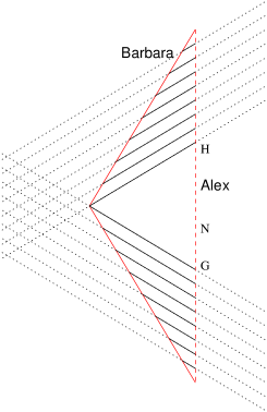
Figure 1: A typical ‘textbook illustration’ of the hypersurfaces of simultaneity of the travelling twin in the twin paradox.

Bohm${}^{\mbox{\scriptsize\cite[cite]{[\@@bibref{}{Bohm}{}{}]}}}$ and Sartori${}^{\mbox{\scriptsize\cite[cite]{[\@@bibref{}{Leo}{}{}]}}}$ claim that points G and H appear to the travelling twin as simultaneous, while Bohm${}^{\mbox{\scriptsize\cite[cite]{[\@@bibref{}{Bohm}{}{}]}}}$ goes on to say that “after the acceleration at E an event such as N is ascribed a smaller time coordinate than it had before”! Other authors${}^{\mbox{\scriptsize\cite[cite]{[\@@bibref{}{Leo,Dinverno}{}{}]}}}$, noticing this problem, claim that its resolution lies in an analysis of the interval that the travelling twin must take to turn around (at a finite acceleration), and that during this period of acceleration Barbara’s hypersurfaces of simultaneity ‘sweep round’ from EG to FH, as shown in Figure 2.

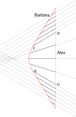
Figure 2: Another typical ‘textbook illustration’, in which Barbara’s hypersurfaces of simultaneity ‘sweep round’ from EG to FH during her period of acceleration.

Although this period of acceleration can indeed fix the gap between G and H, it cannot resolve the more serious problem (mentioned also in Marder${}^{\mbox{\scriptsize\cite[cite]{[\@@bibref{}{Marder}{}{}]}}}$ and in Misner et al.${}^{\mbox{\scriptsize\cite[cite]{[\@@bibref{}{Misner}{}{}]}}}$) which occurs to Barbara’s left. Here her hypersurfaces of simultaneity are overlapping, and she assigns three times to every event! Also, if Barbara’s hypersurfaces of simultaneity at a certain time depend so sensitively on her instantaneous velocity as these diagrams suggest, then she would be forced to conclude that the distant planets swept backwards and forwards in time whenever she went dancing!

The path through this confusion existed already in Einstein’s original paper${}^{\mbox{\scriptsize\cite[cite]{[\@@bibref{}{Ein}{}{}]}}}$, and was popularised by Bondi in his work on ‘k-calculus’. It lies in the correct application of ‘radar time’ (referred to as ‘Märzke-Wheeler Coordinates’ in Pauri et al.${}^{\mbox{\scriptsize\cite[cite]{[\@@bibref{}{Pauri}{}{}]}}}$). This concept is not new. Indeed Bohm${}^{\mbox{\scriptsize\cite[cite]{[\@@bibref{}{Bohm}{}{}]}}}$ and D’Inverno${}^{\mbox{\scriptsize\cite[cite]{[\@@bibref{}{Dinverno}{}{}]}}}$ both devote a whole chapter to k-calculus, and use ‘radar time’ (not under that name) to derive the hypersurfaces of simultaneity of inertial observers. However, both authors then apply this definition wrongly to the travelling twin.

In the present paper we recall the definition of ‘radar time’ (and related ‘radar distance’) and emphasise that this definition applies not just to inertial observers, but to any observer in any spacetime. We then use radar time to derive the hypersurfaces of simultaneity for a class of travelling twins, from the ‘Immediate Turn-around’ case, through the ‘Gradual Turn-around’ case, to the ‘Uniformly Accelerating’ case. (The ‘Immediate Turn-around’ and ‘Uniformly Accelerating’ cases are also discussed in Pauri et al.${}^{\mbox{\scriptsize\cite[cite]{[\@@bibref{}{Pauri}{}{}]}}}$.) We show that in all cases this definition assigns a unique time to any event with which Barbara can send and receive signals, and that this assignment is independent of any choice of coordinates. We then demonstrate that brief periods of acceleration have negligible effect on the radar time assigned to distant events, in contrast with the sensitive dependence of the hypersurfaces implied by Figures 1 and 2. By viewing the situation in different coordinates we further demonstrate the coordinate independence of radar time, and note that there is no observational difference between the interpretations in which the differential aging is ‘due to Barbara’s acceleration’ or ‘due to the gravitational field that Barbara sees because of this acceleration’.

RADAR TIME AND RADAR DISTANCE

Consider an observer travelling on path $\gamma:x^{\mu}=x^{\mu}_{(\gamma)}(\tau)$ with proper time $\tau$. Define:

$$\tau^{+}(x) \equiv\mbox{ (earliest possible) proper time at which a light ray}$$

(technically, a null geodesic) leaving point $$x \gamma$$ could intercept .

$$\tau^{-}(x) \equiv\mbox{ (latest possible) proper time at which a light ray}$$

(null geodesic) could leave $$\gamma x$$, and still reach point .

$$\tau(x) \equiv{\textstyle\frac{1}{2}}(\tau^{+}(x)+\tau^{-}(x))\hskip 28.45274pt=\mbox{ `radar time'.}$$

$$\rho(x) \equiv{\textstyle\frac{1}{2}}(\tau^{+}(x)-\tau^{-}(x))\hskip 28.45274pt=\mbox{ `radar distance'.}$$

$$\Sigma_{\tau_{0}} \equiv\{x:\tau(x)=\tau_{0}\}$$

$$=\mbox{ observer's `hypersurface of simultaneity at time $\tau_{0}$'. }$$

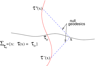
Figure 3: Schematic of the definition of ‘radar time’ $\tau(x)$.

This definition was made popular by Bondi in his work on special relativity and k-calculus${}^{\mbox{\scriptsize\cite[cite]{[\@@bibref{}{Bondi,Bohm,Dinverno}{}{}]}}}$, and is essentially a rearrangement of the formula $t-t^{-}=t^{+}-t$ from Einstein’s original paper${}^{\mbox{\scriptsize\cite[cite]{[\@@bibref{}{Ein}{}{}]}}}$ (written as $t_{B}-t_{A}=t^{\prime}_{A}-t_{B}$ in Einstein’s notation). This formula simply says that an observer can assign a time to a distant event by sending a light signal to the event and back, and averaging the (proper) times of sending and receiving. It is clearly applicable to any observer in any gravitational background. However, the idea of defining hypersurfaces of simultaneity in terms of ‘radar time’ has seldom been applied to non-inertial observers or to non-flat spacetimes. This is perhaps due to Bondi’s claim that${}^{\mbox{\scriptsize\cite[cite]{[\@@bibref{}{Bondi}{}{}]}}}$ “how a clock reacts to acceleration is utterly dependent on how the clock is constructed”. This claim has since been refuted by experiment (see ${}^{\mbox{\scriptsize\cite[cite]{[\@@bibref{}{Marder}{}{}]}}}$, or ${}^{\mbox{\scriptsize\cite[cite]{[\@@bibref{}{Dav3}{}{}]}}}$ pp 144,145, and references therein); moreover the assumption that ‘suitable clocks’ will behave identically under acceleration (or under gravitational fields) is a basic premise of general relativity, without which proper time would have no physical meaning. There is therefore no reason not to apply ‘radar time’ to accelerating observers or to curved spacetimes.

Since radar time can be defined without any mention of coordinates it is, by construction, independent of our choice of coordinates. It is single-valued, agrees with proper time on the observers path, and is invariant under ‘time-reversal’ - that is, under reversal of the sign of the observer’s proper time.

THE TRAVELLING TWIN

Consider the standard ‘Immediate Turn-around’ case, for which Barbara’s path is given by

$$(t_{B}(\tau),x_{B}(\tau))=\begin{cases}(\cosh(\alpha)\tau\ ,\ \sinh(\alpha)\tau)&(\tau>0)\\ (\cosh(\alpha)\tau\ ,\ -\sinh(\alpha)\tau)&(\tau<0)\\ \end{cases}$$

or:

$$(u_{B}(\tau),v_{B}(\tau))=\begin{cases}(e^{\alpha}\tau\ ,\ -e^{-\alpha}\tau)&(\tau>0)\\ (e^{-\alpha}\tau\ ,\ -e^{\alpha}\tau)&(\tau<0)\\ \end{cases}$$

where $s=\tanh(\alpha)$ is Barbara’s speed (in units with $c=1$), $\alpha$ is her ‘rapidity’, and we have defined coordinates $(u,v)$ by $u\equiv x+t$ and $v\equiv x-t$. This situation is shown in Figure 4 below.

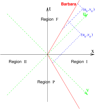
Figure 4: The travelling twin in the ‘Immediate Turn-around’ case.

To deduce the radar time of a point $(u_{0},v_{0})$, it is convenient to consider 4 different regions, depending on the signs of $u_{0}$ and $v_{0}$.

Region I: $u_{0}>0$ and $v_{0}>0$

Clearly, $\tau^{+}(u_{0},v_{0})$ is determined by putting $u_{0}=u_{B}(\tau^{+})=e^{\alpha}\tau^{+}$ (where we have used $u_{B}(\tau^{+})=e^{\alpha}\tau^{+}$ since we see from Figure 4 that $\tau^{+}>0$). Similarly, $\tau^{-}(u_{0},v_{0})$ is determined by putting $v_{0}=v_{B}(\tau^{-})=-e^{\alpha}\tau^{-}$ (since $\tau^{-}<0$). Hence:

$$\tau(u_{0},v_{0}) ={\textstyle\frac{1}{2}}(e^{-\alpha}u_{0}-e^{-\alpha}v_{0})$$

$$=e^{-\alpha}t_{0}$$ (1)

in this region.

Region F: $u_{0}>0$ and $v_{0}<0$

Consider first the case where $(u_{0},v_{0})$ is to Barbara’s right, as shown in Figure 4. The calculation of $\tau(u_{0},v_{0})$ proceeds as in the previous case, the only difference being that, since $\tau_{-}>0$, we now use $v_{B}(\tau^{-})=-e^{-\alpha}\tau^{-}$ (the exponent has changed sign). Hence we have

$$\tau(u_{0},v_{0}) ={\textstyle\frac{1}{2}}(e^{-\alpha}u_{0}-e^{\alpha}v_{0})$$

$$=\cosh(\alpha)t_{0}-\sinh(\alpha)x_{0}$$ (2)

If $(u_{0},v_{0})$ is to Barbara’s left (but still in region F) then the roles played by $\tau^{+}$ and $\tau^{-}$ are reversed, but since the definition of $\tau$ is symmetric under this change it follows that (2) remains unchanged, and holds throughout region F.

Regions II and P are treated similarly, and we find:

$$\tau(t,x)=\begin{cases}te^{-\alpha}&\mbox{ region I}\\ te^{\alpha}&\mbox{ region II}\\ \cosh(\alpha)t-\sinh(\alpha)x&\mbox{ region F}\\ \cosh(\alpha)t+\sinh(\alpha)x&\mbox{ region P}\\ \end{cases}$$

The ‘hypersurface of simultaneity at time $\tau_{0}$’, denoted $t_{\tau_{0}}(x)$ is now given by putting $\tau(t,x)=\tau_{0}$ and rearranging. This gives:

$$t_{\tau_{0}}(x)=\begin{cases}\tau_{0}e^{\alpha}&\mbox{ region I}\\ \tau_{0}e^{-\alpha}&\mbox{ region II}\\ \mbox{sech}(\alpha)\tau_{0}+\tanh(\alpha)x&\mbox{ region F}\\ \mbox{sech}(\alpha)\tau_{0}-\tanh(\alpha)x&\mbox{ region P}\\ \end{cases}$$

as shown for various $\tau_{0}$ in Figure 5.

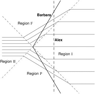
Figure 5: Hypersurfaces of simultaneity of the travelling twin in the ‘Immediate Turn-around’ case.

We now see that in region F, where Barbara is indistinguishable from an inertial observer with velocity $s$, her hypersurfaces of simultaneity are exactly those appropriate to such an inertial observer; while in region P, where she is indistinguishable from an inertial observer with velocity $-s$, her hypersurfaces are those appropriate to that inertial observer. This is not true in regions I and II however, for which she has differing velocities when she sends her signal (at time $\tau^{-}$) when she receives it back (at time $\tau^{+}$). In these regions her hypersurfaces of simultaneity are flat (as expected for symmetry under time reversal). Hence she assigns a unique time to each event, avoiding the problems that appear in the common ‘textbook illustrations’ (Fig. 1, 2).

We now consider the effect on these conclusions of a small period of acceleration at the point of turn-around.

GRADUAL TURN-AROUND

We allow Barbara to turn around at finite acceleration $a$, for a proper time $\tau_{c}=\frac{\alpha}{a}$. Barbara’s trajectory is now given by:

$$t_{B}(\tau)=\begin{cases}\cosh(a\tau_{c})(\tau-\tau_{c})+\frac{1}{a}\sinh(a\tau_{c})&(\tau\geq\tau_{c})\\ \frac{1}{a}\sinh(a\tau)&(|\tau|\leq\tau_{c})\\ \cosh(a\tau_{c})(\tau+\tau_{c})-\frac{1}{a}\sinh(a\tau_{c})&(\tau\leq-\tau_{c})\\ \end{cases}$$

$$x_{B}(\tau)=\begin{cases}\sinh(a\tau_{c})(\tau-\tau_{c})+\frac{1}{a}\cosh(a\tau_{c})&(\tau\geq\tau_{c})\\ \frac{1}{a}\cosh(a\tau)&(|\tau|\leq\tau_{c})\\ -\sinh(a\tau_{c})(\tau+\tau_{c})+\frac{1}{a}\cosh(a\tau_{c})&(\tau\leq-\tau_{c})\\ \end{cases}$$

and her final speed is $s=\tanh(a\tau_{c})$. In null coordinates this is:

$$(u_{B}(\tau),v_{B}(\tau))$$

$$=\begin{cases}(e^{a\tau_{c}}(\tau-\tau_{c}+\frac{1}{a})\ ,\ -e^{-a\tau_{c}}(\tau-\tau_{c}-\frac{1}{a}))&(\tau\geq\tau_{c})\\ (\frac{1}{a}e^{a\tau}\ ,\ \frac{1}{a}e^{-a\tau})&(|\tau|\leq\tau_{c})\\ (e^{-a\tau_{c}}(\tau+\tau_{c}+\frac{1}{a})\ ,\ -e^{a\tau_{c}}(\tau+\tau_{c}-\frac{1}{a}))&(\tau\leq-\tau_{c})\\ \end{cases}$$

We now have nine regions to consider, separated by $u=e^{\pm a\tau_{c}}$ and $v=e^{\pm a\tau_{c}}$. The calculation is straightforward, and yields hypersurfaces of simultaneity of the form:

$$t_{\tau_{0}}(x)=\begin{cases}\tau_{0}e^{\pm a\tau_{c}}&\mbox{ regions I, II}\\ \mbox{sech}(a\tau_{c})(\tau_{0}\pm\tau_{c})\mp\tanh(a\tau_{c})x&\mbox{ regions P, F}\\ x\tanh(a\tau_{0})&\mbox{ region U}\\ \end{cases}$$

while in the other 4 regions these hypersurfaces are given implicitly by:

$$\log(a|x +t_{\tau_{0}}(x)|)+a(t_{\tau_{0}}(x)-x)e^{\pm a\tau_{c}}$$

$$=2a\tau_{0}\mp a\tau_{c}-1\hskip 28.45274pt\mbox{ regions FII, PI}$$

$$\log(a|x -t_{\tau_{0}}(x)|)-a(t_{\tau_{0}}(x)+x)e^{\pm a\tau_{c}}$$

$$=-2a\tau_{0}\mp a\tau_{c}-1\hskip 19.91684pt\mbox{ regions FI, PII}$$

Figure 6: Hypersurfaces of simultaneity of the travelling twin in the ‘Gradual Turn-around’ case.

These hypersurfaces are shown in Figure 6. As hoped, there is very little difference (for small $\tau_{c}$) between the ‘Immediate Turn-around’ and ‘Gradual Turn-around’ cases. The hypersurfaces in regions I and II are identical to the previous case, while in regions F and P the only difference is that a slightly different value of $\tau_{0}$ is assigned to each hypersurface, due to the slight difference in turn-around time. This contrasts with the situation described in many textbooks${}^{\mbox{\scriptsize\cite[cite]{[\@@bibref{}{Marder,Dinverno}{}{}]}}}$ and depicted in Figure 2.

It is interesting to consider the limit $\tau_{c}\rightarrow\infty$, corresponding to a uniformly accelerating observer. In this case we have simply:

$$(t_{B}(\tau),x_{B}(\tau)) =\left(\frac{1}{a}\sinh(a\tau)\ ,\ \frac{1}{a}\cosh(a\tau)\right)$$

$$\mbox{ or }(u_{B}(\tau),v_{B}(\tau)) =\left(\frac{1}{a}e^{a\tau}\ ,\ \frac{1}{a}e^{-a\tau}\right)$$

A simple calculation yields radar time and radar distance:

$$\tau(t,x) =\frac{1}{2a}\log\left(\frac{x+t}{x-t}\right)$$

$$\rho(t,x) =\frac{1}{2a}\log(a^{2}(x^{2}-t^{2}))$$

The hypersurfaces of simultaneity are therefore given by

$$t_{\tau_{0}}(x)=x\tanh(a\tau_{0})$$

just as in region $U$ of Fig. 6.

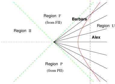
Figure 7: Hypersurfaces of simultaneity of a uniformly accelerating observer.

$\rho$ and $\tau$ are simply Rindler coordinates now, and cover only region U. This is as expected, since Barbara cannot send a signal to any events in regions P or II, while no signals could reach Barbara from regions F or II.

GRAVITY DOESN’T MATTER

It is often said of the twin paradox that${}^{\mbox{\scriptsize\cite[cite]{[\@@bibref{}{Pauli}{}{}]}}}$ “a complete explanation of the problem can only be given within the framework of general relativity”. However, as we have just shown, Barbara’s hypersurfaces of simultaneity depend only on the kinematics involved, and can be fully understood without resorting to general relativity. To understand why ‘equivalent gravitational fields’ are some times invoked in the literature, consider the ‘Uniformly Accelerating’ case, as described in $(\tau,\rho)$ coordinates. This is shown in Figure 8.

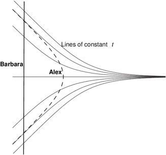
Figure 8: Alex’s hypersurfaces of simultaneity as described in Barbara’s $(\tau,\rho)$ coordinates, for the ‘Uniformly Accelerating’ case.

The metric in these coordinates is $ds^{2}=e^{2a\rho}(d\tau^{2}-d\rho^{2})$. Although Barbara has a ‘straight trajectory’ in these coordinates, she is still undergoing an acceleration $a$, just as we undergo a constant acceleration g through being ‘held up’ against the earth’s gravitational field. (Of course Barbara is here being ‘pulled down’ rather than pulled ‘towards the earth’s centre’, so no tidal forces are involved.) Although Alex’s trajectory appears curved in these coordinates, he is still inertial, since his trajectory is geodesic in this metric. Alex and Barbara’s proper times are unaltered by this change of coordinates, so that it is still Alex who ages more during his absence from Barbara. Some of the lines of constant $t$, which represent Alex’s hypersurfaces of simultaneity, fail to intercept his trajectory in Figure 8. This is because Barbara’s $(\tau,\rho)$ coordinates cover only region U of Figure 7, so any line of constant $t$ which intercepts Alex’s trajectory in region F or P will not have the interception visible in Figure 8.

A similar coordinate transformation can be performed for the ‘Immediate Turn-around’ case. In $(\tau,\rho)$ coordinates this is shown in Figure 9.

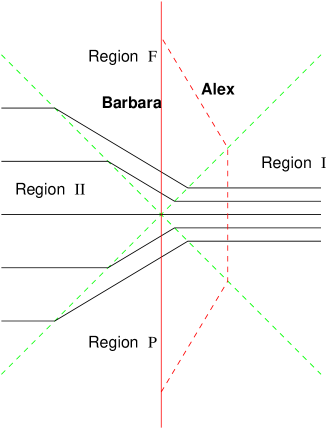
Figure 9: Alex’s hypersurfaces of simultaneity, as described in Barbara’s $(\tau,\rho)$ coordinates, for the ‘Immediate Turn-around’ case.

The metric in these coordinates is:

$$ds^{2}=\begin{cases}e^{-2\alpha}(d\tau^{2}-d\rho^{2})&\mbox{region II}\\ (d\tau^{2}-d\rho^{2})&\mbox{regions F,P}\\ e^{2\alpha}(d\tau^{2}-d\rho^{2})&\mbox{region I}\\ \end{cases}$$

which is Minkowski in all 4 regions, but with a shock-like scale discontinuity along the lines $x=\pm t$ which causes geodesics to ‘turn left’ upon crossing these lines. In these coordinates Alex’s hypersurfaces of simultaneity look much as Barbara’s did in the original coordinate system. It is still Alex who is inertial, however. Graphing the results in different coordinate systems makes no difference to this conclusion. Also, since the definition of radar time is independent of the choice of coordinates, then any statement that Barbara makes of the form ‘Alex did this at this time’ (according to her), or any statement that Alex makes of the form ‘Barbara did this at this time’ (according to him), will be unchanged by changes in coordinates.

CONCLUSION

We have demonstrated that ‘radar time’ is applicable to arbitrarily moving observers, and we have used it to find the hypersurfaces of simultaneity of the travelling twin in the ‘twin paradox’. Radar time allows the travelling twin to assign times to distant events in a fully coordinate invariant fashion. We have considered a general class of twins, varying from the ‘Immediate Turn-around’ case to the ‘Uniformly Accelerating’ observer, and have highlighted some common misconceptions.

Throughout this paper we have made a convenient but unrealistic simplification. It is clear from the trajectories shown in the previous figures that Barbara and Alex could not possibly be twins, since they never spend more than an instant in each other’s company. More realistically, Barbara’s trajectory should coincide with Alex’s until she begins her journey, and should coincide again after her return. The hypersurfaces of simultaneity for this more realistic trajectory are shown in Figure 10.

Figure 10: Hypersurfaces of simultaneity of the travelling twin in the more realistic case, in which their trajectories coincide before and after the journey.

In the causal envelope${}^{\mbox{\scriptsize\cite[cite]{[\@@bibref{}{Pauri}{}{}]}}}$ of Barbara’s journey (that is: the intersection of the causal future of her departure and the causal past of her return, being the middle four regions in Figure 10) these hypersurfaces are identical to those of Figure 5. Readers might enjoy interpreting the rest of this diagram, convincing themselves that the length of the left arrow represents Barbara’s travelling time and that the length of the middle arrow represents Alex’s, and verifying that the ratio of these is indeed $\sqrt{1-s^{2}}$.

References

- [1] D. Bohm, The Special Theory of Relativity (W. A. Benjamin, 1965).
- [2] R. D’Inverno, Introducing Einstein’s Relativity (Oxford University Press, 1992).
- [3] L. Sartori, Understanding Relativity: a simplified approach to Einstein’s theories (University of California Press, 1996).
- [4] W. Pauli, Theory of Relativity (Pergamon Press, 1958).
- [5] W. G. Unruh, “Parallax distance, time, and the twin ‘paradox’,” Am. J. Phys. 49(6), 589–592 (1981).
- [6] T. A. Debs & M. L. G. Redhead, “The twin ‘paradox’ and the conventionality of simultaneity”, Am. J. Phys. 64(4) 384–392 (1995).
- [7] L. Marder, Time and the Space-Traveller (George Allen & Unwin Ltd., 1971).
- [8] C. W. Misner, K. S. Thorne & J. A. Wheeler, Gravitation (W. H. Freeman & Co., 1973).
- [9] A. Einstein, “On the Electrodynamics of Moving Bodies,” Annalen der Physik 17, 891–921 (1905).
- [10] M. Pauri & M. Vallisneri, “Märzke-Wheeler Coordinates for Accelerated Observers in Special Relativity,” Found. Phys. Lett. 13(5) 401–425 (2000).
- [11] H. Bondi, Assumption and Myth in Physical Theory (Cambridge University Press, 1967).
- [12] P. C. W. Davies, About Time (Orion Productions, 1995).