Functional Schrödinger Picture for Conformally Flat Space-Time with Cosmological Constant

Abstract

A quantum-field model of the conformally flat space is formulated using a standard field-theoretical technique, a probability interpretation and a way to establish the classical limit. The starting point is the following: after conformal transformation of the Einstein – Hilbert action, the conformal factor represents a scalar field with the negative kinetical term and the self-interaction inspired by the cosmological constant. (It has been found that quanta of such action have a negative value as a sequence of the negative energy.) The metric energy-momentum tensor of this scalar field is proportional to the Einstein tensor for the initial metric. Therefore, a vacuum state of the field is treated as a classical space. In such vacuum the zero mode is a scale factor of the flat Friedmann Universe. It is shown that conformal factor may be viewed as a an inflaton field, and its small non-homogeneities represent gauge invariant scalar metric perturbations.

PACS number: 98.80.Hw Quantum Cosmology

I Introduction

The metric of the conformally flat space-time only contains one essential variable – a conformal factor [1] which is a scale factor of the expanding Universe. The negative energy of this variable leads to the difficulties in the quantum cosmology based on the Wheeler – DeWitt equation  [2] (for example, the wave function of the Universe is non-normalazible, a probability current density is not positive definite). Different ways are used to overcome these obstacles. Matter or scale factor sometimes are treated as non-dynamical. Neglecting an interaction between matter and scale factor allows one to factorize the wave function and to include a minus sign into the time or the energy in the stationary Schrödinger equation for scale factor. For example, Narlikar and Padmanabhan [6] introduce stationary states of the quantum geometry as a solution of such an equation to prevent classical singularity. However, in this approach the conformal factor is treated as a physical variable while its energy is considered as an unphysical one. Hence it seems rather strange that this energy may compensate the energy of the created matter [5]. Another interesting result of the quantization of the conformal factor via Feynman path integral derived by these authors is the growing of the quantum fluctuations near the singularity [6]. But the Euclidian path integral for gravity is divergent because the Euclidian gravitational action is not positive-definite [7]. Gravitational waves carry positive energy and gravitational potential energy is negative. Conformal rotation (using the complex conformal factor [8]) makes an Euclidian path integral convergent by changing the sign of the action . But this method is applicable only if the conformal factor is an unphysical variable (as in asymptotically flat space-time) [9] .

In Friedmann – Robertson – Walker Universe, the conformal factor is a single degree of freedom [2]. It must be a physical variable because the expansion of the Universe is an observational fact .

To conclude the brief review of theoretical works dealing with quantization of the conformal factor, one can say that there is no completely satisfying quantum picture of the expansion of the Universe. The main questions are gravitational degrees of freedom and gravitational energy.

Experimental data point out an accelerating expansion of the Universe, and hence, the cosmological constant may carry a significant contribution into the energy density [15]. It is a difficult question to the quantum field theory why the expected vacuum energy density is much greater than that corresponding to the cosmological constant [16]. Inflation theories exploit a state equation related to the cosmological constant but they do not explain the mentioned contradiction [17, 18]. Meanwhile, the large scale structure of the Universe and the cosmic background radiation anisotropy are treated as consequences of quantum fluctuation of inflaton field [19] or quantum metric fluctuation [20] . A modern tool for studying the inflation is a non-equilibrium phase transition dynamics [22] in the field theoretical Schrödinger picture [23].

So the quantum model of the conformally flat space-time looks interesting from a theoretical viewpoint and may link quantum cosmology to the observational data.

In this paper, attempt is made to quantize the conformally flat space-time in the Schrödinger picture by a standard field theoretical technique. Two main circumstances are taken into account. First, the geometrical and field properties of the space-time are split in the Einstein – Hilbert action via a conformal transformation. The equation of motion for the gravitational field (conformal factor) is derived by variation of the action with respect to a field variable and represents a Klein – Gordon equation with additional Penrous – Chernicov – Tagirov term [24]. The metric energy-momentum tensor [24] of the field is derived by variation of the action with respect to new metric (Minkowcki metric for conformally flat space-time discussed here) and is proportional to Einstein equations for the initial metric. Thus a vacuum state of the field (where the energy-momentum tensor overage is zero) is considered as a classical space-time. Second, it is taken into account that a system with negative energy needs to be quantized using Planck constant with a negative sign according to the Bohr – Sommerfeld rule and to analogy between wave mechanic and geometric optics.

The paper is organized as follows. Section II represents the conformally flat space-time with the cosmological constant as a self-interacting scalar field in Minkowski space-time. In Section III quantization of the oscillating modes is fulfilled while zero mode is considered as a classical quantity. Section IV gives a relation of the conformal factor to an inflaton field and to scalar metric perturbations. The Summary reviews the construction of the model, discusses main results, and compares with some related works. Quantization of the system with the negative energy (inverted harmonic oscillator) is prepared in Appendix A. Some used formulae for Bessel functions are given in Appendix B.

II Representation of the conformally flat space-time by a scalar field

To describe the conformally flat Universe by a scalar field in Minkowski space-time, we use conformally flat coordinates. Let us suppose that there is a general coordinate transformation

$$x=x(\tilde{x}),\;\;g_{ij}(x)=\frac{\partial\tilde{x}^{l}}{\partial x^{i}}\frac{\partial\tilde{x}^{m}}{\partial x^{j}}\tilde{g}_{lm}(\tilde{x}),\;\;\;\;i,j=1,2,3,4$$ (1)

$$ds^{2}=g_{ij}(x)dx^{i}dx^{j}=\tilde{g}_{ij}(\tilde{x})d{\tilde{x}}^{i}d{\tilde{x}}^{j},$$ (2)

after which the new metric has a common multiplier (conformal factor):

$$\tilde{g}_{ij}(\tilde{x})=a^{2}(\tilde{x}){g^{\prime}}_{ij}(\tilde{x}),$$ (3)

$$ds^{2}=a^{2}(\tilde{x})(ds^{\prime})^{2},\;\;\;\;(ds^{\prime})^{2}={g^{\prime}}_{ij}(\tilde{x})d\tilde{x}^{i}d\tilde{x}^{j}.$$ (4)

The equations for metric $\tilde{g}_{ij}(\tilde{x})$ following from Einstein – Hilbert action

$$S[\tilde{g}(\tilde{x})]=-\int\limits d^{4}\tilde{x}\sqrt{-\tilde{g}}\left(\tilde{R}+\Lambda\right),\;\;\;\;\Lambda>0,$$ (5)

can be written as equations for conformal factor $a(\tilde{x})$ and metric ${g^{\prime}}_{ij}(\tilde{x})$

$$\tilde{G}_{ij} = \tilde{R}_{ij}(\tilde{x})-\frac{1}{2}\tilde{R}(\tilde{x})\tilde{g}_{ij}(\tilde{x})-\Lambda\tilde{g}_{ij}(\tilde{x})$$ (6)

$$= {R^{\prime}}_{ij}(\tilde{x})-\frac{1}{2}R^{\prime}(\tilde{x}){g^{\prime}}_{ij}(\tilde{x})$$ (9)

$$+a^{-2}(\tilde{x})[-\nabla_{i}\nabla_{j}a^{2}(\tilde{x})+6\partial_{i}a(\tilde{x})\partial_{j}a(\tilde{x})$$

$$+{g^{\prime}}_{ij}(\tilde{x})(\Box a^{2}(\tilde{x})-3\partial^{n}a(\tilde{x})\partial_{n}a(\tilde{x})-\Lambda a^{4}(\tilde{x}))].$$

From the other hand, the Einstein – Hilbert action (5) can be rewritten by using the conformal transformation formulae [27] corresponding to factorization of the metric (3)

$$\tilde{R}(\tilde{x})=a^{-2}\left(R^{\prime}(\tilde{x})-6a^{-1}(\tilde{x})\Box a(\tilde{x})\right),\;\;\;\mbox{ }\;\;\;\Box a(\tilde{x})=\frac{1}{\sqrt{-g^{\prime}}}\partial_{i}\left(\sqrt{-g^{\prime}}(g^{\prime})^{ij}\partial_{j}a\right)$$ (10)

$$\sqrt{-\tilde{g}(\tilde{x})}=a^{4}(\tilde{x})\sqrt{-g^{\prime}(\tilde{x})}.$$ (11)

As a result, an action for a scalar field $a(\tilde{x})$ with negative kinetic term in metric ${g^{\prime}}_{ij}(\tilde{x})$ [7] appears

$$S[g^{\prime}(\tilde{x}),a(\tilde{x})]=-\int\limits d^{4}{\tilde{x}}\sqrt{-g^{\prime}}\left(\frac{1}{2}(g^{\prime})^{ij}\partial_{i}a\partial_{j}a+\frac{1}{12}a^{2}R^{\prime}+\frac{\lambda}{4!}a^{4}\right),$$ (12)

where $\lambda=4\Lambda$. Total divergence and numerical factor are neglected. Variation of this action with respect to metric ${g^{\prime}}_{ij}$ gives a metric energy-momentum tensor [24] of the conformal scalar field $a(\tilde{x})$

$$T^{(metr)}_{ij}=T^{(can)}_{ij}-\frac{1}{6}\left({R^{\prime}}_{ij}+{g^{\prime}}_{ij}\Box-\nabla_{i}\nabla_{j}\right)a^{2},$$ (13)

where the canonical energy-momentum tensor has the form

$$T^{(can)}_{ij}=-\partial_{i}a\partial_{j}a+{g^{\prime}}_{ij}\left(\frac{1}{2}\partial^{n}a\partial_{n}a+\frac{1}{12}a^{2}R^{\prime}+\frac{\lambda}{4!}a^{4}\right).$$ (14)

The metric energy-momentum tensor (13) is proportional to the Einstein equations (6)

$$T^{(metr)}_{ij}=-\frac{a^{2}}{6}\tilde{G}_{ij}.$$ (15)

This fact can be directly deduced if we mention that both quantities are derived by variation of the Einstein – Hilbert action with respect to the metrics which are proportional each other as it follows from (3) . The metric energy-momentum tensor trace is equal to zero on the equation of motion for $a(\tilde{x})$

$$\frac{1}{6}a^{3}\tilde{G}=-a^{-1}T=\Box a-\frac{1}{6}aR^{\prime}-\frac{\lambda}{6}a^{3}.$$ (16)

So this equation of motion expresses a condition for conformal invariance. The interaction that arises due to the cosmological constant is a unique possible conformally invariant one. We see from (15) that the metric energy-momentum tensor (13) must be equal to zero to be consistent with Einstein equations (6). Let us suppose that there is a state in quantum field theory of the conformal factor $a(x)$ with a vanishing averaged value for the energy-momentum tensor

$$\langle 0|T_{ij}|0\rangle=0,\;\;\;\langle 0|0\rangle=1.$$ (17)

Such a state naturally is a vacuum state and corresponds to the classical theory.

In the case of the conformally flat space-time we can consider the transformation (1) as a transformation to the conformally flat coordinates $\tilde{x}$ . Hence, the metric ${g^{\prime}}_{ij}(\tilde{x})$ arising due to factorization of the ${\tilde{g}}_{ij}(\tilde{x})$ (3) is Minkowski one:

$${g^{\prime}}_{ij}(\tilde{x})=\eta_{ij}=(+,-,-,-),$$ (18)

and the curvature depending terms disappear from the action (12) and from the energy-momentum tensor (13)

$$S[a(x)]=-\int\limits d^{4}x\left(\frac{1}{2}\partial^{n}a\partial_{n}a+\frac{\lambda}{4!}a^{4}\right),$$ (19)

$$T_{ij}=-\partial_{i}a\partial_{j}a+\frac{1}{6}\partial_{i}\partial_{j}a^{2}+\eta_{ij}\left(-\frac{1}{6}\Box a^{2}+\frac{1}{2}\partial^{n}a\partial_{n}a+\frac{\lambda}{4!}a^{4}\right).$$ (20)

The energy-momentum tensor (20) differs from the canonical one by second derivative terms. But the corresponding Hamiltonian may be derived in usual form after removing a total divergence.

The solution to the Einstein equations (6) is the de Sitter space-time with the curvature scalar $R=-\lambda$. In coordinates $\tilde{x}$ it looks like the spatially flat Friedmann – Robertson – Walker Universe with a cosmological constant. Isometries of the conformally flat space-time preserve the factorization of the metric $\tilde{g}_{ij}(\tilde{x})$ and action (12). All conformally flat spaces have the same conformal group symmetry  [30]. In particular, de Sitter group generators undergo to Poincaré group ones in the limit of the large curvature radius [31] (small cosmological constant). A correct description of the classical Universe will be guaranteed by a conserved energy-momentum tensor providing that the field $a(x)$ has a non-zero vacuum averaged value $a(\eta)$ (it will be shown that $\eta$ corresponds to conformal time in the classical limit) playing the role of a scale factor for the classical metric

$$a(\eta,x)=a(\eta)+\delta a(\eta,x),$$ (21)

where

$$a(\eta)\gg|\delta a(\eta,x)|.$$ (22)

Vacuum fluctuations will cause increase of $a(\eta)$ due to instability of the system with the action (19).

The result of the analysis is the following. After factorization of the conformal factor, the Einstein – Hilbert action looks like a conformal scalar field action with the negative kinetic term. The Einstein equations for the initial metric  (6) are proportional to the metric energy-momentum tensor of the field (13). Hence, the classical conformally flat space-time can be represented as a vacuum state of the unstable scalar field in Minkowski space-time. The energy-momentum tensor vacuum average must be zero and the vacuum field average is a classical scale factor.

III Field-theoretical Schrödinger picture

The most suitable approach to quantization of the model (19), (20) is the Schrödinger picture which has advantages in time-dependent problems [23]. The aim of the quatization is to find a ground state of the system and to construct creation and annihilation operators. This is done in the way proposed Guth and Pi [32] where the inflaton field with self-interaction $\lambda\phi^{4}$ was quantized (in the de Sitter metric) to study the “slow-rollover” phase transition in the new inflation model. Here the problem has been formulated in Minkowski metric but due to instability of the system, the field zero mode dynamics leads to an effect appearing in the non-stationary metric. The field $a(x)$ is decomposed into the Fourier series

$$a(\eta,x)=\sqrt{2}a_{o}(\eta)+\sum_{\vec{k}}[a^{+}_{\vec{k}}(\eta)\cos\vec{k}\cdot\vec{x}+a^{-}_{\vec{k}}(\eta)\sin\vec{k}\cdot\vec{x}],$$ (23)

in a cub with a side $b=2\pi$ using real functions with the following properties

$$a^{+}_{-\vec{k}}(\eta)\equiv a^{+}_{\vec{k}}(\eta),\;\;\;\;a^{-}_{-\vec{k}}(\eta)\equiv-a^{-}_{\vec{k}}(\eta).$$ (24)

The approximation

$$a_{o}(\eta)\gg a^{\pm}_{\vec{k}}(\eta)$$ (25)

corresponds to the classical limit condition (22). Further simplification is to neglect the interaction between the modes $a^{\pm}_{\vec{k}}(\eta)$ in virtue of a small value of $\lambda$. Then the action (19) takes the form

$$S=\int\limits d\eta\left\{-\dot{a}^{2}_{o}(\eta)-\frac{\lambda}{3!}a^{4}_{o}(\eta)+\sum_{k}\left[-\dot{a}^{2}_{k}(\eta)+(k^{2}-\lambda a^{2}_{o}(\eta))a^{2}_{k}(\eta)\right]\right\},$$ (26)

where only one sign modes are presented, their notation is simplified and a space integration is prepared.

A Solution of a classical problem

The action (26) leads to equations of motions

$$\left\{\begin{array}[]{l}\ddot{a}_{o}(\eta)-\frac{\lambda}{3}a^{3}_{o}(\eta)-\lambda a_{o}(\eta)\sum_{k}a^{2}_{k}(\eta)=0,\\ \\ \ddot{a}_{k}(\eta)+(k^{2}-\lambda a_{o}^{2}(\eta))a_{k}(\eta)=0,\end{array}\right.$$ (27)

which self-consistently describe independent oscillators $a_{k}(\eta)$ in external field $a_{o}(\eta)$. Not self-consistent analitically solvable problem does not take into account the $a_{k}(\eta)$-modes influence on zero mode

$$\left\{\begin{array}[]{l}\ddot{a}_{o}(\eta)-\frac{\lambda}{3}a^{3}_{o}(\eta)=0,\\ \\ \ddot{a}_{k}(\eta)+(k^{2}-\lambda a_{o}^{2}(\eta))a_{k}(\eta)=0.\end{array}\right.$$ (28)

The first integral for a zero mode equation

$$\dot{a}_{o}^{2}(\eta)-\frac{\lambda}{6}a^{4}_{o}(\eta)=0.$$ (29)

must be equal to zero according to the correspondence condition (15). The second integration constant can be fixed by assumption that the origin of the time $\eta$ (the conformal time for the Friedmann – Robertson – Walker interval [26]) coincides with the origin of the proper time in synchronous coordinate system

$$dt_{pr}=\sqrt{2}a_{o}(\eta)d\eta.$$ (30)

So $a_{o}(\eta)$ is a scale factor of the flat Friedmann Universe with the cosmological constant

$$a_{o}=\frac{\sqrt{6/\lambda}}{1-\eta}=\sqrt{\frac{6}{\lambda}}\exp\left\{\sqrt{\frac{\lambda}{12}}t_{pr}\right\}$$ (31)

considered in the intervals

$$\begin{array}[]{rcl}0\leq&\eta&<1\\ 0\leq&t_{pr}&<\infty\\ \sqrt{\frac{6}{\lambda}}\leq&a_{o}&<\infty.\\ \end{array}$$ (32)

The equation for oscillating modes $a_{k}(\eta)$ (28) can be reduced to the equation for Bessel functions

$$\frac{d^{2}\xi(\tau_{k})}{d\tau^{2}_{k}}+\frac{1}{\tau_{k}}\frac{d\xi(\tau_{k})}{d\tau_{k}}+\left(1-\frac{\nu^{2}}{\tau^{2}_{k}}\right)\xi(\tau_{k})=0$$ (33)

with the index $\nu=5/2$ by change of variables

$$\tau_{k}=k(1-\eta),\;\;a_{k}(\tau_{k})=\xi(\tau_{k})\sqrt{\tau_{k}}.$$ (34)

The general solution for $a_{k}(\eta)$ is a linear combination

$$a_{k}(\eta)=\frac{1}{\sqrt{2}}\left[A_{k}\psi_{k}(\eta)+A^{\dagger}_{k}\psi^{*}_{k}(\eta)\right],$$ (35)

where $A_{k},A^{\dagger}_{k}$ are coefficients, and $\psi_{k}(\eta),\psi^{*}_{k}(\eta)$ are expressed in terms of Hankel functions

$$\psi_{k}(\eta)=\frac{1}{2}\sqrt{\pi\hbar(1-\eta)}H^{(1)}_{\frac{5}{2}}\Bigl{(}k(1-\eta)\Bigr{)},\;\;\psi^{*}_{k}(\eta)=\frac{1}{2}\sqrt{\pi\hbar(1-\eta)}H^{(2)}_{\frac{5}{2}}\Bigl{(}k(1-\eta)\Bigr{)}.$$ (36)

Functions $\psi_{k}(\eta),\psi^{*}_{k}(\eta)$ satisfy the orthogonality condition

$$\psi_{k}(\eta)\frac{\partial}{\partial\eta}\psi^{*}_{k}(\eta)-\psi^{*}_{k}(\eta)\frac{\partial}{\partial\eta}\psi_{k}(\eta)=i\hbar.$$ (37)

Using this relation, the coefficients $A_{k},A^{\dagger}_{k}$ can be written as follows:

$$A_{k}=\frac{\sqrt{2}}{i\hbar}\left(a_{k}(\eta)\frac{\partial}{\partial\eta}\psi^{*}_{k}(\eta)-\psi^{*}_{k}(\eta)\frac{\partial}{\partial\eta}a_{k}(\eta)\right),\;\;\;A^{\dagger}_{k}=-\frac{\sqrt{2}}{i\hbar}\left(a_{k}(\eta)\frac{\partial}{\partial\eta}\psi_{k}(\eta)-\psi_{k}(\eta)\frac{\partial}{\partial\eta}a_{k}(\eta)\right).$$ (38)

The equality

$$A^{*}_{k}=A^{\dagger}_{k}$$ (39)

holds as the field $a(\eta,x)$ has a real value.

B Quantization of oscillatory modes

As zero mode $a_{o}(\eta)$ is a classical quantity in the accepted approximation (25), only oscillating modes $a_{k}(\eta)$ must be quantized as independent variables. Due to the negative kinetic energy, the conjugated momentum has an opposite sign with respect to time derivative of the $a_{k}(\eta)$

$$\pi_{k}(\eta)=\frac{\partial L}{\partial\dot{a}_{k}(\eta)}=-2\dot{a}_{k}(\eta).$$ (40)

The momentum operator is as follows (see Appendix A)

$$\pi_{k}\;\to\;i\hbar\frac{\delta}{\delta a_{k}}.$$ (41)

The commutator also differs from that in a usual case by sign

$$[a_{k},\pi_{k^{\prime}}]=-i\hbar\delta_{kk^{\prime}}.$$ (42)

The wave functional of the system is a product of the mode functionals in the case of the absence of interactions

$$\Psi=\prod_{k}\Psi_{k}(\eta),\;\;\;\;\Psi_{k}(t)\equiv\Psi_{k}[a_{k},\eta].$$ (43)

The Schrödinger equation for $\Psi_{k}(\eta)$

$$-i\hbar\frac{\partial}{\partial\eta}\Psi_{k}(\eta)=H_{k}\Psi_{k}(\eta)$$ (44)

with the Hamiltonian

$$H_{k}=-\frac{\pi^{2}_{k}}{4}-(k^{2}-\lambda a^{2}_{o}(\eta))a^{2}_{k},$$ (45)

where $a_{o}(\eta)$ is a known function (31), can be solved by usual ansatz [32]

$$\Psi_{k}(\eta)=C_{k}(\eta)\exp\left\{-2\Omega_{k}(\eta)a^{2}_{k}\right\},$$ (46)

where a covariance $\Omega_{k}(\eta)$ is introduced

$$\Omega_{k}(\eta)=-\frac{i}{2\hbar}\frac{\dot{\varphi}^{*}_{k}(\eta)}{\varphi^{*}_{k}(\eta)}.$$ (47)

The equations for $C_{k}(\eta)$ and $\varphi^{*}_{k}(\eta)$ follow from the Schrödinger equation (44)

$$\left\{\begin{array}[]{l}\frac{\dot{C}_{k}(\eta)}{C_{k}(\eta)}=-\frac{1}{2}\frac{\dot{\varphi}^{*}_{k}(\eta)}{\varphi^{*}_{k}(\eta)},\\ \\ \ddot{\varphi}^{*}_{k}(\eta)+(k^{2}-\frac{6}{(1-\eta)^{2}})\varphi^{*}_{k}(\eta)=0.\end{array}\right.$$ (48)

The solution for $\varphi_{k}(\eta)$ is analogous to this for $\psi_{k}(\eta)$ (36)

$$\varphi_{k}(\eta)=\frac{1}{2}\sqrt{\pi\hbar(1-\eta)}\left(c_{1}H^{(1)}_{\frac{5}{2}}\Bigl{(}k(1-\eta)\Bigr{)}+c_{2}H^{(2)}_{\frac{5}{2}}\Bigl{(}k(1-\eta)\Bigr{)}\right)$$ (49)

with the same normalization (37) suggesting a condition

$$|c_{1}|^{2}-|c_{2}|^{2}=1.$$ (50)

The coefficient $C_{k}(\eta)$ in the wave functional (46) can be expressed via function $\varphi_{k}(\eta)$

$$\Bigl{|}C_{k}(\eta)\Bigr{|}=\left(\pi|\varphi_{k}|^{2}\right)^{-1/4}$$ (51)

according to (48) and to normalization condition

$$\int\limits{\cal D}a_{k}\Psi^{*}_{k}(t)\Psi_{k}(t)=1.$$ (52)

The real and imaginary parts of the covariance $\Omega_{k}(\eta)$ are as follows

$$Re\,\Omega_{k}(\eta)=\frac{1}{4|\varphi_{k}|^{2}},\;\;\;Im\,\Omega_{k}(\eta)=-\frac{1}{4\hbar|\varphi_{k}|^{2}}\frac{\partial}{\partial\eta}|\varphi_{k}|^{2}.$$ (53)

Hence, the functional $\Psi_{k}(\eta)$ (46) is determined. It corresponds to the Bunch – Davies vacuum [33] of the scalar field in the de Sitter space which is a unique, completely de Sitter invariant vacuum state [32]. As it was stressed in [34] , owing to conformal invariance, the situation is as in flat space-time, where a unique Poincaré invariant vacuum exists.

We demand $A_{k}$ (38) to be an annihilation operator

$$A_{k}\Psi_{k}(\eta)=0.$$ (54)

This equality is satisfied by choosing $c_{1}\!=\!1$ in solution $\varphi_{k}(\eta)$ (49), hence we have $\varphi_{k}(\eta)\equiv\psi_{k}(\eta)$ ($c_{2}=0$ from (50)). The annihilation $A_{k}$ and creation $A^{\dagger}_{k}$ operators (38) are the following:

$$A_{k}=\frac{\psi^{*}_{k}(\eta)}{\sqrt{2}}\left(4\Omega_{k}(\eta)a_{k}-\frac{i}{\hbar}\pi_{k}\right),\;\;\;A^{\dagger}_{k}=\frac{\psi_{k}(\eta)}{\sqrt{2}}\left(4\Omega^{*}_{k}(\eta)a_{k}+\frac{i}{\hbar}\pi_{k}\right).$$ (55)

They satisfy the usual commutation relation

$$[A_{k},A^{\dagger}_{k^{\prime}}]=\delta_{kk^{\prime}}$$ (56)

which preserves a positive definitized norm of the state functional.

Using expressions for operators $a_{k},\pi_{k}$ via operators $A_{k},A^{\dagger}_{k}$ (55)

$$a_{k}=\frac{1}{\sqrt{2}}(\psi_{k}(\eta)A_{k}+\psi^{*}_{k}(t)A^{\dagger}_{k^{\prime}}),$$ (57)

$$\pi_{k}=i\hbar 2\sqrt{2}(\psi_{k}(\eta)\Omega^{*}_{k}(\eta)A_{k}-\psi^{*}_{k}(\eta)\Omega_{k}(t)A^{\dagger}_{k})=-\sqrt{2}(\dot{\psi}_{k}(\eta)A_{k}+\dot{\psi}^{*}_{k}(\eta)A^{\dagger}_{k}),$$ (58)

we can rewrite the Hamiltonian (45) in terms of creation and annihilation operators

$$H = -\frac{1}{2}\left\{A_{k}A_{k}\left(\dot{\psi}^{2}_{k}(\eta)+(k^{2}-\frac{6}{(1-t)^{2}})\psi^{2}_{k}(\eta)\right)\right.$$ (61)

$$+(A^{\dagger}_{k}A_{k}+A_{k}A^{\dagger}_{k})\left(\dot{\psi}_{k}(\eta)\dot{\psi}^{*}_{k}(\eta)+(k^{2}-\frac{6}{(1-\eta)^{2}})\psi_{k}(\eta)\psi^{*}_{k}(\eta)\right)$$

$$\left.+A^{\dagger}_{k}A^{\dagger}_{k}\left((\dot{\psi}^{*}_{k}(\eta))^{2}+(k^{2}-\frac{6}{(1-\eta)^{2}})(\psi^{*}_{k}(\eta))^{2}\right)\right\}.$$

As functions $\psi_{k}(\eta)$ tend to oscillator functions when $t\to 0$, this Hamiltonian tends to the oscillator Hamiltonian for large $k$.

It is interesting to find a time dependence for the vacuum fluctuations and for the one-particle excitation energy. Fluctuations are determined by real part of the covariance $\Omega_{k}(\eta)$ (53)

$$\langle a^{2}_{k}\rangle=\int\limits{\cal D}a_{k}\Psi^{*}_{k}(\eta)a^{2}_{k}\Psi_{k}(\eta)=\frac{1}{2}|\varphi_{k}|^{2}=\frac{1}{8Re\,\Omega_{k}(\eta)}.$$ (62)

The one-particle state

$$\Psi_{1k}(\eta)=A^{\dagger}_{k}\Psi_{k}(\eta)=\sqrt{2}\frac{\psi_{k}(\eta)}{|\psi_{k}|^{2}}a_{k}\Psi_{k}(\eta),\;\;\;\langle\Psi^{*}_{1k}(\eta)|\Psi_{1k}(\eta)\rangle=1$$ (63)

has the energy

$$E_{1k}=\langle\Psi^{*}_{1k}(\eta)|H_{k}|\Psi_{1k}(\eta)\rangle-\langle\Psi^{*}_{k}(\eta)|H_{k}|\Psi_{k}(\eta)\rangle=-\dot{\psi}_{k}(\eta)\dot{\psi}^{*}_{k}(\eta)-\psi_{k}(\eta)\psi^{*}_{k}(\eta)\left(k^{2}-\frac{6}{(1-\eta)^{2}}\right),$$ (64)

where the vacuum energy is subtracted. The potential part of the energy shows that the oscillations of the mode with the wave number $k\!>\!\sqrt{6}$ break down at the moment $\eta=T_{k}$

$$T_{k}=1-\frac{\sqrt{6}}{k}.$$ (65)

At this moment the potential becomes non-oscillatory, the amplitude and fluctuations of the mode begin to grow. Explicit time dependence of the energy is the following

$$E_{1k}=-\frac{\hbar k}{2}\zeta^{-6}(2\zeta^{6}-6\zeta^{4}-9\zeta^{2}-18),\;\;\;\zeta=k(1-\eta),$$ (66)

where an analytic expression for the spherical Bessel function is used (see Appendix B). For small $\eta\ll 1$ and large $k\gg\sqrt{6}$ (that means $\zeta\gg 1$) the excitation energy is like a negative oscillator energy $E=-\hbar k$. As the time grows ($\eta\!\to\!1$), the lower bound for oscillating modes wave number $k$ rises. After time $\eta=T_{k}$ (65) a moment comes when the excitation energy changes the sign. It can be seen from expression for $E_{1k}$ (66) in the limit $\zeta\ll 1$ ($\eta\!\approx\!1$).

IV Relation of the conformal factor to an inflaton field and to cosmological perturbations

In this section two issues are discussed. The former is to show how to present conformal factor as an inflaton field. The latter shows how fluctuations of the conformal factor are included into the theory of the cosmological perturbations.

As it follows from (62), (49), vacuum fluctuations of the field $a(x)$ are similar to those of the scalar field in the de Sitter metric [32]. To show an equivalence of their dynamical properties explicitly, let us rewrite the equation for $a_{k}$ (28) in proper time (30), simultaneously preparing a conformal transformation [24] of the mode

$$a_{k}=a_{o}\phi_{k}.$$ (67)

The resulting equation is the same as one for a scalar field [32]

$$\frac{d^{2}\phi_{k}}{dt^{2}_{pr}}+3H\frac{d\phi_{k}}{dt_{pr}}+H^{2}\left(k^{2}e^{-2Ht_{pr}}-4\right)\phi_{k}=0,$$ (68)

where $H$ is the Hubble parameter following from solution for $a_{o}$ (31)

$$H=\frac{1}{a_{o}}\frac{da_{o}}{dt_{pr}}=\sqrt{\frac{\lambda}{12}}.$$ (69)

Induced by zero mode mass term $\mu^{2}=4H^{2}$ fixes the Bessel functions index $\nu=5/2$ in according with the result [32] (formula (3.18)). Moreover, the solution for the zero mode of the scalar field (formula (7.6) in [32]) coincides with the solution for $a_{o}$ (31).

Let us show that small non-homogeneities of the conformal factor correspond to those of the two independent gauge invariant functions, which represent cosmological scalar metric perturbations [36]. For spatially flat Robertson – Walker metric, scalar perturbations are represented by two 3-scalar functions $\Phi(\eta,x)$ and $\Psi(\eta,x)$ ($\Phi,\Psi\ll 1$)

$$ds^{2}=a^{2}(\eta)\left[(1+2\Phi(\eta,x))d\eta^{2}-(1-2\Psi(\eta,x))\delta_{\alpha\beta}dx^{\alpha}dx^{\beta}\right].$$ (70)

In terms of new variables

$$C(\eta,x)=\frac{1}{2}\left(\Phi(\eta,x)-\Psi(\eta,x)\right),\;\;\;\;N(\eta,x)=\frac{1}{2}\left(\Phi(\eta,x)+\Psi(\eta,x)\right)$$ (71)

the perturbed interval looks like

$$ds^{2}=a^{2}(\eta)(1+2C(\eta,x))\left[(1+2N(\eta,x))d\eta^{2}-(1-2N(\eta,x))\delta_{\alpha\beta}dx^{\alpha}dx^{\beta}\right].$$ (72)

Function $C(\eta,x)$ represents conformal factor fluctuations, and function $N(\eta,x)$ is a generalization of the Newtonian potential. The trace of the equations for the cosmological perturbations without matter is as follows ($N(\eta,x)\equiv 0$)

$$\ddot{C}+2{\cal H}\dot{C}-\nabla^{2}C-2({\cal H}^{2}+\dot{\cal H})C=0$$ (73)

where $\dot{C}\equiv{dC}/{d\eta},\;{\cal H}=\frac{1}{a}\frac{da}{d\eta}$, $\nabla^{2}$ is Laplacian in the space metric $\delta_{\alpha\beta}$. A relation between function $C(\eta,x)$ and conformal factor $a(\eta,x)$ follows from comparison of the form of the intervals (72) and (2). The latter is following in the present paper

$$ds^{2}=a^{2}(\eta,x)[d\eta^{2}-\delta_{\alpha\beta}dx^{\alpha}dx^{\beta}].$$ (74)

Taking into account decomposition (23) of the conformal factor $a(\eta,x)$, one can deduce

$$C(\eta,x)\approx\frac{1}{\sqrt{2}a_{o}(\eta)}\sum_{\vec{k}}[a^{+}_{\vec{k}}(\eta)\cos\vec{k}\cdot\vec{x}+a^{-}_{\vec{k}}(\eta)\sin\vec{k}\cdot\vec{x}],\;\;\;\;a(\eta)=\sqrt{2}a_{o}(\eta)$$ (75)

where $a_{o}(\eta)$ is considered as a known function (31). Then eq. (73) for the function $C(\eta,x)$ completely coincides with the eq. (27) for modes $a_{k}(\eta)$

$$\ddot{a}_{k}+(k^{2}-\lambda a_{o}^{2})a_{k}=0.$$ (76)

This correspondence follows from the fact that the equation of motion for the conformal factor is proportional to the trace of the Einstein equations according to (16).

So we have showed that the conformal factor (4-scalar) represents a kind of the inflaton field and how it is connected to gauge invariant scalar metric perturbations.

V Summary

The main aim of this work is to get a consistent way to present gravitation as a field living on the flat background and to apply quantum field technique with the well known interpretation (especially, a link between quantum and classical theories) to cosmology. It seems preferable to describe the expansion of the Universe in the functional Schrödinger picture which is suitable for non-stationary processes like a phase transition. Here the problem is solved in the not self-consistent case.

The representation of the conformally flat space-time with the cosmological constant as a self-interacting scalar field in Minkowski world is based on the fact that only one essential metric variable (a conformal factor) describes the investigated model due to the conformal symmetry . After extraction of the conformal factor from the metric, the Einstein – Hilbert action looks like an action for the conformal scalar field with a negative kinetic term and a selfi-nteraction inspired by a cosmological constant. The metric energy-momentum tensor for such a field is proportional to the initial Einstein equations . Hence, a vacuum state (in which energy-momentum tensor average vanishes) corresponds to classical space-time, and the field average is a scale factor of the Universe. From other side, mentioned condition provides a link to the Wheeler – DeWitt approach.

A role of the negative energy in quantum theory is investigated here. In this case the momentum and the velocity of the particle are contrarily directed. If an action is considered as a wave phase, then the constant phase wave will move against a momentum direction. Hence, a coefficient between the momentum and the wave vector must be negative. Further, the negative energy leads to the negative “action”-variable in the Hamilton – Jacobi theory. And the quantum of this “action” must be negative, too. Meanwhile, the minus sign before the Planck constant does not disturb the Dirac’s prescription for the quantization of a classical system. The changing in sign with respect to usual case occurs, for example, in commutator, in momentum operator, in quasi-classical wave function and in the left hand side of the Schrödinger equation. Quantization of the system with the negative energy includes standard steps and a probability interpretation if one follows the procedure suggested here (see appendix A) .

In frames of the suggested model, the classical Universe arises at a stage of the non-stable quantum system evolution when zero mode of the conformal factor becomes much greater then oscillating modes. So the classical space is the vacuum state of this system. The large field vacuum average (zero mode) plays the role of the metric scale factor. Integral of motion for zero mode is the energy vacuum average and must be put to zero to coincide with the corresponding Einstein equation. In result we derive the correct description of the classical Universe. The existence of the field vacuum average is a sequence of the instability of the system (the kinetic energy is negative and self-interaction energy depending of the cosmological constant is positive).

The “phantom” field Lagrangian [44, 45] has negative kinetic and positive potential parts, too . In contrast with the conformal factor, this field is introduced only for getting a negative pressure to explain the accelerating Universe expansion.

The mentioned above peculiarities distinguish the suggested model from Thirring model [47] describing gravity by a scalar field in the field theoretical formulation of the General Relativity in a flat space . In this kind of theories the Universe expansion can not be described because the positive definite Hamiltonian is postulated and small deviations from Minkowski space are supposed [47].

In the model introduced here, the quantum fluctuations are similar to those in the inflation theories [32] because the equations of motion for oscillating modes are the same in both theories. The index of Bessel functions in the solution for the conformal factor is fixed, because the “mass” parameter is connected with the cosmological constant which simultaneously determines the Hubble parameter.

Further it seems interesting to do the following. In the self-consistent case (27), renormalization group running of the interaction constant $\lambda$ can be studied. It must be shown at non-zero temperature that there is a phase transition causing the emergence of the vacuum field average due to quantum fluctuations. Next, the quantum properties of the open, flat and closed Universes can be compared using the fact that the background metric curvature scalar is presented in the conformal field action (12). A possible generalization for an arbitrary metric can be investigated. The most intriguing problem is to incorporate a matter into the model.

A Systems with negative energy

In this Appendix the quantization of a system with the negative energy is discussed on the example of an inverted harmonic oscillator. It is shown that the negative energy causes the minus in front of Planck constant. However we do not need to change the known quantization algorithm and interpretation of a resulting quantum theory.

First of all, let us discuss a difference between a classical motion of a positive particle (with the positive kinetic energy) and of a negative particle (with the negative kinetic energy). We describe them by $L_{+}$ and $L_{-}$ Lagrangians respectively with the same linear potential

$$L_{+}=\frac{m\dot{x}^{2}_{+}}{2}-kx_{+},\;\;\;L_{-}=-\frac{m\dot{x}^{2}_{-}}{2}-kx_{-},\;\;\;\dot{x}_{\pm}=\frac{dx_{\pm}}{dt},$$ (A.1)

where $m\!>\!0,\;\;k\!>\!0$. Their accelerations and velocities are contradictory to each other

$$\ddot{x}_{-}=-\ddot{x}_{+}=\frac{k}{m},\;\;\;\dot{x}_{-}=-\dot{x}_{+}=\frac{k}{m}t.$$ (A.2)

The positive particle moves towards decreasing the potential and the negative particle moves towards increasing the potential

$$x_{-}=-x_{+}=\frac{k}{m}\frac{t^{2}}{2}.$$ (A.3)

From the energy expressions

$$E_{+}=\frac{m\dot{x}^{2}_{+}}{2}+kx_{+},\;\;\;E_{-}=-\frac{m\dot{x}^{2}_{-}}{2}+kx_{-}$$ (A.4)

it follows that the classically allowed regions are above the potential barrier for a positive particle and under the barrier for a negative particle, respectively (Fig. 1).

FIG. 1.: The positive particle $+m$ moves towards decreasing the potential above the potential barrier and the negative particle $-m$ moves towards increasing the potential under the barrier.

The inverted oscillator has the following Lagrangian:

$$L=-\frac{m\dot{x}^{2}}{2}+\frac{m\omega^{2}x^{2}}{2}$$ (A.5)

leading to the standard equation of motion

$$\frac{d}{dt}\frac{\partial L}{\partial t}-\frac{\partial L}{\partial x}=-m\ddot{x}-m\omega^{2}x=0.$$ (A.6)

With the momentum

$$p=\frac{\partial L}{\partial\dot{x}}=-m\dot{x}$$ (A.7)

one derives the Hamiltonian (coinciding with energy)

$$H=p\dot{x}-L=-\frac{1}{2}\left(\frac{p^{2}}{m}+m\omega^{2}x^{2}\right).$$ (A.8)

Hence, the energy is negative or zero

$$E=H\leq 0,$$ (A.9)

and particle moves under the potential (Fig. 2).

FIG. 2.: A particle with negative energy $E$ oscillates under the potential.

Using usual Poisson Bracket definition

$$\left\{A,B\right\}=\frac{\partial A}{\partial x}\frac{\partial B}{\partial p}-\frac{\partial A}{\partial p}\frac{\partial B}{\partial x},\;\;\;\;\left\{x,p\right\}=1,$$ (A.10)

for arbitrary function $A=A(x,p),\;B=B(x,p)$ one gets the Hamiltonian equations

$$\left\{\begin{array}[]{l}\dot{x}=\{x,H\}=-p/m,\\ \\ \dot{p}=\{p,H\}=m\omega^{2}x,\end{array}\right.$$ (A.11)

which correspond to the momentum definition (A.7) and to the Lagrangian equation (A.6) but differ from the usual case by its sign.

The straight corollary of the negative energy is the negative “action”-variable in the Hamilton – Jacoby theory where a momentum is a partial derivative of the principal Hamilton function [52]

$$p=\frac{\partial S}{\partial x}.$$ (A.12)

The Hamilton – Jacoby equation

$$H\left(x,\frac{\partial S}{\partial x}\right)+\frac{\partial S}{\partial t}=0$$ (A.13)

with the negative oscillator Hamiltonian (A.8) can be solved by substitution

$$S(x,E,t)=W(x,E)-Et,$$ (A.14)

where $W(x,E)$ is the characteristic Hamiltonian function. It follows from this solution that the “action”-variable is negative

$$J=\oint pdx=\oint\frac{\partial W(x,E)}{\partial x}dx=\frac{2\pi}{\omega}E\leq 0.$$ (A.15)

So we have seen that two circumstances must be taken into account at the quantization of a negative energy system.

First, an “action”-quantum would be negative if it is considered as the least possible portion of the “action” (A.15) in the Bohr – Zommerfeld quantization. Let us suggest the following:

$$J=-nh,$$ (A.16)

where a quantum number $n$ is positive or zero, $h$ is the Planck constant.

Second, a surface [52]

$$S(\vec{x},E,t)=W(\vec{x},E)-Et=W_{o}=const$$ (A.17)

moves along momentum $\vec{p}=\nabla W(\vec{x},E)$ if $E\!>\!0$

$$S(t)=W_{o}=W_{+}-Et,\;\;\;\;W_{o}<W_{+},$$ (A.18)

and against it if $E\!<\!0$ (Fig. 3)

$$S(t)=W_{o}=W_{-}-Et,\;\;\;\;W_{o}>W_{-}.$$ (A.19)

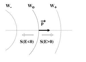
FIG. 3.: Figure.3 The wave $S(\vec{x},E,t)=W_{o}$ moves along momentum $\vec{p}$ if $E\!>\!0$ and against it if $E\!<\!0$.

Hence, the direction of a wave vector

$$\vec{k}=\nabla\Phi(\vec{x},\omega,t),$$ (A.20)

where $\Phi(\vec{x},\omega,t)$ is a wave phase, coincides with the direction of the momentum if $E\!>\!0$ and contradicts it if $E\!<\!0$

$$\left\{\begin{array}[]{l}\vec{k}\uparrow\uparrow\vec{p}\;\;\;\;E>0,\\ \\ \vec{k}\uparrow\downarrow\vec{p}\;\;\;\;E<0.\\ \end{array}\right.$$ (A.21)

Putting

$$\vec{p}=-\hbar\vec{k},$$ (A.22)

for the case $E\!<\!0$, one gets the following relation:

$$\Phi=-\frac{S}{\hbar}.$$ (A.23)

Note that the wave vector coincides with the velocity as $\vec{p}=-m\vec{v}$, and the circular frequency of the wave process is positive

$$\omega=\frac{\partial\Phi}{\partial t}=-\frac{1}{\hbar}\frac{\partial S}{\partial t}=-\frac{E}{\hbar}>0,\;\;\;\;\mbox{where}\;E<0.$$ (A.24)

Does the quantum mechanics allow a negative “action”-quantum? According to Dirac [53] the main point in quantization of a classical system is the replacement of a classical Poisson bracket by a quantum one. The latter must be Hermitian as the former is real. The minus sign in front of the Planck constant

$$\left\{A,B\right\}=\frac{1}{i(-\hbar)}(AB-BA)=-\frac{1}{i\hbar}[A,B]$$ (A.25)

does not disturb this condition. Using formulae (A.10), (A.25), one gets a commutation relation

$$[x,p]=-i\hbar,$$ (A.26)

where the momentum operator has the form

$$\hat{p}\equiv i\hbar\frac{\partial}{\partial x}.$$ (A.27)

The quasi-classical wave function reads as following according to (A.23)

$$\Psi(x,t)=\exp\left\{-\frac{i}{\hbar}S(x,t)\right\}$$ (A.28)

and must satisfy the Schrödinger equation

$$-i\hbar\frac{d}{dt}\Psi(x,t)=H(x,\hat{p})\Psi(x,t).$$ (A.29)

The energy operator changes the sign with respect to a usual case, too

$$E\to-i\hbar\frac{d}{dt}.$$ (A.30)

The Schrödinger equation (A.29) undergoes into the Hamilton –Jacoby equation (A.13) in the classical limit $\hbar\to 0$.

The probability conservation law holds

$$\frac{d\rho}{dt}+\nabla\vec{j}=0,$$ (A.31)

where

$$\rho=\Psi^{*}(x,t)\Psi(x,t),\;\;\;\;\;\vec{j}=\frac{i\hbar}{2m}\left(\Psi(x,t)\nabla\Psi^{*}(x,t)-\Psi^{*}(x,t)\nabla\Psi(x,t)\right).$$ (A.32)

The quantity $\rho$ is positive and has a meaning of the probability density under the normalizing condition

$$\int\rho dx=\int\Psi^{*}(x,t)\Psi(x,t)dx=1.$$ (A.33)

The current $\vec{j}$ coincides with the wave vector

$$\vec{j}\uparrow\uparrow\vec{k}.$$ (A.34)

The Heisenberg equations are the following:

$$\frac{d\hat{A}}{dt}=\frac{\partial\hat{A}}{\partial t}-\frac{1}{i\hbar}[\hat{A},H].$$ (A.35)

Then, according to the definition of the average of the time derivative

$$\langle\frac{d\hat{A}}{dt}\rangle=\frac{d}{dt}\langle\hat{A}\rangle,$$ (A.36)

one gets the Ehrenfest theorems

$$\left\{\begin{array}[]{l}\frac{d}{dt}\langle\hat{x}\rangle=\langle-\frac{1}{i\hbar}[\hat{x},H]\rangle=-\langle\hat{p}\rangle/m,\\ \\ \frac{d}{dt}\langle\hat{p}\rangle=\langle-\frac{1}{i\hbar}[\hat{p},H]\rangle=m\omega^{2}\langle x\rangle,\end{array}\right.$$ (A.37)

which correspond to classical Hamiltonian equations (A.11).

Now the Schrödinger picture and a filling number representation for a negative harmonic oscillator can be considered. The Schrödinger equation

$$(H-E)\Psi(x,t)=\left(-\frac{1}{2}\left(\frac{\hat{p}^{2}}{m}+m\omega^{2}x^{2}\right)-E\right)\Psi(x,t)=0,$$ (A.38)

or in coordinate representation

$$\left(\frac{\hbar^{2}}{2m}\frac{\partial^{2}}{\partial x^{2}}-\frac{1}{2}m\omega^{2}x^{2}-E\right)\Psi(x,t)=0,$$ (A.39)

differs in sign from the usual case but here the energy $E$ is less than zero. Introducing dimensionless parameters

$$\xi=\frac{x}{x_{d}},\;\;\;x_{d}=\sqrt{\frac{\hbar}{m\omega}},\;\;\;\varepsilon=\frac{-2E}{\hbar\omega}>0$$ (A.40)

we get a usual equation

$$\left(\frac{\partial^{2}}{\partial\xi^{2}}-\xi^{2}+\varepsilon\right)\Psi(x,t)=0.$$ (A.41)

Hence, the stationary states are characterized by negative energy levels

$$E_{n}=-\hbar\omega\left(n+\frac{1}{2}\right)$$ (A.42)

and by wave functions

$$\Psi_{n}(x,t)=\frac{1}{\left(\sqrt{\pi}n!2^{n}x_{d}\right)^{1/2}}\exp\left\{-\frac{1}{2}\left(\frac{x}{x_{d}}\right)^{2}\right\}H_{n}\left(\frac{x}{x_{d}}\right),$$ (A.43)

where Hermit polynomials

$$H_{n}(\xi)=(-)^{n}e^{\xi^{2}}\frac{d^{n}}{d\xi^{n}}e^{-\xi^{2}}$$ (A.44)

satisfy the orthogonality condition

$$\int\limits_{-\infty}^{+\infty}\Psi^{*}_{m}(x,t)\Psi_{n}(x,t)dx=\delta_{mn}.$$ (A.45)

To undergo to the filling number representation, let us introduce operators

$$a=\frac{1}{\sqrt{2}}\left(\xi+\frac{\partial}{\partial\xi}\right)=\frac{1}{\sqrt{2}}\left(\sqrt{\frac{m\omega}{\hbar}}x-i\frac{\hat{p}}{\sqrt{\hbar m\omega}}\right),$$ (A.46)

$$a^{\dagger}=\frac{1}{\sqrt{2}}\left(\xi-\frac{\partial}{\partial\xi}\right)=\frac{1}{\sqrt{2}}\left(\sqrt{\frac{m\omega}{\hbar}}x+i\frac{\hat{p}}{\sqrt{\hbar m\omega}}\right),$$ (A.47)

satisfying the commutation relation

$$[a,a^{\dagger}]=1$$ (A.48)

according to (A.26). The operator $a$ annuls the vacuum state

$$|0\rangle=\Psi_{o}(x,t)=\frac{1}{\pi^{1/4}}e^{-\xi^{2}/2},\;\;\;\;\langle 0|0\rangle=1,$$ (A.49)

$$a|0\rangle=0.$$ (A.50)

The operator $a^{\dagger}$ acting on to the vacuum gives exited states with the quantum number $n$

$$|n\rangle=\Psi_{n}(x,t)=\frac{1}{\sqrt{n!}}(a^{\dagger})^{n}\Psi_{o}(x,t),\;\;\;\langle n|n\rangle=1.$$ (A.51)

The energy operator looks as follows:

$$H=-\hbar\omega\left(\hat{n}+\frac{1}{2}\right),$$ (A.52)

where a particle number operator is introduced

$$\hat{n}=a^{\dagger}a,\;\;\;\;\hat{n}|n\rangle=n|n\rangle.$$ (A.53)

To give the interpretation of the operators $a,a^{\dagger}$ let us find the value of the operators $H$ and $\hat{n}$ in the stations $a^{\dagger}|n\rangle$, $a|n\rangle$

$$Ha^{\dagger}|n\rangle=(E_{n}-\hbar\omega)a^{\dagger}|n\rangle,\;\;\;\;\hat{n}a^{\dagger}|n\rangle=(n+1)a^{\dagger}|n\rangle,$$ (A.54)

$$Ha|n\rangle=(E_{n}+\hbar\omega)a|n\rangle,\;\;\;\;\hat{n}a|n\rangle=(n-1)a|n\rangle.$$ (A.55)

The operator $a^{\dagger}$ decreases the energy onto the quantity $\hbar\omega$ and increases the particle number onto a unit. This operator can be called the creation operator for the particle with the negative energy $-\hbar\omega$. The operator $a$ increases the energy onto the quantity $\hbar\omega$ and decreases the particle number onto a unit. This operator can be called the annihilation operator for the particle with the negative energy $-\hbar\omega$.

So the quantum theory of the negative energy system needs a negative “action”-quantum value by preserving the usual apparatus and probability interpretation.

B Bessel functions

The first- and second-order Hankel functions [35] are linear combinations of the Bessel functions

$$\begin{array}[]{l}H^{(1)}_{\nu}(\zeta)=J_{\nu}(\zeta)+iY_{\nu}(\zeta)\\ \\ H^{(2)}_{\nu}(\zeta)=J_{\nu}(\zeta)-iY_{\nu}(\zeta)\\ \end{array}$$ (B.1)

and satisfy the following orthogonality relation:

$$H^{(1)}_{\nu}(\zeta)\frac{d}{d\zeta}H^{(2)}_{\nu}(\zeta)-H^{(2)}_{\nu}(\zeta)\frac{d}{d\zeta}H^{(1)}_{\nu}(\zeta)=-\frac{4i}{\pi\zeta}.$$ (B.2)

They are complex conjugated by real argument $\zeta\in\Re$

$$\left(H^{(1)}_{\nu}(\zeta)\right)^{*}=H^{(2)}_{\nu}(\zeta).$$ (B.3)

The Bessel functions $J_{\frac{5}{2}}(\zeta)$ $Y_{\frac{5}{2}}(\zeta)$ can be expressed via spherical Bessel functions [35]

$$\begin{array}[]{l}j_{2}(\zeta)=\sqrt{\frac{\pi}{2\zeta}}J_{\frac{5}{2}}(\zeta)=\left(\frac{3}{\zeta^{3}}-\frac{1}{\zeta}\right)\sin(\zeta)-\frac{3}{\zeta^{2}}\cos(\zeta),\\ \\ y_{2}(\zeta)=\sqrt{\frac{\pi}{2\zeta}}Y_{\frac{5}{2}}(\zeta)=\left(-\frac{3}{\zeta^{3}}+\frac{1}{\zeta}\right)\cos(\zeta)-\frac{3}{\zeta^{2}}\sin(\zeta).\end{array}$$ (B.4)

REFERENCES

- [1] J.L. Sing, Relativity: The General Theory (Norht-Holland Publ. Comp., Amsterdam 1960).
- [2] B.S. DeWitt. Phys. Rev. 160, 1113 (1967).
- [3] W.F. Blyth, and C.J. Isham, Phys. Rev. D 11, 768 (1975).
- [4] T. Padmanabhan and J.V. Narlikar, Gen. Rel. Grav. 13, 669 (1981).
- [5] T. Padmanabhan, Phys. Rev. D 28, 745 (1983).
- [6] J.V. Narlikar and T. Padmanabhan, Phys. Rep. 100, 151 (1983).
- [7] S.W. Hawking, in General Relativity. An Einstein Centenary Survey, edited by S.W. Hawking and W. Israel (Cambridge Univ. Press, Cambridge, 1979), p. 746.
- [8] G.W. Gibbons, S.W. Hawking, and M.J. Perry, Nucl. Phys. B138, 141 (1978).
- [9] K. Schleich, Phys. Rev. D 36 2342 (1987).
- [10] A.D. Linde, Zh. Éksp. Teor. Fiz. 87, 369 (1984) [Sov. Phys. JETP 60, 211 (1984)].
- [11] S. Weinberg, Gravitation and Cosmology: Principles and Applications of the General Theory of Relativity (New York: Wiley, 1972).
- [12] M. Ryan, Hamiltonian Cosmology, Lecture Notes in Physics N 13, (Springer-Verlag, Berlin, 1972).
- [13] T. Padmanabhan, Gen. Rel. Grav. 15, 435 (1983).
- [14] T. Padmanabhan, Gen. Rel. Grav. 19, 927 (1987).
- [15] S. Perlmutter et al., Astrophys. J. 517, 565 (1999). A.G. Riess at al., The Astronom. J. 116, 1009 (1998).
- [16] S. Weinberg, Rev. Mod. Phys. 61, 1 (1989).
- [17] E.W. Kolb, M.S. Turner, The Early Universe, Frontiers in Physics 69 (Addison Wesley Publ. Comp., 1990).
- [18] P.F. González-Díaz, Phys. Rev. D 62, 023513 (2000).
- [19] A.R.Liddle and D.H. Lyth, Phys. Rep. 231, 1 (1993). D.H. Lyth and A. Riotto, Phys. Rep. 314, 1 (1999).
- [20] J.J. Halliwell and S.W. Hawking, Phys. Rev. D 31, 1777 (1985).
- [21] R.H. Sachs and A.M. Wolfe, Astroph. J. 147, 73 (1967).
- [22] D. Boyanovsky, H.J. de Vega, R. Holman, and J. Salgado, Phys. Rev. D 59, 125009 (1999).
-
[23]
O. Éboli, R. Jackiw, and So-Young Pi,
Phys. Rev. D 37, 3557 (1988).
R. Jackiw, Analysis on infinite-dimensional manifolds – Schrödinger representation for quantized fields, Séminare de Mathématiques Supérieures, Montréal, Québec, Canada, June 1988 and V Jorge Swieca Summer School, São Paulo, Brazil, January 1989, CTP#1720 March 1989. - [24] N.A. Chernikov, and E.A. Tagirov, Ann. Inst. H. Poincaré 9A, 109 (1968).
- [25] L.D. Landau, and E.M. Lifshitz, Classical Theory of Fields (Pergamon Press, Oxford, 1975).
- [26] C.W. Misner, K. Thorne, and J.A. Wheeler, Gravitation (Freeman, San Francisco 1973).
- [27] L.P. Eisenhart, Riemannian Geometry (Princeton University, Princeton 1926).
- [28] A.P. Lightman, W.H. Press, R.H. Price, S.A. Teukolsky, Problem book in Relativity and Gravitation (Princeton Univ. Press, Princeton, New Jersey 1975).
- [29] A.J. Keane, and R.K. Barrett, Class. Quantum Grav. 17, 201 (2000).
- [30] B.A. Dubrovin, S.P. Novikov, and A.T. Fomenko, Modern Geometry Methods and Applications, Part II, The Geometry and Topology of Manifold (Springer Verlag , New York 1984).
- [31] F. Gürsey, in Relativity, Groups and Topology, edited by C. DeWitt and B. DeWitt (New York, London 1964), p. 91.
- [32] A.H. Guth and So-Young Pi, Phys. Rev. D 32, 1899 (1985).
- [33] T.S. Bunch and P.C.W. Davies, Proc. R. Soc. Lond. A 360, 117 (1978).
- [34] R. Floreanini, C.T. Hill, and R. Jackiw, Ann. Phys. (N.Y.) 175, 345 (1987).
- [35] Handbook of Mathematical Functions edited by M Abramowitz and I.A. Stegun (Dover, New York 1965).
- [36] V.F. Mukhanov, H.A. Feldman, and R.H. Branderberger, Phys. Rep. 215, 203 (1992).
- [37] H.A. Lorentz, Amst. Versl., Bd 23, 1073 (1915), Bd 24, 1389 and 1759 (1916), Bd 25, 468 and 1380 (1916).
- [38] T. Levi-Civita, ensteiniani in campi newtoniani. I-IX// Rend. Acc. Linc. (5). Bd 26 (1917), Bd 27 (1918), Bd 28 (1919).
- [39] P.A.M. Dirac, Canad. J. Math. 2, 129 (1950); Canad. J. Math. 3, 1 (1951); Proc. Roy. Soc. A246, 326 (1958).
- [40] S.S. Schweber, An Introduction to Relativistic Quantum Field Theory (Harper and Row, N.Y. 1961).
- [41] S.W. Hawking, G.F.R. Ellis, The Large Scale Structure of Space-Time (Cambridge, Cambridge University Press, 1973).
- [42] J.B. Hartle, S.W. Hawking, Phys. Rev. D 28, 2960 (1983).
- [43] A. Vilenkin, Phys. Rev. D 37, 888 (1988).
- [44] R.R. Caldwell, astro-ph/9908168.
- [45] T. Chiba, T. Okabe, and M. Yamaguchi, Phys. Rev. D 62, 023511 (2000).
- [46] J.V. Narlikar, T. Padmanabhan, Annu. Rev. Astron. Astrophys. 29, 325 (1991).
- [47] W. Thirring, Ann. of Phys. (N.Y.) 16, 96 (1961).
- [48] N. Rosen, Phys. Rev. 57, 147 and 150 (1940).
- [49] A. Papapetrou, Proc. R. Irish Acad. A52, 11 (1948).
- [50] C. Fronsdal, Nuovo Chimento Suppl. 9, 416 (1958).
- [51] K.J. Barnes, J. Math. Phys. 6, 788 (1965).
- [52] H. Goldstein, Classical Mechanics (Addison-Wesley Press, INC. Cambridge. Mass. 1950).
- [53] P.A.M. Dirac, The Principles of Quantum Mechanics (Oxford at the Clarendon Press 1958).