Oscillatory approach to the singularity in vacuum spacetimes with $T^{2}$ isometry

Abstract

We use qualitative arguments combined with numerical simulations to argue that, in the approach to the singularity in a vacuum solution of Einstein’s equations with $T^{2}$ isometry, the evolution at a generic point in space is an endless succession of Kasner epochs, punctuated by bounces in which either a curvature term or a twist term becomes important in the evolution equations for a brief time. Both curvature bounces and twist bounces may be understood within the context of local mixmaster dynamics although the latter have never been seen before in spatially inhomogeneous cosmological spacetimes.

04.20.Dw,98.80.Dr

I Introduction

Thirty years ago, Misner [1] and Belinskii, Khalatnikov and Lifshitz (BKL) [2] noted that Bianchi IX spatially homogeneous cosmological solutions of Einstein’s equations seem to exhibit a sort of oscillatory behavior in the approach to the singularity. This behavior, labeled “mixmaster” [1], involves an infinite sequence of periods (or “epochs”) during which the solution evolves essentially as a Kasner spacetime [3, 4], with each Kasner epoch ended by a “bounce” of short duration which changes the evolution from that of one Kasner to that of another one. The sequence of Kasners satisfies a rule, called the Kasner map, which takes one Kasner in the sequence to the next. This characterization of the Bianchi IX singularity has recently been made rigorous [5]. BKL also made the rather surprising claim [2, 6] that in spatially inhomogeneous solutions of Einstein’s equations, timelike observers approaching a Big Bang or Big Crunch singularity should generally see this oscillatory behavior, with the Kasner epoch seen by one observer differing from that seen by other neighboring observers, but the sequence of Kasners for each observer still satisfying the Kasner map.

Our previous study of the magnetic Gowdy family of spacetimes [8] provided the first firm support for BKL’s claim in a spatially inhomogeneous setting. In that work, we numerically evolve spacetimes in the family using the standard areal (or “Gowdy”) time foliation, and we find that generic observers see oscillatory behavior in the metric evolution. Moreover, our studies of the magnetic Gowdy spacetimes indicate that the sequence of Kasners seen by each observer follow the pattern of succession predicted by BKL [2, 6]. Further, these studies agree with the qualitative picture which the Grubišić-Moncrief method of consistent potentials (MCP) suggests [9].

Since this magnetic Gowdy work, numerical and MCP studies of two other families of cosmological spacetimes have been carried out: the $T^{2}$ symmetric vacuum spacetimes and the $U(1)$ symmetric vacuum spacetimes. Both studies strongly support the BKL claim that the approach to the singularity is oscillatory. The results for $U(1)$ symmetric solutions have been reported elsewhere [10]. Here, we discuss the behavior near the singularity for $T^{2}$ symmetric vacuum spacetimes.

Since $U(1)$ is a subgroup of $T^{2}=U(1)\times U(1)$, the $T^{2}$ symmetric vacuum spacetimes are a subfamily of the $U(1)$ symmetric vacuum spacetimes. One may then ask why it is useful to study the $T^{2}$ symmetric family directly. The reason is that, since the equations for the $T^{2}$ symmetric family are considerably simpler (1+1 PDEs rather than 2+1 PDEs) the numerical studies can be done significantly more accurately. Hence, the studies are more accurate for the $T^{2}$ symmetric family, and the behavior of the bounces seen by the observers can be monitored more carefully. The MCP analysis has been carried out in great detail in this simpler case. We report this study here both to present the detailed picture it gives of the dynamics in these spacetimes, and also, we hope, as an aid to obtaining rigorous results about the dynamics.

We define the $T^{2}$ symmetric family in Sec. II, noting the relationship between this family and others, such as the Gowdy [11] and the Kasner spacetimes. Also in Sec. II, we discuss the areal function and coordinates, recalling results which justify their use for $T^{2}$ symmetric solutions and writing out the field equations. In Sec. III, we set up the MCP treatment of the evolution equations for the $T^{2}$ symmetric spacetimes and use it to argue that oscillatory behavior occurs. We recall that in setting up the MCP form of a given set of evolution equations, one presumes that at each spatial point, the fields evolve to Kasner epoch values (not necessarily at the same time for all spatial points); one then substitutes these Kasner-like values of the fields into the right hand side of the evolution equations, and attempts to infer how the various terms in these equations should behave in time, and what the resulting behavior of the fields should be. This analysis predicts that there should be three types of bounces in $T^{2}$ symmetric spacetimes: curvature bounces, twist bounces and kinetic bounces. A kinetic bounce is not a transition between two distinct Kasner epochs. Rather, it occurs within a Kasner epoch. However, in terms of the evolution of the metric functions, it is a bounce on a par with the others and its occurrence is necessary for the oscillatory behavior to continue. We state in Appendix A the explicit evolution of the fields during each of the three bounces (ignoring in each case terms in the evolution equations which are small) and discuss the qualitative nature of each in Sec. III. We compare the MCP predictions for bounce behavior with those of BKL. We also discuss in Sec. III the MCP argument that, in these spacetimes, an observer following a timelike path of constant spatial coordinate should see an unending succession of bounces, a key ingredient of mixmaster dynamics and the BKL claims.

MCP analysis provides useful predictions, but is limited in that, besides being nonrigorous, it does not predict whether generic initial data will evolve into a spacetime in which, along each appropriate timelike observer’s path, a Kasner-like state is reached. (This, again, is a prerequisite for carrying out the MCP study.) To justify the MCP predictions, we rely on numerical studies of $T^{2}$ symmetric solutions. For representative sets of initial data, Kasner epoch values for the fields are reached at each spatial point. Once the Kasner regime is reached at a given spatial point, the bounces occur as predicted by our MCP studies, as far as we are able to carry out the evolution. Discussion of these results is presented in Sec. IV. These numerical studies do not prove that $T^{2}$ symmetric solutions generically exhibit oscillatory behavior near the singularity, as predicted by BKL. They do, however, strongly support this contention.

In the magnetic Gowdy family of spacetimes, we have found that in a generic solution, conditions can occur at nongeneric spatial points (e.g., the derivative of a metric component has a zero) with the result that at various points near this nongeneric point, there is only a finite number of bounces. While similar conditions occur at nongeneric spatial points in a generic $T^{2}$ symmetric solution, and while these conditions again appear to persist, there is as yet no evidence that the bounces stop at nearby points, in contrast to the situation in a magnetic Gowdy solution. The occurrence of the exceptional points is observed in the numerical simulations, and the long time behavior is predicted by the MCP analysis. We discuss and exhibit exceptional points in Sections III and IV, but leave extensive discussion of these to future work [12]. We make concluding remarks in Sec. V.

II The $T^{2}$ symmetric spacetimes

We define the $T^{2}$ symmetric family of spacetimes to consist of globally hyperbolic solutions of the vacuum Einstein equations with compact Cauchy surfaces and with a $T^{2}$ isometry group acting spatially and without fixed points. Generally for spacetimes in this family, at least one of the “twist” functions

$$K_{(X)}\,:=\epsilon_{\mu\nu\rho\lambda}X^{\mu}Y^{\nu}\nabla^{\rho}X^{\lambda}\hskip 20.0pt\mbox{ and }\hskip 20.0ptK_{(Y)}\,:=\epsilon_{\mu\nu\rho\lambda}X^{\mu}Y^{\nu}\nabla^{\rho}Y^{\lambda}$$ (1)

does not vanish. (Here $X$ and $Y$ are a pair of Killing fields which generate the $T^{2}$ isometry group.) If in fact both twist functions do vanish, then one obtains the important subfamily of Gowdy spacetimes.

The Gowdy spacetimes have been extensively studied, and it is believed[9, 13, 14, 15, 16, 17, 18, 19] that they are all Asymptotically Velocity Term Dominated (AVTD). Roughly speaking, this means that as each observer in a given spacetime approaches the singularity, she sees at most a finite number of bounces, and eventually settles into a final Kasner epoch which generally varies from point to point. Since the Gowdy spacetimes are fairly well understood, and since they are a set of measure zero in the full family of $T^{2}$ symmetric spacetimes, we shall henceforth presume that one or both of the twist functions is nonzero, in which case the only topology compatible with $T^{2}$ symmetric spacetimes is $T^{3}\times{\mathcal{R}}^{1}$.

It is very useful in studying the properties of the evolution in a given family of spacetimes to have available a universal choice of spacetime foliation which exactly covers the maximal globally hyperbolic development of every spacetime in that family. As proven in [21], the “areal foliation” (with corresponding areal coordinates) serves this purpose for the $T^{2}$ symmetric solutions. We recall that the areal foliation chooses spacelike hypersurfaces which are invariant under the $T^{2}$ action (thereby containing complete orbits of $T^{2}$) with each leaf of the foliation consisting of all orbits of a fixed area. That is, if we let $R:T^{3}\times{\mathcal{R}}^{1}\rightarrow{\mathcal{R}}^{1}$ be the function which assigns to a given spacetime point the area of the $T^{2}$ orbit which contains that point, then the areal foliation chooses for its time function some $t\propto R$. In [21] (see also [22]), it is shown that for every $T^{2}$ symmetric solution $(T^{3}\times{\mathcal{R}},g)$ of the vacuum Einstein equations, (i) such a function $t$ is indeed timelike, (ii) for every value of $t\in(t_{0},\infty)$ with $t_{0}>0$ ($t_{0}$ fixed for each spacetime) the $t$ leaf is indeed a $T^{3}$ Cauchy surface and (iii) the $t$-hypersurfaces, with $t\in(t_{0},\infty)$, collectively cover the maximal globally hyperbolic region of $(T^{3}\times{\mathcal{R}},g)$. Hence, the areal foliation provides the desired universal choice of time for the $T^{2}$ symmetric spacetimes. We note that for the Gowdy spacetimes, $t$ is the familiar Gowdy time.

If we use $(x,y)\in T^{2}$ as coordinates labeling points on the $T^{2}$ isometry group orbits, and use $\theta\in S^{1}$ as a coordinate parametrizing distinct orbits, then ${(\theta,x,y,t)}$ serve as universal coordinates for the $T^{2}$ symmetric spacetimes, and we may write the generic metric for this family in the form

$$g = e^{2(\nu-U)}(-\alpha\,dt^{2}+d\theta^{2})$$ (4)

$$\;\;+\sigma\,e^{2U}[dx+A\,dy+(G_{1}+A\,G_{2})\,d\theta+(M_{1}+A\,M_{2})\,dt]^{2}$$

$$\;\;+\sigma\,e^{-2U}t^{2}[dy+G_{2}\,d\theta+M_{2}\,dt]^{2}$$

where $U$, $A$, $\nu$, $\alpha$, $G_{1}$, $G_{2}$, $M_{1}$ and $M_{2}$ are functions of $\theta$ and $t$ (independent of $x$ and $y$), and $\sigma$ is a positive constant. This form (4) for the $T^{2}$ symmetric metrics is used for the analysis in [21]. Here, to make it easier to compare the present study of $T^{2}$ symmetric spacetimes with previous similar studies of magnetic Gowdy spacetimes [8] and Gowdy spacetimes [13, 14, 15, 23], it is useful to replace the time function $t$ by $\tau=-\ln t$ (one still has an areal type foliation) and the metric functions $U$, $A$, $\nu$ and $\alpha$ by the following equivalent functions.

$$P = 2\,U+\tau\,,$$ (5)

$$Q = A\,,$$ (6)

$$\mu = -2\ln\alpha\,,$$ (7)

$$\lambda = 4\,\nu-4\,U+2\ln\alpha-\tau\,.$$ (8)

In terms of these variables, the metric takes the form

$$g = -e^{(\lambda-3\tau)/2}d\tau^{2}+e^{(\lambda+\mu+\tau)/2}d\theta^{2}$$ (11)

$$\;\;+\sigma\,e^{P-\tau}[dx+Q\,dy+(G_{1}+Q\,G_{2})\,d\theta+(M_{1}+Q\,M_{2})\,(-e^{-\tau}d\tau)]^{2}$$

$$\;\;+\sigma\,e^{-P-\tau}[dy+G_{2}\,d\theta+M_{2}\,(-e^{-\tau}d\tau)]^{2}.$$

We note, for purposes of comparison, that the metric for magnetic Gowdy spacetimes is the same as (11) except that $G_{1}$, $G_{2}$, $M_{1}$ and $M_{2}$ vanish. If one relaxes the assumption of the $T^{2}$ isometry to allow it to be a local isometry, then other spatial topologies in addition to $T^{3}$ are possible in the magnetic case or the Gowdy case but not in the general $T^{2}$ symmetric case with nonvanishing twist. The topology affects the spatial boundary conditions of the functions $P$ and $Q$, but not the qualitative behavior of the evolution toward the singularity [12, 16, 24].

The Einstein vacuum field equations for the $T^{2}$ symmetric spacetimes [21] naturally divide themselves into four sets. The first set

$$\partial_{\theta}K_{(X)}\,=0\hskip 20.0pt,\hskip 20.0pt\partial_{\tau}K_{(X)}\,=0\hskip 20.0pt,\hskip 20.0pt\partial_{\theta}K_{(Y)}\,=0\hskip 20.0pt,\hskip 20.0pt\partial_{\tau}K_{(Y)}\,=0$$ (12)

simply tells us that the twist functions are constant in space and time (and hence are labeled the “twist constants”). For any given $T^{2}$ symmetric spacetime, we may always replace $X$ and $Y$ by a linear combination of themselves and thereby cause one or the other twist functions to vanish (but not both). Hence, without loss of generality, we may further presume that only one of the twist constants is nonzero. We label it $K$.

The next two sets are the constraint equations and the evolution equations for the metric functions $\{P,Q,\mu,\lambda\}$. They involve the twist constant $K$, but are independent of $\{G_{1},G_{2},M_{1},M_{2}\}$. We discuss these equations below. The last set of equations govern $\{G_{1},G_{2},M_{1},M_{2}\}$. They take the form

$$\partial_{\tau}G_{1} = -e^{-\tau}\partial_{\theta}M_{1}+Q\,e^{(\mu+2\lambda+4P+6\tau)/4}K\,,$$ (13)

$$\partial_{\tau}G_{2} = -e^{-\tau}\partial_{\theta}M_{2}-e^{(\mu+2\lambda+4P+6\tau)/4}K.$$ (14)

We see from these equations that, once $\{P,Q,\mu,\lambda\}$ have been determined, one obtains $\{G_{1},G_{2},M_{1},M_{2}\}$ by choosing $M_{1}(\theta,\tau)$ and $M_{2}(\theta,\tau)$ to be arbitrary functions of $\theta$ and $\tau$, choosing $\hat{G}_{1}(\theta)$ and $\hat{G}_{2}(\theta)$ as arbitrary (initial data) functions on $S^{1}$ and then integrating Eqs. (13) – (14) over $\tau$ to get $G_{1}(\theta,\tau)$ and $G_{2}(\theta,\tau)$. Thus $\{G_{1},G_{2},M_{1},M_{2}\}$ are nondynamical fields. They are essentially “shift functions”, which determine how the coordinates $(x,y)$ evolve in $\tau$ and $\theta$. If $K$ is nonvanishing, $\{G_{1},G_{2},M_{1},M_{2}\}$ cannot all vanish everywhere in spacetime; the symmetry group does not act orthogonally transitively [25].

The dynamics of the gravitational field in $T^{2}$ symmetric spacetimes lie in $\{P,Q,\mu,\lambda\}$. To study these fields we find it useful to work in Hamiltonian form. Letting $\pi_{P}$, $\pi_{Q}$, $\pi_{\mu}$ and $\pi_{\lambda}$ denote the momenta conjugate to these four fields, we find that $\pi_{\mu}$ may be eliminated, that the functions $\{P,Q,\mu,\lambda,\pi_{P},\pi_{Q},\pi_{\lambda}\}$ must satisfy the constraint equations

$$\pi_{\lambda}-{1\over 2}e^{\mu\over 4} = 0\,,$$ (15)

$$\pi_{P}\,\partial_{\theta}P+\pi_{Q}\,\partial_{\theta}Q+\pi_{\lambda}\,\partial_{\theta}\lambda = 0$$ (16)

and that the evolution equations for $\{P,Q,\lambda,\pi_{P},\pi_{Q},\pi_{\lambda}\}$ can be obtained by varying the Hamiltonian density

$$H={1\over 4\pi_{\lambda}}\biggl{[}\pi_{P}^{2}+e^{-2P}\pi_{Q}^{2}+e^{-2\tau}(\partial_{\theta}P)^{2}+e^{2(P-\tau)}(\partial_{\theta}Q)^{2}\biggr{]}+\sigma\,\pi_{\lambda}e^{{(\lambda+2P+3\tau)/2}}K^{2}.$$ (17)

In particular we have

$$\partial_{\tau}P = {\pi_{P}\over 2\pi_{\lambda}}\,,$$ (19)

$$\partial_{\tau}\pi_{P} = {1\over 2\pi_{\lambda}}[e^{-2P}\pi_{Q}^{2}+e^{-2\tau}\partial_{\theta\theta}P-{e^{-2\tau}(\partial_{\theta}P)(\partial_{\theta}\pi_{\lambda})\over\pi_{\lambda}}-e^{2(P-\tau)}(\partial_{\theta}Q)^{2}]$$ (21)

$$\hskip 144.54pt-\sigma\,\pi_{\lambda}e^{{(\lambda+2P+3\tau)/2}}K^{2}\,,$$

$$\partial_{\tau}Q = {e^{-2P}\pi_{Q}\over 2\pi_{\lambda}}\,,$$ (22)

$$\partial_{\tau}\pi_{Q} = {e^{2(P-\tau)}\over 2\pi_{\lambda}}[\partial_{\theta\theta}Q-{(\partial_{\theta}Q)(\partial_{\theta}\pi_{\lambda})\over\pi_{\lambda}}+2(\partial_{\theta}P)(\partial_{\theta}Q)]\,,$$ (23)

$$\partial_{\tau}\lambda = -{1\over(2\pi_{\lambda})^{2}}[\pi_{P}^{2}+e^{-2P}\pi_{Q}^{2}+{e^{-2\tau}(\partial_{\theta}P)^{2}+e^{2(P-\tau)}(\partial_{\theta}Q)^{2}]}$$ (25)

$$\hskip 144.54pt+\sigma\,e^{{(\lambda+2P+3\tau)/2}}K^{2}\,,$$

$$\partial_{\tau}\pi_{\lambda} = -{1\over 2}\sigma\,\pi_{\lambda}e^{(\lambda+2P+3\tau)/2}K^{2}\,.$$ (26)

The evolution for the remaining metric function, $\mu$, follows from the constraint (15)

$$\partial_{\tau}\mu=-2\sigma\,e^{(\lambda+2P+3\tau)/2}K^{2}.$$ (27)

The constraint equations, the Hamiltonian and the evolution equations for the fields for magnetic Gowdy spacetimes are very similar to these; the main difference is that the twist terms in the Hamiltonian density and in the evolution equations are replaced by magnetic terms, with the exponential coefficient for the magnetic terms, $e^{(\lambda+\tau)/2}$, differing from that for the twist terms, $e^{(\lambda+2P+3\tau)/2}$. This difference leads to interesting consequences, which we discuss in a future work [12].

We have already noted the relationship between the familiar Gowdy spacetimes and the $T^{2}$ symmetric spacetimes discussed here. The (locally) spatially homogeneous subfamily of the Gowdy spacetimes consists of the Kasner spacetimes. The (locally) spatially homogeneous subfamily of the generic $T^{2}$ symmetric spacetimes, with non-vanishing twist, consists of Kasner spacetimes as well. This may seem surprising, since for the standard Kasner Killing vectors, all the twist functions vanish. However, one verifies that, in the locally homogeneous subfamily, $X$ and $Y$ (with nonvanishing twist) are a linear combination (with constant coefficients) of the three Kasner Killing vector fields. The coefficients are constant, but since the norms are changing in time, the angles between the two sets of Killing vectors are changing in time. More specifically, consider two orthonormal spatial bases: $E_{i}$, made up of eigenvectors of the extrinsic curvature (the Kasner directions), and $e_{i}$, such that each vector in the frame is proportional to a (local) Killing vector and such that two of the frame vectors are tangent to the isometry orbits generated by $X$ and $Y$. Then the relation between the two frames is a time dependent rotation.

Another subfamily of the $T^{2}$ symmetric spacetimes is worth noting. If one chooses initial data with $Q(\theta,\tau_{0})=0$ and $\pi_{Q}(\theta,\tau_{0})=0$, then $Q(\theta,\tau)=0$ and $\pi_{Q}(\theta,\tau)=0$ for all points in the spacetime development of this data. (See equations (22) and (23).) Hence, one can consider a subfamily, the “polarized” $T^{2}$ symmetric spacetimes, with the metric coefficient $Q$—and the corresponding gravitational degree of freedom—turned off. The polarized $T^{2}$ symmetric spacetimes have been studied using Fuchsian methods, and one finds [26] that there are full-parameter sets of these which are AVTD rather than oscillatory near the singularity. Thus although oscillatory behavior is expected to occur generically in $T^{2}$ symmetric spacetimes, it is not expected to occur in either the Gowdy or the polarized subfamilies.

III MCP argument for oscillatory behavior

The method of consistent potentials (MCP) is a systematic approximation scheme [27] for predicting the behavior of cosmological solutions of Einstein’s equations in the neighborhood of their singularities. It is based on a key assumption, which in practice must be checked numerically. The consequence of this assumption is a weighting of the influence of various terms in the Hamiltonian. To describe this, it is useful to split the Hamiltonian density (17) as follows:

$$H=H_{0}+H_{kin}+H_{small}+H_{curv}+H_{twist}$$ (28)

where

$$H_{0} = {1\over 4\pi_{\lambda}}\pi_{P}^{2}\,,$$ (28)

$$H_{kin} = {1\over 4\pi_{\lambda}}e^{-2P}\pi_{Q}^{2}\,,$$ (29)

$$H_{small} = {1\over 4\pi_{\lambda}}e^{-2\tau}(\partial_{\theta}P)^{2}\,,$$ (30)

$$H_{curv} = {1\over 4\pi_{\lambda}}e^{2(P-\tau)}(\partial_{\theta}Q)^{2}\,,$$ (31)

$$H_{twist} = \sigma\,\pi_{\lambda}e^{{(\lambda+2P+3\tau)/2}}K^{2}\,.$$ (32)

The assumption, for a fixed $T^{2}$ symmetric vacuum solution $(T^{3}\times{\cal R},g)$ with the singularity at $\tau\rightarrow\infty$, concerns the momentary values of the fields for large $\tau$.

Kasner Epoch Assumption (KEA):   For each $\theta\in S^{1}$, there exists a time $\tau_{(\theta)}$ such that

$$-\tau_{(\theta)}\ll 0,$$ (35)

$$-P(\theta,\tau_{(\theta)})\ll 0,$$ (36)

$$P(\theta,\tau_{(\theta)})-\tau_{(\theta)}\ll 0,$$ (37)

$$\lambda(\theta,\tau_{(\theta)})+2P(\theta,\tau_{(\theta)})+3\tau_{(\theta)}\ll 0,$$ (38)

such that

$$H_{0} \gg H_{kin},$$ (40)

$$H_{0} \gg H_{small},$$ (41)

$$H_{0} \gg H_{curv},$$ (42)

$$H_{0} \gg H_{twist},$$ (43)

and such that the terms in the evolution equations due to $H_{0}$ dominate the terms in the evolution equations due to $H_{kin}$, $H_{small}$, $H_{curv}$ and $H_{twist}$.

Explicitly, this assumption says that for each $\theta$-labeled observer in the spacetime, there is a time $\tau_{(\theta)}$ such that all of the exponential factors in the Hamiltonian density at $(\theta,\tau_{(\theta)})$ are very small. (The same factors also appear in the evolution equations.) This follows from the conditions (35)–(38). In addition, this assumption says that at this time the fields $\{P,Q,\lambda,\pi_{P},\pi_{Q},\pi_{\lambda}\}$ have developed in such a way that the exponential factors control the relative size of the various terms in the Hamiltonian density and also in the evolution equations.

The intent of the KEA is to say that, in any of these spacetimes, the evolution proceeds in such a way that each of the $\theta$ = constant observers will, at some time $\tau_{(\theta)}$ (generally varying from point to point) reach a Kasner epoch. This follows immediately from the evolution equations under the conditions assumed. One might worry that it is too restrictive to require that $H_{0}$ dominate the other terms in the Hamiltonian density, because it is possible that $H_{0}$ vanishes during a Kasner epoch, but then the prediction of the MCP analysis is that $H_{0}$ will dominate the other terms in the next Kasner epoch occurring at that value of $\theta$, so the KEA will thus be satisfied in this next Kasner epoch.

A consequence of the KEA, combined with the MCP analysis, is that generally (the exceptions are briefly discussed later in this Section) the fields evolve in such a way that they do not counteract any explicit exponential decay or growth of $H_{kin}$, $H_{curv}$ or $H_{twist}$, or that of terms in the evolution equations (LABEL:eveq) derived from $H_{kin}$, $H_{curv}$ or $H_{twist}$. That is, besides dominating the relative size of the various terms in the Hamiltonian density (17) and in the evolution equations (19)–(26), the exponential terms dominate the changes in relative size of the terms. So, for example, if $\lambda(\theta,\tau_{(\theta)})+2P(\theta,\tau_{(\theta)})+3\tau_{(\theta)}\ll 0$ and ${d\over d\tau}(\lambda(\theta,\tau_{(\theta)})+2P(\theta,\tau_{(\theta)})+3\tau_{(\theta)})|_{(\theta,\tau_{(\theta)})}>0$, then it follows from the KEA that $H_{twist}$ is small relative to $H_{0}$ at $(\theta,\tau_{(\theta)})$, and it follows from this assumption combined with the evolution equations that $H_{twist}$ is growing in $\tau$.

Numerical results, which we discuss in Sec. IV, indicate that the KEA holds for $T^{2}$ symmetric solutions.

We now consider what happens to the gravitational fields along a fixed $\theta$ observer path after a Kasner epoch has begun at some time $\tau_{(\theta)}$. We presume a fixed spacetime, and we assume the KEA discussed above. Examining the evolution equations (19)–(26), we find that the right hand sides of all but (19) and (25) are extremely small. Hence the variables $\{Q,\mu,\pi_{P},\pi_{Q},\pi_{\lambda}\}$ are essentially constant. The variables $P$ and $\lambda$ are not constant; but if we set

$$w:={\pi_{P}\over 2\pi_{\lambda}}$$ (44)

we have

$$\partial_{\tau}P=w$$ (45)

and

$$\partial_{\tau}\lambda=-w^{2}+{\cal O}$$ (46)

where $\cal O$ indicates terms which, as a consequence of the KEA, can be neglected. The function $w$ is essentially constant, so $P$ and $\lambda$ evolve linearly with $\tau$. Since all four Hamiltonian potentials, $\{H_{kin},H_{small},H_{curv},H_{twist}\}$ are negligible, we call the evolution “velocity dominated” when a) the KEA holds, b) $\{Q,\mu,\pi_{P},\pi_{Q},\pi_{\lambda}\}$ are essentially constant (note that this implies that $w$ is essentially constant), and c) $\partial_{\tau}\lambda\approx-(\partial_{\tau}P)^{2}=-w^{2}$. To reiterate, part a) implies parts b) and c), that is, the KEA implies that the evolution is velocity dominated at $\tau_{(\theta)}$.

This predicted pattern of evolution for the variables $\{P,Q,\lambda,\mu,\pi_{P},\pi_{Q},\pi_{\lambda}\}$ and their spatial derivatives, none increasing or decreasing faster than linearly, is consistent with the KEA. The conditions in the assumption continue to hold so long as the Hamiltonian potentials stay small relative to $H_{0}$. To see whether or not these potentials do indeed stay small for $\tau>\tau_{(\theta)}$ at $\theta$, we need to examine the time derivatives of the exponential quantities in the expressions (28) for $H_{kin}$, $H_{small}$, $H_{curv}$ and $H_{twist}$. We have

$$\partial_{\tau}(-2P) = -2w,$$ (48)

$$\partial_{\tau}(-2\tau) = -2,$$ (49)

$$\partial_{\tau}(2P-2\tau) = 2(w-1),$$ (50)

$$\partial_{\tau}\left[{1\over 2}\left({\lambda+2P+3\tau}\right)\right] = -{1\over 2}w^{2}+w+{3\over 2},$$ (51)

with $w$ approximately constant in $\tau$. Clearly the value of the quantity $w$ is crucial in determining whether each of the potentials grows or not. In particular, we have, at fixed $(\theta,\tau_{(\theta)})$,

$$H_{kin}\;\;\mbox{grows if}\;\;w<0\;\;(\mbox{and}\;\;\pi_{Q}\neq 0),$$ (53)

$$H_{small}\;\;\mbox{decays}\;\;(\mbox{if}\;\;\partial_{\theta}P\neq 0),$$ (54)

$$H_{curv}\;\;\mbox{grows if}\;\;w>0\;\;(\mbox{and}\;\;\partial_{\theta}Q\neq 0),$$ (55)

$$H_{twist}\;\;\mbox{grows if}\;\;-1<w<3.$$ (56)

Stating this another way, we have the results listed in Table I. Note that the conditions within the parentheses in equations (53)–(55) ensure “generic” behavior.

It does not follow from Table I that if the KEA holds there must be at least one growing potential at $(\theta,\tau_{(\theta)})$. To argue that, we need to assume that both $\pi_{Q}$ and $\partial_{\theta}Q$ are nonzero at $(\theta,\tau_{(\theta)})$. Since generally these smooth functions, $\pi_{Q}$ and $\partial_{\theta}Q$, are nonzero at a given $(\theta,\tau)$, we define $(\theta,\tau_{(\theta)})$ to be generic if neither vanishes, and exceptional if one of them does vanish. Exceptional behavior (of a different type, to be discussed later) also occurs if $w=1$. Our subsequent discussion presumes that $(\theta,\tau_{(\theta)})$ is generic unless explicitly stated otherwise; we discuss the exceptional cases briefly below and in more detail in [12].

Assuming genericity, it does follow from Table I that, during velocity dominated evolution, at least one of the potentials is growing. Indeed, the growth is exponential in $\tau$. To see what affect this has, we need to consider how the fields evolve with one or more of the potentials $H_{kin}$, $H_{curv}$ and $H_{twist}$ turned on and hence added to $H_{0}$.

In discussing what happens when some of the potentials become significant, it is useful to keep track of the generalized Kasner exponents. These are defined to be the eigenvalues of the extrinsic curvature, divided by the mean curvature. It follows from the definition that the sum of the three generalized Kasner exponents equals $1$. Defining the quantity [9, 13, 14, 15]

$$v:={1\over 2\pi_{\lambda}}(\pi_{P}^{2}+e^{-2P}\pi_{Q}^{2})^{1\over 2},$$ (57)

the generalized Kasner exponents for a $T^{2}$ symmetric solution are

$$\kappa_{1}={v^{2}-1\over v^{2}+3}+{\cal O}\;\;\;\;,\;\;\;\;\kappa_{2}={2-2v\over v^{2}+3}+{\cal O}\;\;\;\;,\;\;\;\;\kappa_{3}={2+2v\over v^{2}+3}+{\cal O}.$$ (58)

As before, $\cal O$ indicates terms which can be neglected at $(\theta,\tau_{(\theta)})$ when the KEA is satisfied, as shown in Appendix B. Note that the KEA implies $v\approx|\pi_{P}|/2\pi_{\lambda}=|w|$, and therefore that the generalized Kasner exponents are essentially constant in time. And furthermore, considering the expressions (58), we see that, in addition to $\kappa_{1}+\kappa_{2}+\kappa_{3}=1$ which always is satisfied, when the KEA holds it is also the case that $\kappa_{1}^{2}+\kappa_{2}^{2}+\kappa_{3}^{2}\approx 1$. These are the necessary and sufficient conditions that a set of three numbers be a set of Kasner exponents. Thus the generalized Kasner exponents are approximately a set of Kasner exponents when the KEA holds, and so the KEA does indeed imply that the evolution is essentially Kasner at $(\theta,\tau_{(\theta)})$.

We recall that the BKL parameter “$u$” summarizes the information in a set of Kasner exponents [2, 6]. Except for the case $\{0,0,1\}$, there always exists a $u\geq 1$ such that

$$\kappa_{min}={-u\over 1+u+u^{2}}\;\;\;\;,\;\;\;\;\kappa_{mid}={1+u\over 1+u+u^{2}}\;\;\;\;,\;\;\;\;\kappa_{max}={u(1+u)\over 1+u+u^{2}}$$ (59)

where $\kappa_{min}$ is the smallest of a set of Kasner exponents $\{\kappa_{min},\kappa_{mid},\kappa_{max}\}$, $\kappa_{max}$ is the largest and $\kappa_{mid}$ is the middle value. For the expressions (58), the relative magnitude depends on the value of $v$: for $v<1$, one has $\kappa_{1}<\kappa_{2}<\kappa_{3}$; for $1<v<3$, one has $\kappa_{2}<\kappa_{1}<\kappa_{3}$; and for $3<v$ one has $\kappa_{2}<\kappa_{3}<\kappa_{1}$. For these different ranges of values of $v$, we obtain different expressions for $u$: for example, if $3\leq v$, one has $u=(v-1)/2$. The expressions for $u$ for each range of values of $v$ are given in Table II.

To understand what happens to the fields when, as a Kasner epoch progresses, one or more of the potentials becomes significant, one can look at the evolution of the fields for $H=H_{0}+H_{kin}$, $H=H_{0}+H_{kin}+H_{twist}$, etc. According to the MCP results summarized in Table I, there are five such Hamiltonian densities which in principle must be considered: $H=H_{0}+H_{kin}$, $H=H_{0}+H_{curv}$, $H=H_{0}+H_{twist}$, $H=H_{0}+H_{kin}+H_{twist}$ and $H=H_{0}+H_{curv}+H_{twist}$. In fact, for both $H_{kin}$ and $H_{twist}$, or both $H_{curv}$ and $H_{twist}$, to become significant simultaneously, some fine tuning is needed. For example, if the KEA holds at $(\theta_{0},\tau_{(\theta_{0})})$ with $1<w<3$, then we have (for constants $A\gg 0$ and $B\gg 0$) $H_{curv}/H_{0}\sim e^{-A+(2w-2)(\tau-\tau_{(\theta_{0})})}$ and $H_{twist}/H_{0}\sim e^{-B+(-w^{2}+2w+3)(\tau-\tau_{(\theta_{0})})/2}$, so they are both growing. Then, for the given $A$, $B$, $\tau_{(\theta_{0})}$, and the time $\tau^{\prime}$ of the next bounce, there is some value of $w$ such that the two potentials are equal at $\tau^{\prime}$. A similar argument may be made for $-1<w<0$ and $H_{kin}/H_{0}$ and $H_{twist}/H_{0}$. We find (see Sec. IV) in our numerical simulations that simultaneous growth and action of two potentials, though rare, does indeed occur.

A Derivation of the Bounce Rules

If a $T^{2}$ symmetric spacetime satisfies the KEA with a particular value of $w$, and if it approaches one of the five types of bounces ($H_{0}+H_{kin}$, $H_{0}+H_{curve}$, $H_{0}+H_{twist}$, $H_{0}+H_{kin}+H_{twist}$, $H_{0}+H_{curv}+H_{twist}$), one would like to determine what the MCP predicts for the value of $w$ after the bounce is over. One way to do this is to follow the evolution of the fields through each type of bounce (with appropriate Hamiltonian) into the post-bounce Kasner epoch, and calculate the change in $w$ directly. The explicit bounce solutions given in Appendix A facilitate this approach. Another approach, which we use here, is based on energy and momentum conservation during the bounces. That is, using the relevant Hamiltonian density for each type of bounce, and noting that its conservation requires certain quantitites to be of the same magnitude—but opposite sign—after the bounce as compared to before, we can determine how $w$ changes. Note that in carrying out this approach, it is convenient to consider $\tau(t)$ to be a dynamical variable, dependent on a new time coordinate $t$. It follows that $\pi_{\tau}=-H$, and we can work in terms of a Hamiltonian constraint density ${\cal C}_{0}$ rather than $H$, and treat the former as a superhamiltonian (for unit lapse). For example, for $H=H_{0}+H_{kin}$, the Hamiltonian for a kinetic bounce, we have

$${\cal C}_{0}=0=2\pi_{\tau}\,\pi_{\lambda}\,+\,{1\over 2}\left(\pi_{P}^{2}\,+\,\pi_{Q}^{2}\,e^{-2P}\right).$$ (60)

For a kinetic bounce, $\pi_{\tau}$ and $\pi_{\lambda}$ are constants of the motion while $\pi_{P}$ changes sign. If we then form the quantity

$$w={{\pi_{P}}\over{2\pi_{\lambda}}},$$ (61)

we immediately obtain the bounce law for kinetic bounces (where unprimed quantities are evaluated in the Kasner epoch before the bounce and primed quantities after the bounce)

$$w^{\prime}=-\,w.$$ (62)

We next consider the dynamics for a curvature bounce determined by

$${\cal C}_{0}=0=2\pi_{\tau}\,\pi_{\lambda}\,+\,{1\over 2}\left[\pi_{P}^{2}\,+\,(\partial_{\theta}Q)^{2}\,e^{2(P-\tau)}\right].$$ (63)

Again, $\pi_{\lambda}$ is a constant of the motion. If we define

$$z=P-\tau\,,$$ (64)

then

$$\partial_{t}\,z=\pi_{P}\,-2\pi_{\lambda}$$ (65)

(since the variation of ${\cal C}_{0}$ yields $\partial_{t}\,\tau=2\pi_{\lambda}$). Now $\partial_{t}\,z$ must change sign during the bounce so that

$$(\pi_{P}\,-\,2\pi_{\lambda})^{\prime}=-(\pi_{P}\,-\,2\pi_{\lambda}).$$ (66)

Dividing both sides by the constant $2\pi_{\lambda}$ and solving for $w^{\prime}$ yields the bounce law

$$w^{\prime}=2\,-\,w.$$ (67)

We now consider the twist bounce governed by $H=H_{0}+H_{twist}$. In this case, we have

$${\cal C}_{0}=0=2\pi_{\tau}\,\pi_{\lambda}\,+\,{1\over 2}\pi_{P}^{2}+2\sigma\,\pi_{\lambda}^{2}\,\kappa^{2}\,e^{(\lambda+2P+3\tau)/2}.$$ (68)

If we evaluate the time derivative of the argument of the exponential in the twist potential using the equations of motion obtained from the variation of (68), we find that

$$\partial_{t}({{\lambda}\over{2}}+P+{{3\tau}\over 2})=3\pi_{\lambda}+{\pi_{P}}\,-\,{{\pi_{P}^{2}}\over{4\pi_{\lambda}}}\,+\,\sigma\,\pi_{\lambda}\,\kappa^{2}\,e^{(\lambda+2P+3\tau)/2}.$$ (69)

Asymptotically (i.e. when the twist potential may be neglected), $3\pi_{\lambda}+{\pi_{P}}\,-\,{\pi_{P}^{2}}/(4\pi_{\lambda})$ is the momentum associated with the time derivative (i.e. growth rate) on the left hand side of (69). Thus, it must change sign during the bounce:

$$(3\pi_{\lambda}+{\pi_{P}}\,-\,{{\pi_{P}^{2}}\over{4\pi_{\lambda}}})^{\prime}=-(3\pi_{\lambda}+{\pi_{P}}\,-\,{{\pi_{P}^{2}}\over{4\pi_{\lambda}}}).$$ (70)

To find a rule for $w$, we must also recognize (from the equations of motion) that $\pi_{P}\,-\,2\pi_{\lambda}$ is conserved in a twist bounce, so that

$$(\pi_{P}\,-\,2\pi_{\lambda})^{\prime}=(\pi_{P}\,-\,2\pi_{\lambda}).$$ (71)

If we write both sides of Eqs. (70) and (71) so that a factor of $\pi_{\lambda}$ and $2\pi_{\lambda}$ respectively is shown explicitly, divide Eq. (70) by Eq. (71) to cancel the $\pi_{\lambda}$’s on each side (not the same of course since the left hand side is after and the right hand side before the bounce), and identify $w$, we find that

$$\left({{3\,+\,2w\,-w^{2}}\over{w\,-\,1}}\right)^{\prime}=-\,\left({{3\,+\,2w\,-w^{2}}\over{w\,-\,1}}\right).$$ (72)

Eq. (72) has the solution (there are two solutions but one is trivial)

$$w^{\prime}=\left({{w\,+\,3}\over{w\,-\,1}}\right).$$ (73)

Note that $1<w\leq 3$ maps into $w^{\prime}\geq 3$ while $-1\leq w<1$ maps into $w^{\prime}\leq-1$. Thus the former will always yield a curvature bounce after the twist bounce while the latter will yield a kinetic bounce after the twist bounce.

Before deriving the bounce rules for the combined bounces—those with either $H=H_{0}+H_{kin}+H_{twist}$ or $H=H_{0}+H_{curv}+H_{twist}$— we wish to make two observations. We first note that the quantity $\pi_{P}-2\pi_{\lambda}$ picks out a direction in local minisuperspace which is orthogonal to the twist, so its evolution is essentially unaffected by the presence or absence of the twist potential. Secondly, we note that the twist bounce rule (73) may be obtained in a way different from that used above. Specifically, we find that the evolution generated by $H=H_{0}+H_{twist}$ conserves the “energy”

$$E=\left({{\pi_{P}^{2}}\over{4\pi_{\lambda}}}\,+\,\sigma\,\pi_{\lambda}\,\kappa^{2}\,e^{(\lambda+2P+3\tau)/2}\,+\,3\pi_{\lambda}\right)^{\prime}=\left({{\pi_{P}^{2}}\over{4\pi_{\lambda}}}\,+\,\sigma\,\pi_{\lambda}\,\kappa^{2}\,e^{(\lambda+2P+3\tau)/2}\,+\,3\pi_{\lambda}\right).$$ (74)

Then, if we factor out $\pi_{\lambda}$ appropriately from Eq. (74), and if we divide on the left and right hand sides by the left and right hand sides of Eq. (71), we derive

$$\left({{w^{2}\,+\,3}\over{w\,-\,1}}\right)^{\prime}=\left({{w^{2}\,+\,3}\over{w\,-\,1}}\right)\,.$$ (75)

The nontrivial solution of Eq. (75) yields Eq. (73).

We now consider the curvature-twist bounce. Analogously to Eq. (74), the evolution generated by $H=H_{0}+H_{curv}+H_{twist}$ conserves the energy quantity

$$E={{\pi_{P}^{2}}\over{4\pi_{\lambda}}}\,+\,{{(\partial_{\theta}Q)^{2}\,e^{2(P-\tau)}}\over{4\pi_{\lambda}}}\,+\,\sigma\,\pi_{\lambda}\,\kappa^{2}\,e^{(\lambda+2P+3\tau)/2}\,-\,\pi_{P}\,+\,5\pi_{\lambda}.$$ (76)

The quantity $\pi_{P}\,-\,2\pi_{\lambda}$ is now not conserved. However, as noted above, the behavior of $\pi_{P}-\pi_{\lambda}$ during a curvature-twist bounce should match its behavior during a curvature bounce; so we have Eq. (66) (as can be verified by considering conserved and monotonic quantities). If we now combine Eqs. (66) and (76) as we have described above for Eqs. (71) and (74), we derive

$$\left({{w^{2}-2w+5}\over{w-1}}\right)^{\prime}=\left({{w^{2}-2w+5}\over{1-w}}\right).$$ (77)

This in turn gives the bounce rule

$$w^{\prime}=\left({{w-5}\over{w-1}}\right).$$ (78)

Note that Eq. (78) maps the region $1<w<3$ into $w<-1$ so that the combined bounce will always be followed by a kinetic bounce.

The previous analysis must be modified for the combined kinetic-twist bounce because successive kinetic and twist bounces do not bring $w$ into the range leading to a curvature bounce. To do this, three bounces are required—either kinetic-twist-kinetic or twist-kinetic-twist. Either choice leads to the same rule

$$w^{\prime}=\left({{-w+3}\over{w+1}}\right).$$ (79)

To avoid any implicit assumption regarding the number of bounces which form the combined bounce, we consider only conserved quantities . The energy quantity conserved by $H=H_{0}+H_{kin}+H_{twist}$ is

$$E={{\pi_{P}^{2}}\over{4\pi_{\lambda}}}\,+\,{e^{-2P}\pi_{Q}^{2}\over{4\pi_{\lambda}}}\,+\,\sigma\,\pi_{\lambda}\,e^{(\lambda+2P+3\tau)/2}K^{2}\,+\,3\pi_{\lambda}.$$ (80)

The second conserved quantity arises in the event that $H_{kin}=H_{twist}$. In that case, $\pi_{P}+2\pi_{\lambda}$ is conserved since its time derivative is proportional to $H_{kin}-H_{twist}$. This leads (using the previous procedures) to

$$\left({{w^{2}\,+\,3}\over{w\,+\,1}}\right)^{\prime}=\left({{w^{2}\,+\,3}\over{w\,+\,1}}\right)$$ (81)

which has the non-trivial solution Eq. (79). Since it is unlikely that $H_{kin}=H_{twist}$ for any extended time (this would require both the growth rates and coefficients to be equal), one would not expect the generic behavior to include bounces of this type. In fact, none were seen in the numerical simulations. The bounce rules are summarized in Table III.

Using the bounce laws (62), (67), and (73) and Table II for the BKL parameter $u$ in terms of $v=|w|$, the change in $u$ during each type of bounce may be found. Clearly, Eq. (62) yields $u^{\prime}=u$ for any kinetic bounce, since the change in sign of $w$ does not change $v$. In a curvature bounce, the initial range $w\geq 1$ yields two possible relationships between $v$ and $u$ while the final $w^{\prime}$ can involve all three. The possibilities are shown in Fig. 1(a). All possibilities yield the standard BKL map for $u$: i.e. $u^{\prime}=u\,-\,1$ if $u\geq 2$ and $u^{\prime}=1/(u\,-\,1)$ if $1\leq u\leq 2$. A similar construction for the twist bounce is shown in Fig. 1(b). Here we see that $u^{\prime}=u$ results for all initial values of $w$. The rule for $u$ is the same in a twist bounce, or in a combination twist–kinetic bounce, as in a kinetic bounce. Furthermore, since a solution to any of the three subhamiltonians, $H_{0}+H_{kin}$, $H_{0}+H_{twist}$, or $H_{0}+H_{kin}+H_{twist}$ is a one parameter family of Kasner spacetimes, it follows that the generalized Kasner exponents are (approximately) constant in time when any one of these subhamiltonians essentially governs the evolution, and therefore $u$ is (approximately) constant. The kinetic and twist potentials are each, at any spatial point, a centrifugal wall. This means [28, 29] that the identity of the principal axis associated with the growing cosmological scale factor changes during the bounce. However, the natures of the bounces are quite different. During a twist bounce or a combined kinetic twist bounce at a point in space, the rotation of the principal axes is such that one of them is orthogonal to the $T^{2}$ symmetry orbits before the bounce and tangent after, while another principal direction is tangent before the bounce and orthogonal to the symmetry orbits after. During a kinetic bounce the rotation of the principal directions is in the symmetry plane. One principal direction is orthogonal to the symmetry orbit throughout the bounce. In Appendix B a comparison is made between the dynamics near the singularity at a spatial point and the dynamics of tilted Bianchi II models studied in [30].

In Sec. IV, we shall examine the validity of KEA and the bounce laws in numerical simulations. However, explicit solutions through the kinetic, curvature, and twist bounces are known. These may be used to generate further predictions which can in turn be explored in numerical simulations. We leave these for future research. The explicit bounce solutions are given in Appendix A.

B Exceptional Points

In a generic $T^{2}$ symmetric spacetime there are nongeneric points at which the gravitational field does not evolve away from an era of velocity dominated evolution in the manner that we have described thus far. There are three cases in which this happens:   $w=1$ during a Kasner epoch, $\partial_{\theta}Q=0$ during a Kasner epoch with $w>1$, and $\pi_{Q}=0$ during a Kasner epoch with $w<0$. In each case, one can give rough arguments which indicate that bounces are likely to occur. We state these here.

We first consider the case $w=1$. The twist bounce solution given in Appendix A is not defined for $w=1$. One can, it turns out, write down a solution generated by $H=H_{0}+H_{twist}$ explicitly in terms of $\tau$ in this case. It blows up at finite $\tau$. It is a Kasner spacetime with $\partial_{\theta}P=0$, with nonvanishing twist constant, $K$, and with $w=1$. However, we claim that this is not a good approximation to the dynamics at a $w=1$ exceptional point in a generic spacetime. Generally it will not be the case that $\partial_{\theta}P$ vanishes. This leads to a situation in which the exponential factors do not control the terms they appear in. In the solution that blows up, $\pi_{\lambda}\rightarrow 0$. But if $\pi_{\lambda}$ gets small enough, $1\over 4\pi_{\lambda}$ wrests control of $H_{small}$ from $e^{-2\tau}$ and $H_{small}$ becomes relevant. The subhamiltonian that governs the evolution in this case is $H=H_{0}+H_{small}+H_{twist}$. This has (after a canonical transformation) the same structure as the Hamiltonian for polarized magnetic Bianchi VI₀, in which case there are rigorous results which show that the solution does not blow up in finite time, and which predict the bounce rule. One also notes that the $\tau$ dependence of the argument of the exponential in $H_{curv}$ vanishes if $w=1$. This means that, generically, $H_{curv}$ contributes a constant (not an exponentially decaying) term to Eq. (21) for $\partial_{\tau}\pi_{P}$. But $w=1$ yields $\gamma:=\pi_{P}-2\pi_{\lambda}=0$ for the quantity which is conserved in the twist bounce. The change in $\gamma$ due to the term from $H_{curv}$ will remove the exceptional point condition.

We next consider the case that $\partial_{\theta}Q$ crosses zero at some $\theta_{0}$ during a Kasner epoch with $w>1$. The curvature bounce is suppressed in a neighborhood of $\theta_{0}$. The closer to the exceptional point, the longer the bounce is suppressed. If $w<2$ there will be a twist bounce which sends $w\rightarrow w^{\prime}>3$. As the neighborhood on which the curvature bounce is suppressed gets smaller and smaller, $\partial_{\theta\theta}P$ and $\pi_{Q}$ grow exponentially if $w>2$ [13] (as can be seen in the curvature bounce solution (LABEL:expcurv) by considering the case that $\zeta$ crosses zero). This wrests control of $H_{kin}$ and terms in the evolution equations derived from $H_{curv}$ from the exponential factors, and causes $w$ to decrease until it is again less than two, in which case the twist potential begins to grow again, so bounces will continue.

In the case that $\pi_{Q}$ crosses zero during a Kasner epoch with $w<0$ a similar mechanism (here $\partial_{\theta\theta}P$ and $\partial_{\theta}Q$ grow exponentially if $w<-1$) ([13] and see Appendix A) causes $w$ to become greater than $-1$, in which case the twist potential starts growing, so bounces will continue.

These arguments suggest that there continue to be oscillations even at or near exceptional points. The behavior of the gravitational field at an exceptional point is delicate, however. It may, for example, be the case that higher order terms play an important role. Further study of exceptional points is needed, and is now underway.

C Minisuperspace picture and twist bounces

One of the more useful (and most pictorial) ways to study the dynamics of spatially homogeneous cosmological solutions of Einstein’s equations is via the minisuperspace (MSS) picture. We would like to relate our discussion thus far of local oscillatory behavior and bounces in $T^{2}$ symmetric solutions to the MSS approach. In particular, we wish to see how the local twist bounces appear in the MSS picture.

We recall that the MSS approach represents spatially homogeneous spacetimes as follows: For each choice of the spatial isometry group $G$ (e.g., $G={\cal R}^{3}\leftrightarrow$ Bianchi I, $G=SU(2)\leftrightarrow$ Bianchi IX) one chooses a fixed group invariant frame, and then one can parametrize the set of 3-geometries invariant under $G$ using the MSS variables $\Omega$ (volume), $\beta_{\pm}$ (anisotropy) and $\mu_{i}$ (if the metric is not diagonal). Using a simple choice of lapse and shift, one can represent a spacetime by a trajectory in the MSS configuration space $(\Omega(t),\beta_{+}(t),\beta_{-}(t))$, with the $\mu_{i}(t)$ playing a subsidiary role. It follows from Einstein’s equations, adapted to the spatial homogeneity, that the trajectories corresponding to solutions evolve via Hamilton’s equations, with the Hamiltonian potential proportional to the scalar curvature ${}^{3}\negthinspace R(\beta_{+},\beta_{-},\Omega)$.

For Bianchi I spacetimes, ${}^{3}\negthinspace R=0$, so that the trajectories are straight lines. For the diagonal Bianchi IX solutions, the potential may be represented by triangular walls, as in Fig. 2. (Note that, in this figure, the dynamics has been projected onto the anisotropy plane and rescaled $(\beta_{+}/|\Omega|,\beta_{-}/|\Omega|)$ so that the location of the potential walls is independent of $\Omega$). The dynamics then consists of straight line segments (effectively Kasner intervals) punctuated by intermittent reflections off one or the other of the walls (these are the bounces). The Kasner map describes the sequences of bounces, and relates the parameters of the Kasner interval after the bounce to those of the Kasner interval before the bounce. The MCP prediction that an infinite sequence of bounces should occur follows from the closed nature of the region in MSS configuration space which is bounded by the walls.

Before tying this picture to the local behavior of $T^{2}$ symmetric solutions, we note what happens to the MSS description of Bianchi IX spacetimes if the metric is not diagonal. In that case, additional (“centrifugal”) walls appear, bisecting the angles of the triangle. One or more may be present, depending on the orientation of the rotational axis relative to the principal axes in the spacetime. The centrifugal walls do affect the bounces; however, a very slightly modified Kasner maps allows one to predict the effect of these bounces on the Kasner interval transitions.

To obtain a MSS type picture for the local dynamics of $T^{2}$ symmetric solutions, it is useful to first do so for certain subfamilies. For the Gowdy subfamily (twist equal to zero), we compare the Bianchi I spatial metric

$$\gamma_{I}=e^{2\Omega-4\beta_{+}}d\theta^{2}+e^{2\Omega+2\beta_{+}+2\sqrt{3}\beta_{-}}dx^{2}+e^{2\Omega+2\beta_{+}-2\sqrt{3}\beta_{-}}dy^{2}$$ (82)

with the polarized (and diagonal) Gowdy spatial metric

$$\gamma_{PG}=e^{(\lambda+\tau)/2}d\theta^{2}+e^{-\tau+P}dx^{2}+e^{-\tau-P}dy^{2}$$ (83)

to find the following relations between the MSS variables $(\Omega,\beta_{+},\beta_{-})$ and the Gowdy metric components

$$P=2\sqrt{3}\beta_{-}\quad,\quad\lambda=6(\Omega-\beta_{+})\quad,\quad\tau=-2(\Omega+\beta_{+}).$$ (84)

(These identifications are not unique, since we have singled out one direction, $\partial/\partial\theta$, in the Bianchi I spacetime to identify with the direction of spatial dependence in the Gowdy spacetime.) Then if we rotate in the $x$-$y$ plane by an angle $\xi$ and make identifications, $\tau$ and $\lambda$ are unchanged but we have

$$e^{P}=e^{2\sqrt{3}\beta_{-}}\cos^{2}\xi+e^{-2\sqrt{3}\beta_{-}}\sin^{2}\xi$$ (85)

and

$$Q={{\sin\xi\cos\xi(e^{2\Omega+2\beta_{+}+2\sqrt{3}\beta_{-}}-e^{2\Omega-4\beta_{+}})}\over{e^{2\Omega-4\beta_{+}}\cos^{2}\xi+e^{2\Omega+2\beta_{+}+2\sqrt{3}\beta_{-}}\sin^{2}\xi}}\ .$$ (86)

Now adding spatial dependence on $\theta$ to the Kasner solution obtained by the rotation through $\xi$ yields a generic Gowdy spacetime where we recall that the Gowdy spacetimes may be obtained from $T^{2}$ symmetric spacetimes by setting the twist constant $\kappa$ to zero and $\pi_{\lambda}$ to $1/2$. Unpolarized Gowdy spacetimes have two non-vanishing potentials, $H_{kin}$ and $H_{curv}$ (specialized to the Gowdy case). It follows from (85) that the Gowdy potential $H_{curv}$ will be of order unity on the lines labeled $C$ and $C^{\prime}$ in Fig. 2 if that diagram is assumed to depict a local MSS for a Gowdy spacetime. Similarly, $H_{kin}$ will be of order unity on the line labeled $K$ in Fig. 2 when the distances from the system point to $C$ and $C^{\prime}$ are equal.

In a similar fashion, a rotation through an angle $\omega(\tau)$ in the $\theta$-$y$ plane leads to new identifications which correspond to those appropriate to a polarized $T^{2}$ symmetric spacetime. The identifications are based on the metric (11) with $Q$ and $G_{1}$ set to zero in the spatial metric. We find

$$e^{-2P}=e^{-4\sqrt{3}\beta_{-}}\cos^{2}\omega+e^{-2\sqrt{3}\beta_{-}-6\beta_{+}}\sin^{2}\omega,$$ (87)

$$e^{-2\tau}=e^{4\beta_{+}+4\Omega}\cos^{2}\omega+e^{2\sqrt{3}\beta_{-}-2\beta_{+}+4\Omega}\sin^{2}\omega,$$ (88)

and the twist potential combination

$$e^{(\lambda+2P+3\tau)/2}=\left(e^{3\beta_{+}-\sqrt{3}\beta_{-}}\cos^{2}\omega+e^{-3\beta_{+}+\sqrt{3}\beta_{-}}\sin^{2}\omega\right)^{-1}.$$ (89)

Each of these identifications contains two exponential terms on the right hand side, only one of which can be large at a given time. If we choose one of these to represent the centrifugal wall (e.g. the one consistent with the original Kasner identifications for $P$ and $\tau$), we find that the centrifugal wall is of order unity along the line labeled $T$ in Fig. 2.

We claim that in the general $T^{2}$ symmetric models, the walls $C$, $C^{\prime}$, $K$, $T$, and the walls allowed by alternate identifications (e.g. $T^{\prime}$ in Fig. 2) are present in the local MSS picture. In that case, the local dynamics is confined to the shaded region in Fig. 2. A twist producing rotation yields a term $p_{\omega}^{2}/\sinh^{2}(6\beta_{+}-2\sqrt{3}\beta_{-})$ in the Kasner or mixmaster Hamiltonian [28]. Identification of the exponentials from the metric is not the same as constructing the relevant potential—hence, the absence of a minus sign in the denominator of (89). However, if only one of the two exponentials in the denominator is large, such a sign cannot be detected. Presumably, an analysis such as that in [31] should demonstrate the equivalence between the twist potential and the Kasner centrifugal potential in the local MSS picture.

IV Numerical Results

MCP arguments give a qualitative prediction of what behavior one might see in solutions of Einstein’s equations. They are, however, neither rigorous nor complete. Thus it is important to compare the solution behavior predicted by MCP arguments with the behavior observed in numerical studies of $T^{2}$ symmetric spacetimes. As we discuss here, the agreement is remarkable.

Eqs. (19)–(26) are solved numerically using a second order Iterative Cranck-Nicholson (ICN) method (see for example [32]). Symplectic methods used in our previous studies [15, 27] fail for these models. Apparently, the operator splitting used in the symplectic algorithm allows a pathological behavior in $\pi_{\lambda}$ which is suppressed by other (more standard) methods. The CN algorithm can be shown to be more stable but less accurate than symplectic methods prior to blow-up of the latter.

In our numerical studies, we have examined the evolution of the gravitational field for a wide variety of sets of initial data. We get qualitatively similar results in all cases. The graphical results displayed and discussed here are primarily based on the representative choice of initial data with $P=0,\ \pi_{P}=5\cos(\theta+\pi/5),\ Q=\cos(\theta+\pi/5),\ \pi_{Q}=0,\ \lambda=0,\ \pi_{\lambda}=1/2$ and with $\sigma=1$ and $\kappa=10^{-4}$. This particular choice of data is useful in that it leads to early onset of twist bounces.

A crucial feature of BKL (or AVTD) behavior is that the evolving fields satisfy the KEA within finite time at each spatial point $\theta$. To check for the onset (and later, the recurrence) of field evolution consistent with the KEA, we monitor $w=\pi_{P}/(2\pi_{\lambda})$ at every spatial point. Typical behavior (at three spactial points) is shown in Fig. 3. The analysis of Sec. III predicts that $w(\theta)$ should be asymptotically piecewise constant. This is seen to be the case. Careful examination (in Fig. 4) shows that the constancy of $w(\theta)$ becomes an ever better approximation as $\tau\to\infty$.

To study the validity of the MCP predictions for the change of the value of $w(\theta)$ following a bounce, given its value before [Eqs. (62), (67), (73), (78), and (79)], we measure the $w$ values in all the Kasner epochs. The next value is then predicted using all possible bounce laws. If the new value of $w$ obeys any one of these, then the difference $|\Delta w|$ between the actual and predicted values should be much smaller than those obtained by chance. For the indicated initial data, at a typical spatial point, the first twist bounce is followed by a sequence of alternating kinetic and curvature bounces. Typically, the comparison of actual to bounce law predictions improves as $\tau$ increases. Typical data are shown in Fig. 5. At some spatial points, a second twist bounce occurs. Fig. 6 shows the values of $|\Delta w|$ computed for all bounces using the twist bounce law. The small values are indicative of the actual twist bounces. Fig. 7 shows the behavior of $P$ at spatial points with a second twist bounce having $w>1$ and $w<1$.

Interestingly, we find in our numerical simulations a number of spatial points where a combined curvature-twist bounce has occured. This is shown in the plot of combined bounce rule $|\Delta w|$s shown in Fig. 8. Fig. 9 shows $w(\tau)$ at such a spatial point with the same quantity at nearby spatial points. At the latter, it is clear that the combined bounce has split into separate curvature and twist bounces.

As illustrated in Fig. 10, for small values of $w$ after the first twist bounce, the evolution changes very little if we change the spatial resolution. This indicates convergence (in the computational analysis sense) at such spatial points. If $w$ is large after the first twist bounce, then the evolution does appear to be somewhat spatial-resolution dependent (as is also illustrated in Fig. 10). This reflects some sensitivity to initial conditions at the first twist bounce where a subtraction appears in the denominator of the bounce law. However, within a given trajectory, the agreement with bounce laws is more convergent with increasing spatial resolution as seen in Fig. 11. The waveforms at $\tau=61.66$ are shown for different spatial resolutions in Fig. 12. Inclusion of adaptive mesh refinement in these codes is in progress [33].

In Fig. 13, a section of the spatial axis is shown for graphs of $\partial_{\theta}Q$, $\partial_{\theta}P$, and $\pi_{Q}$ vs $\theta$ at a late value of $\tau$. If any of these quantities vanish at some $\theta_{0}$, exceptional behavior results there. The zero crossings are shown. For the given initial data, the density of exceptional points increases rapidly with time as is shown in Fig. 14. Since such points are generated by evolving small scale spatial structure, one could argue that exceptional points should become a dense set (of measure zero) as $\tau\to\infty$. This means that any rigorous statements about the nature of these solutions must include consideration of the behavior at exceptional points.

At a few points, there are anomalies where the bounce laws are violated. This seems to be a consequence of inadequate resolution since the effect disappears at higher spatial resolution. The data for $P$, $Q$, and $\lambda$ (at two spatial resolutions) for the results discussed in this section are shown in Fig. 15.

The simulations illustrated here cannot be run significantly beyond $\tau\approx 75$ (as indicated on various figures). The reason becomes clear from examination of the values of $w$ at $\tau\approx 75$. At several values of $\theta$, $w(\theta)$ is very close to (and less than) unity. From Eq. (73), it is then clear that the next bounce should be a twist bounce with a very large new value of $w$. But $w>>1$ produces numerical overflows in at least one exponential term (depending on the sign of $w^{\prime}$) in the equations of motion (19)–(26). This is a “physical,” resolution-independent numerical instability. While possible ways to resolve this problem involve checking the value of $w(\theta)$ (and thus slowing the code), there is no difficulty in principle in either using arbitrary precision arithmetic (see for example [34]) or the MCP solution (see Appendix A) for the next kinetic or curvature bounce. Fig. 16 is constructed by using the twist bounce rule on the computed array $w(\theta,\tau)$ to obtain $w^{\prime}(\theta,\tau)$. Momentary (pointlike) large values of $|w|$ arise during bounces when the KEA does not hold. The persistent large values of $|w^{\prime}|$ for $\tau\approx 75$ indicate that dangerously large values are likely to arise after the next bounce at some spatial points.

V Conclusions

We have examined the approach to the singularity in $T^{2}$ symmetric vacuum spacetimes. Numerical simulation provides strong support for the contention that these models reach an asymptotic regime where the KEA holds. Given the KEA, we then predict, using the MCP, the rules relating one Kasner epoch to the next. Again the numerical simulations show remarkable agreement with the MCP predictions.

These spacetimes may be understood as another example family whose members exhibit local mixmaster dynamics in the vicinity of the singularity. Yet the local mixmaster dynamics shown here differs from that studied in magnetic Gowdy models. In that case, the local MSS potential is closed by a magnetic wall which replaces one of the curvature walls that one would expect in a locally Bianchi IX spacetime. In $T^{2}$ symmetric spacetimes, the essentially non-diagonal centrifugal wall closes the potential.

Several questions remain open. First, we may ask whether there are an infinite number of bounces. In the absence of exceptional points, one could start from any value of $w$ and apply the bounce rules (62)–(73) indefinitely. We have argued that the most common exceptional points with $\partial_{\theta}P=0$, $\partial_{\theta}Q=0$, or $\pi_{Q}=0$ do not cause the bounces to terminate. However, we have seen that the number of exceptional points increases as ever smaller scale spatial structure is produced by bounces which occur at different places at different times. Any rigorous discussion of the asymptotic behavior of $T^{2}$ symmetric models must deal with the exceptional points. We do not yet know the role, if any, played by exceptional points where higher derivatives also vanish. Detailed discussions of exceptional points will be given elsewhere [12].

A second open question concerns the relationship between $T^{2}$ symmetric and $U(1)$ symmetric models. If a diagonal Bianchi IX metric is expressed in terms of the $U(1)$ variables, all features observed up to now in generic $U(1)$ models [10] may be explained in terms of local mixmaster dynamics [31]. It is not yet known whether analogs of the twist bounce (a feature of non-diagonal Bianchi IX models) have been missed or suppressed in the existing $U(1)$ simulations. A detailed discussion of the relationship between the two classes of spacetimes will be given elsewhere [35].

Even with these open questions, we have provided strong support for the validity for $T^{2}$ symmetric spacetimes of the BKL picture in its most general (local, non-diagonal Bianchi IX) form. We have also provided yet another example of the power of the MCP in the analysis of the approach to the singularity in inhomogeneous cosmologies. Finally, we have shown how this class of spacetimes allows accurate numerical simulations yet provides a highly non-trivial manifestation of local mixmaster dynamics.

Appendix A     Explicit Solutions for the Bounces

If the gravitational field at $(\theta_{0},\tau_{(\theta_{0})})$ satisfies the KEA, then the local evolution of the gravitational field quantities $\{P,Q,\mu,\lambda,\pi_{P},\pi_{Q},\pi_{\lambda}\}$ takes the simple velocity dominated form, but at nonexceptional points at least one of the Hamiltonian potentials grows in time. To understand what happens as one of the potentials becomes significant, we study the evolution of the fields for each of the three governing Hamiltonian densities $H=H_{0}+H_{kin}$, $H=H_{0}+H_{curv}$ and $H=H_{0}+H_{twist}$. Letting $\{\hat{P},\hat{Q},\hat{\mu},\hat{\lambda},\hat{\pi}_{P},\hat{\pi}_{Q},\hat{\pi}_{\lambda}\}$ denote the data values at $(\theta_{0},\tau_{0})$, with $\tau_{0}=\tau_{(\theta_{0})}$, we obtain in each case the explicit general solution on a neighborhood of $\theta_{0}$.

A.1. Kinetic Bounce

$$H = H_{0}+H_{kin}$$ (90)

$$= {1\over 4\pi_{\lambda}}(\pi_{P}^{2}+e^{-2P}\pi_{Q}^{2}).$$ (91)

For a kinetic bounce to occur for some $\tau>\tau_{0}$, we need $\hat{\pi}_{Q}\neq 0$ and we need $\hat{w}<0$, or equivalently, $\hat{\pi}_{P}<0$. We presume that both of these conditions hold for the data at $(\theta_{0},\tau_{0})$.

Now let us define the following series of convenient constants (all depending upon the data at $(\theta_{0},\tau_{0})$.

$$\beta := {1\over 2\hat{\pi}_{\lambda}}[\hat{\pi}_{P}^{2}+e^{-2\hat{P}}\hat{\pi}_{Q}^{2}]^{1\over 2},$$ (92)

$$\zeta := {e^{-\hat{P}-\beta\tau_{0}}\hat{\pi}_{Q}\over\hat{\pi}_{P}-2\beta\hat{\pi}_{\lambda}},$$ (93)

$$\alpha := {e^{\hat{P}+\beta\tau_{0}}\over 1+\zeta^{2}e^{2\beta\tau_{0}}}.$$ (94)

We note that the KEA, with $\hat{\pi}_{P}<0$, implies that $\beta\approx-\hat{\pi}_{P}/2\hat{\pi}_{\lambda}=-w$. We also note that the KEA implies that $\zeta$ is very small, and $\hat{\pi}_{Q}=0\Leftrightarrow\zeta=0$.

In terms of these constants, the solution governed by the density (90) and matching the initial conditions at $\tau_{0}$ is (for fixed $\theta_{0}$) [13, 14, 15]

$$P(\tau) = \hat{P}-\beta\,(\tau-\tau_{0})+\ln\left({1+\zeta^{2}e^{2\beta\tau}\over 1+\zeta^{2}e^{2\beta\tau_{0}}}\right),$$ (96)

$$Q(\tau) = \hat{Q}+\zeta\,e^{-\hat{P}+\beta\tau_{0}}-{\zeta\,e^{2\beta\tau}\over\alpha(1+\zeta^{2}e^{2\beta\tau})},$$ (97)

$$\lambda(\tau) = \hat{\lambda}-\beta^{2}(\tau-\tau_{0}),$$ (98)

$$\pi_{P}(\tau) = -2\,\hat{\pi}_{\lambda}\,\beta\left({1-\zeta^{2}e^{2\beta\tau}\over 1+\zeta^{2}e^{2\beta\tau}}\right),$$ (99)

$$\pi_{Q}(\tau) = \hat{\pi}_{Q},$$ (100)

$$\pi_{\lambda}(\tau) = \hat{\pi}_{\lambda}.$$ (101)

A.2. Curvature Bounce

$$H = H_{0}+H_{curv}$$ (102)

$$= {1\over 4\pi_{\lambda}}(\pi_{P}^{2}+e^{2(P-\tau)}(\partial_{\theta}Q)^{2}).$$ (103)

In this Hamiltonian, a spatial derivative term appears. However, since $\pi_{Q}$ does not appear, the general solution for fields governed by (102) is relatively straightforward to derive. This Hamiltonian is in fact related to (90) by a canonical transformation. The similarity in structure can be seen in the two explicit solutions, but we do not discuss this further here.

For a curvature bounce to occur for some $\tau>\tau_{0}$, we need $\partial_{\theta}Q\neq 0$ and we need $\hat{w}<1$, or equivalently, $\hat{\pi}_{P}<2\hat{\pi}_{\lambda}$. We presume that both of these conditions hold for the specified data at $(\theta_{0},\tau_{0})$.

To write out explicitly the general solution for $H$ in (102), it is again useful to first define a set of constants (depending on the data at $\tau_{0}$):

$$\tilde{\beta} := {1\over 2\hat{\pi}_{\lambda}}[(2\hat{\pi}_{\lambda}-\hat{\pi}_{P})^{2}+e^{2(\hat{P}-\tau_{0})}(\partial_{\theta}\hat{Q})^{2}]^{1\over 2},$$ (104)

$$\tilde{\zeta} := -{e^{\hat{P}-(1+\tilde{\beta})\tau_{0}}\partial_{\theta}Q\over\hat{\pi}_{P}-2\hat{\pi}_{\lambda}}(1-\tilde{\beta}),$$ (105)

$$\tilde{\alpha} := {e^{-\hat{P}+(\tilde{\beta}-1)\tau_{0}}\over 1+\tilde{\zeta}^{2}e^{2\tilde{\beta}\tau_{0}}}.$$ (106)

We note that the KEA, with $2\hat{\pi}_{\lambda}-\hat{\pi}_{P}<0$ implies that $\beta\approx-(2\hat{\pi}_{\lambda}-\hat{\pi}_{P})/2\hat{\pi}_{\lambda}=(w-1)$ and that $\tilde{\zeta}$ is very small. $\partial_{\theta}\hat{Q}=0\Leftrightarrow\tilde{\zeta}=0$. The solution takes the following form [36]:

$$P(\tau) = \hat{P}+(1+\tilde{\beta})\,(\tau-\tau_{0})-\ln\left({1+\tilde{\zeta}^{2}e^{2\tilde{\beta}\tau}\over 1+\tilde{\zeta}^{2}e^{2\tilde{\beta}\tau_{0}}}\right),$$ (108)

$$Q(\tau) = \hat{Q},$$ (109)

$$\lambda(\tau) = \hat{\lambda}-(1+\tilde{\beta})^{2}(\tau-\tau_{0})+2\ln\left({1+\tilde{\zeta}^{2}e^{2\tilde{\beta}\tau}\over 1+\tilde{\zeta}^{2}e^{2\tilde{\beta}\tau_{0}}}\right),$$ (110)

$$\pi_{P}(\tau) = 2\,\hat{\pi}_{\lambda}+2\,\hat{\pi}_{\lambda}\,\tilde{\beta}\left({1-\tilde{\zeta}^{2}e^{2\tilde{\beta}\tau}\over 1+\tilde{\zeta}^{2}e^{2\tilde{\beta}\tau}}\right),$$ (111)

$$\pi_{Q}(\tau) = \hat{\pi}_{Q}-e^{2(\hat{P}-\tau_{0})}\left\{(\partial_{\theta}\tilde{\alpha})\tilde{\zeta}-\tilde{\alpha}(\partial_{\theta}\tilde{\zeta})-2\tilde{\alpha}(\partial_{\theta}\tilde{\beta})\tilde{\zeta}\tau_{0}+\tilde{\zeta}^{2}e^{2\tilde{\beta}\tau_{0}}[(\partial_{\theta}\tilde{\alpha})\tilde{\zeta}+\tilde{\alpha}(\partial_{\theta}\tilde{\zeta})]\right\}$$ (113)

$$\;\;\;\;\;\;e^{2(P-\tau)}\left\{(\partial_{\theta}\tilde{\alpha})\tilde{\zeta}-\tilde{\alpha}(\partial_{\theta}\tilde{\zeta})-2\tilde{\alpha}(\partial_{\theta}\tilde{\beta})\tilde{\zeta}\tau+\tilde{\zeta}^{2}e^{2\tilde{\beta}\tau}[(\partial_{\theta}\tilde{\alpha})\tilde{\zeta}+\tilde{\alpha}(\partial_{\theta}\tilde{\zeta})]\right\},$$

$$\pi_{\lambda}(\tau) = \hat{\pi}_{\lambda}.$$ (114)

Note the appearance of $P(\tau)$ in the exponent of (113); one may substitute in $P(\tau)$ from (108) to obtain an expression in terms of the initial data.

A.3. Twist Bounce

$$H = H_{0}+H_{twist}$$ (115)

$$= {1\over 4\pi_{\lambda}}\pi_{P}^{2}+\sigma\,\pi_{\lambda}e^{\lambda+2P+3\tau\over 2}K^{2}.$$ (116)

For a twist bounce to occur for some $\tau>\tau_{0}$, we need $-1<\hat{w}<3$; that is, $-1<\hat{\pi}_{P}/2\hat{\pi}_{\lambda}<3$. We presume this condition holds. Note that, by assumption, $K\neq 0$; and note that it follows from the constraint (15) that $\pi_{\lambda}>0$. Hence $H_{twist}$ is always positive. While we can find the solution to (102) for all values of initial data with $w\in(-1,3)$, one finds that if $w=+1$, the solution blows up in finite time [12]. (See Sec. III.) We thus presume that $w\in(-1,1)\cup(1,3)$.

As for the other two bounces, in writing out the solution for the twist bounce it is useful to define a few constants (depending on the initial data):

$$\xi := \hat{H}_{0}+\hat{H}_{twist}-\hat{\pi}_{P}+5\hat{\pi_{\lambda}},$$ (117)

$$\phi := \hat{H}_{twist},$$ (118)

$$\nu := [\xi^{2}-4(\hat{\pi}_{P}-2\hat{\pi}_{\lambda})^{2}]^{1\over 2}.$$ (119)

We also find it necessary to work with an implicitly define time: we define the variable $T$ via the implicit equation

$$\tau(T)-\tau_{0}=-{1\over 2}\ln[\cosh(\nu T)-{8\hat{\pi}_{\lambda}-\xi\over\nu}\sinh(\nu T)]+{\xi T\over 2}.$$ (120)

Note that for the case we are excluding, $\hat{w}=1$, $\tau(T)-\tau_{0}=0$. But if $\hat{w}\neq 1$, we verify that $\tau(T)$ is smooth and is a strictly increasing function of $T$,

$${d\tau\over dT}=4\pi_{\lambda}.$$

Hence, it is invertible, and we can solve for $T(\tau)$ in principle. (In the numerical calculations which use the symplectic algorithm we use a rootfinder to find $T(\tau)$.)

If we define

$$S(T):={\sinh(\nu T)\over\nu\cosh(\nu T)-(8\hat{\pi}_{\lambda}-\xi)\sinh(\nu T)},$$ (121)

the expressions for the solution are the following [36]

$$P(\tau) = \hat{P}+\tau-\tau_{0}+(\hat{\pi}_{P}-2\hat{\pi}_{\lambda})\,T(\tau),$$ (123)

$$Q(\tau) = \hat{Q},$$ (124)

$$\lambda(\tau) = \hat{\lambda}-2\ln[\cosh(\nu T)-(8\hat{\pi}_{\lambda}-\xi)\sinh(\nu T)/\nu],$$ (126)

$$-4\ln[1-2\phi S(T)]+(2\hat{\pi}_{\lambda}-\hat{\pi}_{P}-2\xi)T$$

$$\pi_{P}(\tau) = \hat{\pi}_{P}+4\hat{\pi}_{\lambda}\phi S(T),$$ (127)

$$\pi_{Q}(\tau) = \hat{\pi}_{Q},$$ (128)

$$\pi_{\lambda}(\tau) = \hat{\pi}_{\lambda}(1-2\phi S(T)).$$ (129)

Appendix B     Generalized Kasner Exponents

When the quantity $\epsilon=-\partial_{\tau}\mu/2$ is small the generalized Kasner exponents are approximately

$$\kappa_{1}\approx{\partial_{\tau}{\lambda}-2\epsilon+1\over\partial_{\tau}{\lambda}-2\epsilon-3},\;\;\;\;\;\;\kappa_{2}\approx{2\,(v-1)\over\partial_{\tau}{\lambda}-2\epsilon-3},\;\;\;\;\;\;\kappa_{3}\approx{-2\,(v+1)\over\partial_{\tau}{\lambda}-2\epsilon-3}.$$ (130)

It follows directly from the evolution equations that the denominator appearing in Eqs. (130) is bounded above by -3. The $\kappa$’s are exactly the generalized Kasner exponents if the twist constant $K=0$. To derive Eqs. (130), we first define the orthonormal spatial frame,

$$U_{1} = e^{-(\lambda+\mu+\tau)/4}\,(\partial_{\theta}-G_{1}\,\partial_{x}-G_{2}\,\partial_{y}),$$ (131)

$$U_{2} = {e^{(-P+\tau)/2}\over\sqrt{\sigma}}\,\partial_{x},$$ (132)

$$U_{3} = {e^{(P+\tau)/2}\over\sqrt{\sigma}}\,(\partial_{y}-Q\partial_{x}).$$ (133)

The components of the extrinsic curvature in this frame are

$$k_{ab}={1\over 2}{e^{(-\lambda+3\tau)/4}}\left(\begin{array}[]{ccc}{(\partial_{\tau}\lambda-2\epsilon+1)/2}&0&-\sqrt{\epsilon}\\ 0&w-1&e^{P}\partial_{\tau}Q\\ -\sqrt{\epsilon}&\ \ e^{P}\partial_{\tau}Q&\ \ -w-1\end{array}\right)$$ (134)

In this frame the twist bounce and kinetic bounce both occur as bounces off centrifugal potentials. It is convenient to compare the oscillatory dynamics of the $T^{2}$ symmetric spacetimes to that of the tilted Bianchi II models studied in [30] using this frame, because the form of the extrinsic curvature is the same in the two cases, and the off-diagonal components of (134) are significant during a twist bounce and a kinetic bounce, in turn. The spatially homogeneous models studied in [30] have a tilted perfect fluid as source. Note that, without the source, the constraints rule out the possibility of oscillatory dynamics in those models, while in the spatially inhomogeneous $T^{2}$ symmetric spacetimes similar dynamics are obtained in vacuum. Figure II in [30] depicts the oscillatory dynamics which we see at a generic spatial point. Figure II i) in that reference depicts the curvature bounce solutions (in our language). Figure II ii) depicts the kinetic bounce solutions and Figure II iii) depicts the twist bounce solutions. The identification is fixed by setting $w=0$ at the point $Q_{3}$ in their figure, with $w$ increasing in the clockwise direction around the Kasner circle ($w\to\pm\infty$ at the point $T_{3}$). The authors of [30] consider an orthonormal frame $e_{a}$, and the variables $(\Sigma_{+},\Sigma_{-})$. Let $e_{1}=U_{2}$, $e_{2}=U_{3}$ and $e_{3}=U_{1}$. While the conditions placed in [30] on the spatial frame are not satisfied here, they are approximately satisfied at generic spatial points near the singularity. Setting

$$\Sigma_{+}={1\over 2}\,\left({6w-\partial_{\tau}\lambda+2\epsilon-3\over-\partial_{\tau}\lambda+2\epsilon+3}\right),\hskip 60.0pt\Sigma_{-}={\sqrt{3}\over 2}\,\left({2w+\partial_{\tau}\lambda-2\epsilon+3\over-\partial_{\tau}\lambda+2\epsilon+3}\right),$$ (135)

we obtain figure II from [30] by noting that $\Sigma_{-}/(2-\Sigma_{+})$ is constant in a curvature bounce solution, $\Sigma_{+}-\sqrt{3}\Sigma_{-}$ is constant in a kinetic bounce solution, and $\Sigma_{+}$ is constant in a twist bounce solution.

To continue the derivation of Eqs. (130) we next define $r=\sqrt{v-w}$ and

$$a = \left\{\begin{array}[]{ll}1&\mbox{if $\partial_{\tau}Q=0$ and $\partial_{\tau}P\geq 0$}\\ 0&\mbox{if $\partial_{\tau}Q=0$ and $\partial_{\tau}P<0$}\\ |{e^{P}\partial_{\tau}Q\over r\,\sqrt{2v}}|&\mbox{otherwise}\end{array}\right.,$$ (139)

$$b = \left\{\begin{array}[]{ll}0&\mbox{if $\partial_{\tau}Q=0$ and $\partial_{\tau}P=0$}\\ {r\over\sqrt{2v}}&\mbox{otherwise}\end{array}\right..$$ (142)

Note that $a^{2}+b^{2}=1$. Consider the orthonormal spatial frame

$$V_{1} = U_{1},$$ (143)

$$V_{2} = {e^{(-P+\tau)/2}\over\sqrt{\sigma}}\{(a-b\,e^{P}\,Q)\partial_{x}+b\,e^{P}\partial_{y}\},$$ (144)

$$V_{3} = {e^{(P+\tau)/2}\over\sqrt{\sigma}}\{-(a\,Q+b\,e^{-P})\partial_{x}+a\,\partial_{y}\}.$$ (145)

The components of the extrinsic curvature in this frame are

$$k_{ab}={1\over 2}{e^{(-\lambda+3\tau)/4}}\left(\begin{array}[]{ccc}{(\partial_{\tau}\lambda-2\epsilon+1)/2}&\ \ -b\,\sqrt{\epsilon}&\ \ -a\sqrt{\epsilon}\\ -b\,\sqrt{\epsilon}&v-1&0\\ -a\sqrt{\epsilon}&0&\ -v-1\end{array}\right).$$ (146)

If the twist constant $K$ vanishes (so the spacetime is Gowdy) then $\epsilon$ vanishes, so the extrinsic curvature is diagonal in this frame, and Eqs. (130) follow. If the twist constant $K$ does not vanish, the off diagonal components of the extrinsic curvature are small except during a twist bounce.

The eigenvalues, $\xi_{i}$, and eigenvectors, $W_{i}$, of the extrinsic curvature are the solutions of ${k}_{ab}W_{i}^{b}=\xi_{i}{h}_{ab}W_{i}^{b}$. Perturbation theory for linear operators [38] shows that, when $\epsilon$ is small at some point in space, the difference between the eigenvalues and the diagonal components and the angles between the eigenvectors and the frame vectors are both bounded in terms of $\epsilon$ at that point in space. This gives a bound, $50\sqrt{\epsilon}$, for the magnitude of the error in Eqs. (130). This bound is not sharp, and holds whether or not the diagonal components of the extrinsic curvature are well separated from each other.

The eigenvectors of the extrinsic curvature are called the Kasner directions, or the principal axes. When $\epsilon$ is small, the Kasner directions are essentially given by the frame vectors, $V_{i}$, in that the angle between each frame vector and one of the Kasner directions is small. In the solutions of the subhamiltonian $H_{0}+H_{twist}$, $\epsilon$ grows and decays again. We can explicitly compute the rotation of the Kasner directions with respect to the orthonormal frame, $V_{i}$ in the solutions to this subhamiltonian. Note that $V_{1}$ is orthogonal to the $T^{2}$ isometry orbits and the other two frame vectors are tangent to the isometry orbits. We find that in each possible twist bounce one of the Kasner directions rotates from tangent to orthogonal, and another rotates from orthogonal to tangent. Note that each solution to $H_{0}+H_{twist}$ is a one parameter family of Kasner spacetimes. In this case we can verify directly that the generalized Kasner exponents reduce to a one parameter family of Kasner exponents, constant in time. Since each solution to the subhamiltonian $H_{0}+H_{kin}+H_{twist}$ is also a one parameter family of Kasners, it must also be the case that during the evolution governed by this subhamiltonian the generalized Kasner exponents reduce to a one parameter family of Kasner exponents, constant in time. The bounce rule (71) shows that in this case also, one of the Kasner directions rotates from being tangent to the isometry orbits to orthogonal, and a another Kasner direction rotates from orthogonal to tangent.

Figure Captions

Fig. 1. Relations between $w$, $w^{\prime}$, $u$, and $u^{\prime}$. (a) Curvature bounce: Initially, $w>1$ so that $v=w$. The dashed line shows $v^{\prime}=|w^{\prime}|=|2-w|$. Table II is used to compute $u$ for $v>1$ and $u^{\prime}$ for $0\leq v^{\prime}$. The horizontal lines show $1\leq u,u^{\prime}\leq 2$. (b) Twist bounce: Initially, $-1\leq w\leq 3$. The corresponding $u$, $v$, $w^{\prime}$, $u^{\prime}$, and $v^{\prime}$ are shown. Note that the curves for $u$ and $u^{\prime}=u$ are superposed. Table II is used to compute $u$ from $v$.

Fig. 2. The local MSS in the $\beta_{\pm}/|\Omega|$ plane. The triangle represents the Bianchi IX MSS potential. Scaling the anisotropy variables $\beta_{\pm}$ by the logarithmic volume $|\Omega|$ ($\Omega\to-\infty$ is the singularity), keeps the bounce locations fixed. The Gowdy models begin generically with the walls $C$ and $C^{\prime}$ which disappear as the spacetime becomes AVTD. In magnetic Gowdy, a third curvature-like wall $M$ is created by the magnetic field. In $T^{2}$ symmetric models, a centrifugal wall $T$ closes off the potential. Here the kinetic “wall” is understood to map $C^{\prime}$ onto $C$ so that the dynamics is confined to the shaded region.

Fig. 3. Typical behavior of $w(\tau)$ at representative values of $\theta$. The upper points are offset by 20 and 40 respectively for display convenience. The flat regions characterize the Kasner epochs.

Fig. 4. Onset and recurrence of the KEA, as monitored by $w$. (a) $w(\tau,\theta_{0})$ for fixed $\theta_{0}$. Flat regions indicate KEA. (b) and (c) Detailed closeups of $w(\tau,\theta_{0})$ at early (b) and later (c) times. At the later time, $w$ is flatter during the Kasner epoch.

Fig. 5. Typical behavior and accuracy of the bounce laws at three adjacent spatial points. Each point represents the smallest difference between a predicted and measured value of $w$ using all of the bounce rules. This shows that each sequence starts with a twist bounce and is followed by alternating kinetic and curvature bounces. As the simulation evolves, the accuracy of the bounce law prediction improves. The data were obtained by measuring $w$ for all bounces over a symmetric region (of length $\pi$) in the simulations. The bounces are numbered consecutively ($N$) following bounces at increasing $\tau$ at a given point and then moving to the sequence of bounces at the next point. The vertical lines divide the bounces at a given spatial point from those at the next point.

Fig. 6. Twist bounces identified by the difference between the measured and predicted values of $w$. All bounces at all spatial points in the considered interval had their preceding and subsequent values of $w$ measured and then computed according to the twist bounce rule. Where the difference between the measured and predicted values are large, it means that the bounce was not a twist bounce. The twist bounces early in the simulation agree with the bounce rule with rather low accuracy because the KEA is not yet completely valid. The highest accuracy agreement with predictions indicates second twist bounces later in the simulation. Clustering of the more accurate twist bounces just indicates that similar behavior is occurring at nearby spatial points.

Fig. 7. Behavior of $P$ at twist bounces. Since in a Kasner epoch, $\partial_{\tau}P=w$, the piecewise constant $w$ implies a piecewise linear $P$. The twist bounces are indicated by the arrows. If $w_{0}>1$, then $w^{\prime}>3$ and the next bounce will be a curvature bounce. If $w_{0}<1$, then $w^{\prime}<-1$ and the next bounce is kinetic.

Fig. 8. Combined curvature and twist bounces. This graph is generated as in Fig. 6 but using the rule for combined bounces. The actual combined bounces have $|\Delta w|\approx 10^{-6}$.

Fig. 9. Structure of a combined bounce. The combined bounce’s $w(\tau)$ at $\theta_{0}$ is shown as a solid line. The segment after the bounce has $w<-1$ so a kinetic bounce will follow; $w(\tau)$ for a point with $\theta$ slightly less than $\theta_{0}$ is shown with the dotted line. Here the final pre-kinetic bounce segment ($K$) is preceded by pre-twist ($T$) and pre-curvature ($C$) segments. The dot-dashed line shows $w(\tau)$ for $\theta$ slightly greater than $\theta_{0}$. Here first a pre-curvature bounce and then a pre-twist bounce segment precedes the final pre-kinetic bounce segment.

Fig. 10. Spatial resolution dependence. The evolution (for $w(\theta,\tau)$) is shown at three representative values of $\theta$ (offset by 15 and 30 respectively) for 1024 (solid line) and 2048 (dotted line with circles) spatial grid points. The dependence on spatial resolution increases with the value of $|w|$ which follows the initial twist bounce.

Fig. 11. $|\Delta w|$ for a sequence of bounces at the same value of $\theta$ for different spatial resolutions. The difference between the measured and predicted values of $w$ is shown.

Fig. 12. Resolution dependence of waveforms. As has been noted in the evolution of $U(1)$ symmetric cosmologies [10], narrowing spiky features [15] cause the simulations to yield resolution dependent results where the functions are not smooth. The choice of initial data made here yields an especially spiky waveform for $P$. A representative portion is shown.

Fig. 13. Exceptional points. Exceptional points with $\partial_{\theta}Q=0$ and $\partial_{\theta}P=0$ are associated with the peaks in $P$ while $\pi_{Q}=0$ causes apparent discontinuities in $Q$ [15, 13]. Zero crossings of all three functions are shown at a late $\tau$ value for a portion of the $\theta$-axis.

Fig. 14. The number of exceptional points vs $\tau$. The growth in the number of exceptional points vs $\tau$ is shown. While $N$ appears to level off, this could just reflect the exponential increase of Kasner epoch duration characteristic of mixmaster dynamics. $N(\tau)$ is not a power law.

Fig. 15. $P(\theta,\tau)$ (top), $Q(\theta,\tau)$ (middle), and $\lambda(\theta,\tau)$ (bottom) are shown for the full simulation (with arbitrary scales for their values). The left hand column uses 1024 and the right 2048 spatial grid points. In each frame, the horizontal axis is $-\pi/5\leq\theta\leq 9\pi/5$ and the vertical axis $0\leq\tau\leq 76$.

Fig. 16. Limits on the simulation. The plot shows $w^{\prime}(\theta,\tau)$ computed from the simulations $w(\theta,\tau)$ using the twist bounce rule. The scale is set so that values $>100$ ( $<-100$) appear white (black). The white and black lines which extend to the end of the simulation indicate $\theta$-values which are destined to have dangerously large values of $w$ after the next twist bounce. Only a portion of the $\theta$ axis is shown.

TABLE I.: Behavior of Potentials when KEA holds.

Condition			Potentials that Grow			Potentials that do not Grow
$\;\;\;w\leq-1$	and	$\pi_{Q}\neq 0$	$H_{kin}$				$H_{small}$	$H_{curv}$	$H_{twist}$
$-1\leq w<0$	and	$\pi_{Q}\neq 0$	$H_{kin}$		$H_{twist}$		$H_{small}$	$H_{curv}$
$0\leq w\leq 1$					$H_{twist}$	$H_{kin}$	$H_{small}$	$H_{curv}$
$1<w<3$	and	$\partial_{\theta}Q\neq 0$		$H_{curv}$	$H_{twist}$	$H_{kin}$	$H_{small}$
$3\leq w\;\;\;$	and	$\partial_{\theta}Q\neq 0$		$H_{curv}$		$H_{kin}$	$H_{small}$		$H_{twist}$

TABLE II.: Calculation of BKL parameter $u$.

Range of $v$	$0\leq v<1$	$1<v\leq 3$	$3\leq v$
Value of $u$	$u={1+v\over 1-v}$	$u={2\over v-1}$	$u={v-1\over 2}$

TABLE III.: Summary of bounce rules.

Bounce type	Kinetic	Curvature	Twist	Curvature-Twist	Kinetic-Twist
Bounce rule	$w^{\prime}=-w\ \$	$w^{\prime}=2-w\ \$	$w^{\prime}={{w+3}\over{w-1}}\ \$	$w^{\prime}={{w-5}\over{w-1}}\ \$	$w^{\prime}={{3-w}\over{w+1}}\ \$

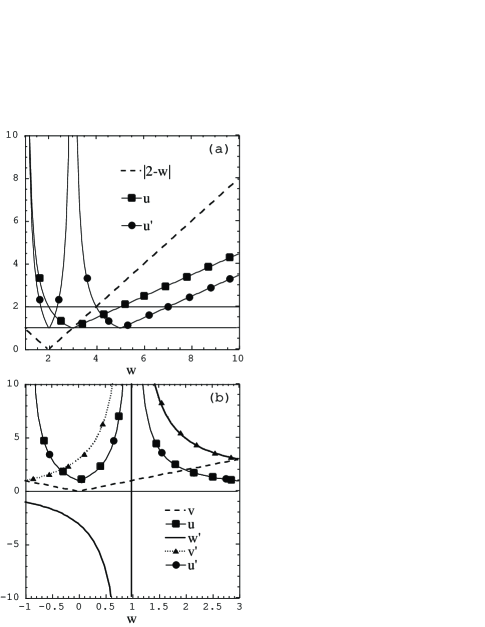
FIG. 1.: Relations between $w$, $w^{\prime}$, $u$, and $u^{\prime}$. (a) Curvature bounce: Initially, $w>1$ so that $v=w$. The dashed line shows $v^{\prime}=|w^{\prime}|=|2-w|$. Table II is used to compute $u$ for $v>1$ and $u^{\prime}$ for $0\leq v^{\prime}$. The horizontal lines show $1\leq u,u^{\prime}\leq 2$. (b) Twist bounce: Initially, $-1\leq w\leq 3$. The corresponding $u$, $v$, $w^{\prime}$, $u^{\prime}$, and $v^{\prime}$ are shown. Note that the curves for $u$ and $u^{\prime}=u$ are superposed. Table II is used to compute $u$ from $v$.

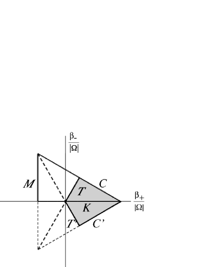
FIG. 2.: Fig. 2. The local MSS in the $\beta_{\pm}/|\Omega|$ plane. The triangle represents the Bianchi IX MSS potential. Scaling the anisotropy variables $\beta_{\pm}$ by the logarithmic volume $|\Omega|$ ($\Omega\to-\infty$ is the singularity), keeps the bounce locations fixed. The Gowdy models begin generically with the walls $C$ and $C^{\prime}$ which disappear as the spacetime becomes AVTD. In magnetic Gowdy, a third curvature-like wall $M$ is created by the magnetic field. In $T^{2}$ symmetric models, a centrifugal wall $T$ closes off the potential. Here the kinetic “wall” is understood to map $C^{\prime}$ onto $C$ so that the dynamics is confined to the shaded region.

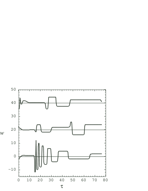
FIG. 3.: Fig. 3. Typical behavior of $w(\tau)$ at representative values of $\theta$. The upper points are offset by 20 and 40 respectively for display convenience. The flat regions characterize the Kasner epochs.

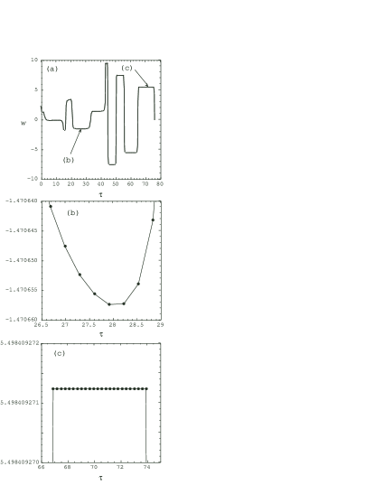
FIG. 4.: Onset and recurrence of the KEA, as monitored by $w$. (a) $w(\tau,\theta_{0})$ for fixed $\theta_{0}$. Flat regions indicate KEA. (b) and (c) Detailed closeups of $w(\tau,\theta_{0})$ at early (b) and later (c) times. At the later time, $w$ is flatter during the Kasner epoch.

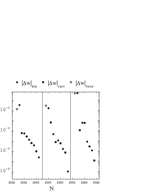
FIG. 5.: Typical behavior and accuracy of the bounce laws at three adjacent spatial points. Each point represents the smallest difference between a predicted and measured value of $w$ using all of the bounce rules. This shows that each sequence starts with a twist bounce and is followed by alternating kinetic and curvature bounces. As the simulation evolves, the accuracy of the bounce law prediction improves. The data were obtained by measuring $w$ for all bounces over a symmetric region (of length $\pi$) in the simulations. The bounces are numbered consecutively ($N$) following bounces at increasing $\tau$ at a given point and then moving to the sequence of bounces at the next point. The vertical lines divide the bounces at a given spatial point from those at the next point.

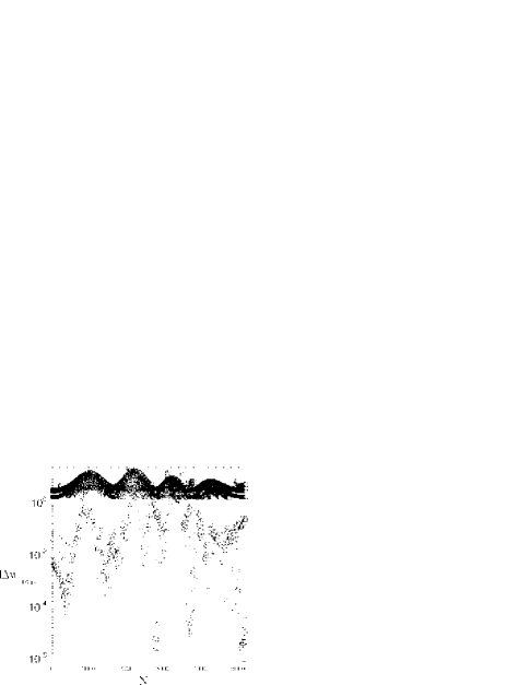
FIG. 6.: Twist bounces identified by the difference between the measured and predicted values of $w$. All bounces at all spatial points in the considered interval had their preceding and subsequent values of $w$ measured and then computed according to the twist bounce rule. Where the difference between the measured and predicted values are large, it means that the bounce was not a twist bounce. The twist bounces early in the simulation agree with the bounce rule with rather low accuracy because the KEA is not yet completely valid. The highest accuracy agreement with predictions indicates second twist bounces later in the simulation. Clustering of the more accurate twist bounces just indicates that similar behavior is occurring at nearby spatial points.

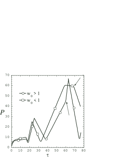
FIG. 7.: Behavior of $P$ at twist bounces. Since in a Kasner epoch, $\partial_{\tau}P=w$, the piecewise constant $w$ implies a piecewise linear $P$. The twist bounces are indicated by the arrows. If $w_{0}>1$, then $w^{\prime}>3$ and the next bounce will be a curvature bounce. If $w_{0}<1$, then $w^{\prime}<-1$ and the next bounce is kinetic.

FIG. 8.: Combined curvature and twist bounces. This graph is generated as in Fig. 6 but using the rule for combined bounces. The actual combined bounces have $|\Delta w|\approx 10^{-6}$.

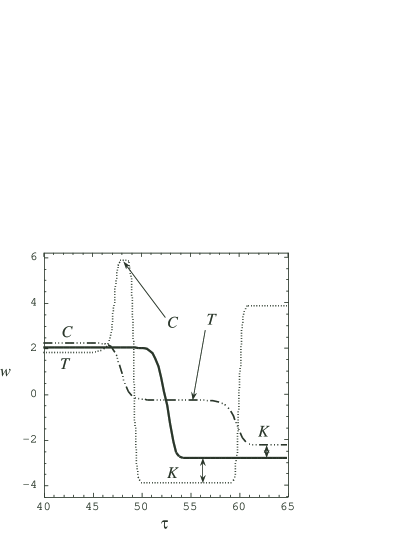
FIG. 9.: Structure of a combined bounce. The combined bounce’s $w(\tau)$ at $\theta_{0}$ is shown as a solid line. The segment after the bounce has $w<-1$ so a kinetic bounce will follow; $w(\tau)$ for a point with $\theta$ slightly less than $\theta_{0}$ is shown with the dotted line. Here the final pre-kinetic bounce segment ($K$) is preceded by pre-twist ($T$) and pre-curvature ($C$) segments. The dot-dashed line shows $w(\tau)$ for $\theta$ slightly greater than $\theta_{0}$. Here first a pre-curvature bounce and then a pre-twist bounce segment precedes the final pre-kinetic bounce segment.

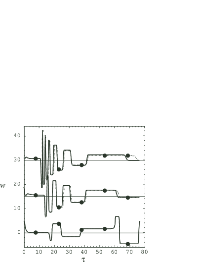
FIG. 10.: Spatial resolution dependence. The evolution (for $w(\theta,\tau)$) is shown at three representative values of $\theta$ (offset by 15 and 30 respectively) for 1024 (solid line) and 2048 (dotted line with circles) spatial grid points. The dependence on spatial resolution increases with the value of $|w|$ which follows the initial twist bounce.

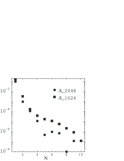
FIG. 11.: $|\Delta w|$ for a sequence of bounces at the same value of $\theta$ for different spatial resolutions. The difference between the measured and predicted values of $w$ is shown.

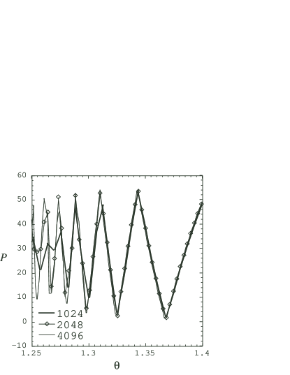
FIG. 12.: Resolution dependence of waveforms. As has been noted in the evolution of $U(1)$ symmetric cosmologies [10], narrowing spiky features [15] cause the simulations to yield resolution dependent results where the functions are not smooth. The choice of initial data made here yields an especially spiky waveform for $P$. A representative portion is shown.

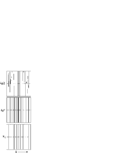
FIG. 13.: Exceptional points. Exceptional points with $\partial_{\theta}Q=0$ and $\partial_{\theta}P=0$ are associated with the peaks in $P$ while $\pi_{Q}=0$ causes apparent discontinuities in $Q$ [15, 13]. Zero crossings of all three functions are shown at a late $\tau$ value for a portion of the $\theta$-axis.

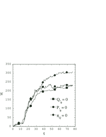
FIG. 14.: The number of exceptional points vs $\tau$. The growth in the number of exceptional points vs $\tau$ is shown. While $N$ appears to level off, this could just reflect the exponential increase of Kasner epoch duration characteristic of mixmaster dynamics. $N(\tau)$ is not a power law.

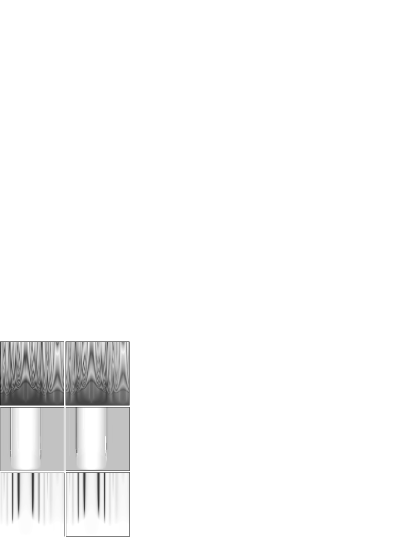
FIG. 15.: $P(\theta,\tau)$ (top), $Q(\theta,\tau)$ (middle), and $\lambda(\theta,\tau)$ (bottom) are shown for the full simulation (with arbitrary scales for their values). The left hand column uses 1024 and the right 2048 spatial grid points. In each frame, the horizontal axis is $-\pi/5\leq\theta\leq 9\pi/5$ and the vertical axis $0\leq\tau\leq 76$.

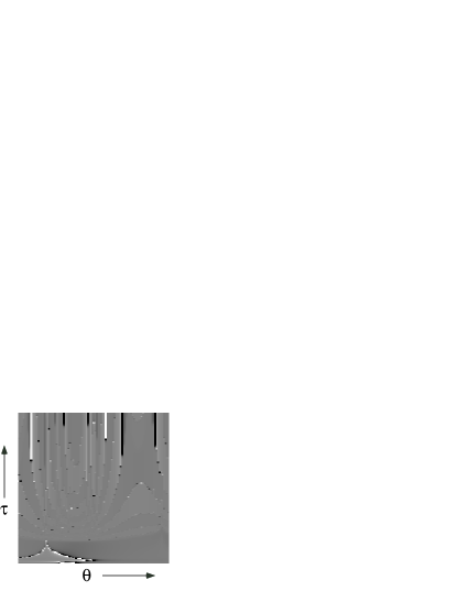
FIG. 16.: Limits on the simulation. The plot shows $w^{\prime}(\theta,\tau)$ computed from the simulations $w(\theta,\tau)$ using the twist bounce rule. The scale is set so that values $>100$ ( $<-100$) appear white (black). The white and black lines which extend to the end of the simulation indicate $\theta$-values which are destined to have dangerously large values of $w$ after the next twist bounce. Only a portion of the $\theta$ axis is shown.

REFERENCES

- [1] C. W. Misner, Phys. Rev. Lett. 22, 1071 (1969).
- [2] V. A. Belinskii, I. M. Khalatnikov, and E. M. Lifshitz, Adv. Phys. 19, 525 (1970).
- [3] E. Kasner, . J. Math. 43, 217 (1921).
- [4] A. Harvey, Gen. Relativ. Gravit. 22, 1433 (1990).
- [5] H. Ringström, Ann. Inst. Henri Poincaré (to be published), gr-qc/0006035.
- [6] V. A. Belinskii, I. M. Khalatnikov, and E. M. Lifshitz, Adv. Phys. 31, 639 (1982).
- [7] J. Isenberg, and V. Moncrief, unpublished.
- [8] M. Weaver, J. Isenberg and B. K. Berger, Phys. Rev. Lett. 80, 2984 (1998).
- [9] B. Grubišić and V. Moncrief, Phys. Rev. D 47, 2371 (1993).
- [10] B. K. Berger and V. Moncrief, Phys. Rev. D 58, 064023 (1998).
- [11] R.H. Gowdy, Phys. Rev. Lett. 27, 826 (1971).
- [12] B. K. Berger, J. Isenberg, and M. Weaver, unpublished.
- [13] B. K. Berger and D. Garfinkle, Phys. Rev. D 57, 4767 (1998).
- [14] B. K. Berger, D. Garfinkle and V. Moncrief,in Internal Structure of Black Holes and Spacetime Singularities, edited by L. M. Burko, A. Ori (Institute of Physics, Bristol, 1998), pp 441 457, gr-qc/9709073.
- [15] B. K. Berger and V. Moncrief, Phys. Rev. D 48, 4676 (1993).
- [16] J. Isenberg and V. Moncrief, Ann. Phys. (N. Y.) 199, 84 (1990).
- [17] S. Kichenassamy and A. D. Rendall, Class. Quantum Grav. 15, 1339 (1998).
- [18] A. D. Rendall, Class. Quantum Grav. 17, 3305 (2000).
- [19] A. D. Rendall and M. Weaver, “Manufacture of Gowdy spacetimes with spikes,” gr-qc/0103102.
- [20] D. Eardley, E. Liang, and R. Sachs, J. Math. Phys. 13, 99 (1972).
- [21] B. K. Berger, J. Isenberg, P. T. Chruściel, and V. Moncrief, Ann. Phys. (N. Y.) 260, 117 (1997).
- [22] P. T. Chruściel, Ann. Phys. (N. Y.) 202, 100 (1990).
- [23] S. D. Hern, Numerical Relativity and Inhomogeneous Cosmologies, Ph.D. Thesis, Cambridge University, 1999, gr-qc/0004036.
- [24] D. Garfinkle, Phys. Rev. D 60, 104010 (1999).
- [25] C. G. Hewitt and J. Wainwright, Class. Quantum Grav. 7, 2295 (1990).
- [26] J. Isenberg and S. Kichenassamy, J. Math. Phys. 40, 340 (1999).
- [27] B. K. Berger, D. Garfinkle, J. Isenberg, V. Moncrief, and M. Weaver, Mod. Phys. Lett. A13, 1565 (1998).
- [28] M. P. Ryan, Jr., Hamiltonian Cosmology, (Springer-Verlag, Heidelberg, 1972).
- [29] R. T. Jantzen, in Gamov Cosmology, edited by R. Ruffini and F. Melchiorri (North-Holland, Amsterdam, 1987), pp. 61–147, gr-qc/0102035.
- [30] C. G. Hewitt, R. Bridson, and J. Wainwright, Gen. Relativ. Gravit. 33, 65 (1990).
- [31] B. K. Berger and V. Moncrief, Phys. Rev. D 62, 123501 (2000).
- [32] S. Teukolsky, Phys. Rev. D 61, 087501 (2000).
- [33] B.K. Berger, Z. Belanger, M. Dorr, X. Garaizar, unpublished. See http://www.aps.org/meet/APR01/baps/abs/ S280006.html.
- [34] W.H. Press et al, Numerical Recipes: the Art of Scientific Computing (2nd edition), (Cambridge University, Cambridge, 1971).
- [35] B.K. Berger et al, unpublished.
- [36] M. Weaver, Asymptotic Behavior of Solutions to Einstein’s Equation, Ph.D. Thesis, University of Oregon, 1999.
- [37] B. K. Berger, D. Garfinkle, and E. Strasser, Class. Quantum Grav. 14, L29 (1997).
- [38] T. Kato, Theory for Linear Operators (Springer, Berlin, 1966).