Equation of state for a classical gas of BPS black holes

Abstract

A point particle treatment to the statistical mechanics of BPS black holes in Einstein-Maxwell-dilaton theory is developed. Because of the absence of the static potential, the canonical partition function for $N$ BPS black holes can be expressed by the volume of the moduli space for them. We estimate the equation of state for a classical gas of BPS black holes by Padé approximation and find that the result agrees with the one obtained by the mean-field approximation.

I Introduction

The thermodynamics of self-gravitating system has some importance in the context of cosmology. The long-range nature of gravity gives rise to the breakdown of the conventional description of statistical properties, such as the additivity of the free energy or other ‘extensive’ thermodynamical quantities. While the statistical treatment of non-equilibrium systems has recently been developed, the existence of the long range force seems essential for explaining the formation of the peculiar local structure in the system.

Recently, de Vega and Sánchez studied the statistical mechanics of the self-gravitating particle gas[1]. They showed that the ‘thermodynamic limit’ must be taken as $N\rightarrow\infty$ with $N/{\cal V}^{1/3}$ fixed in three dimensions, where $N$ is the number of particles and ${\cal V}$ is the volume of the system. This treatment is required by the long-range nature of gravity, because there is no ad hoc cut-off scale.

On the other hand, two of the present authors have studied the statistical mechanics of the well-separated charged particles in Einstein-Maxwell-scalar theory[2]. The system was found to be unstable in general, though there exists a critical case in which the static forces are cancelled each other.

In general relativity, the critical case was investigated and exact static solutions which describe multi-black hole systems have been obtained [3, 4, 5, 6]. In such a case, the attractive forces (the gravitational and scalar-mediated forces) and the repulsive forces (the electrostatic force) between black holes are exactly cancelled in the static limit. In this case, the energy of the system was calculated for small velocities but for small distances between the black holes[7, 8, 9, 10, 11, 12].

In this paper, we investigate the multi-black hole system by adopting the technique of de Vega and Sánchez[1]. Note that a mass-charge relation is satisfied for each individual black hole. Such extreme black holes, or so-called BPS black holes , often appear in string theories. Besides being of theoretical (academic, methodological) interest, the study on the thermodynamical aspects of them may be applied to the scenario of ‘string cosmology’.

II ‘BPS black holes’ in slow motion

We consider ‘BPS black holes’ in $(d+1)$ dimensional Einstein-Maxwell-dilaton theory, which is governed by the action

$$S = \int\!\!d^{d+1}x\,\frac{\sqrt{-g}}{16\pi G}\>\Bigl{[}\,R-\frac{4}{d-1}\nabla_{\mu}\phi\nabla^{\mu}\phi-e^{-\frac{4a}{d-1}\phi}F_{\mu\nu}F^{\mu\nu}\Bigl{]}\,.$$ (1)

Here $R$ is the scalar curvature and $F_{\mu\nu}=\partial_{\mu}A_{\nu}-\partial_{\nu}A_{\mu}$ ($\mu,\nu=0,1,\dots,d$), while $\phi$ is a dilaton field and $a$ is a coupling constant. $G$ denotes the $(d+1)$ dimensional Newton’s constant. We set $c=1$.

This theory admits static multi-centered solutions whose metric and field configurations are given by[6]

$$ds^{2} = -V^{-\frac{2(d-2)}{d-2+a^{2}}}dt^{2}+V^{\frac{2}{d-2+a^{2}}}d\mathchoice{{\hbox{\boldmath$\displaystyle x$}}}{{\hbox{\boldmath$\textstyle x$}}}{{\hbox{\boldmath$\scriptstyle x$}}}{{\hbox{\boldmath$\scriptscriptstyle x$}}}^{2}\,,$$ (2)

$$e^{-\frac{4a}{d-1}\phi} = V^{\frac{2a^{2}}{d-2+a^{2}}}\,,$$ (3)

$$A_{0}(\mathchoice{{\hbox{\boldmath$\displaystyle x$}}}{{\hbox{\boldmath$\textstyle x$}}}{{\hbox{\boldmath$\scriptstyle x$}}}{{\hbox{\boldmath$\scriptscriptstyle x$}}}) = \sqrt{\frac{d-1}{2(d-2+a^{2})}}\Bigl{(}1-\frac{1}{V}\Bigr{)}\,,$$ (4)

$$A_{i}(\mathchoice{{\hbox{\boldmath$\displaystyle x$}}}{{\hbox{\boldmath$\textstyle x$}}}{{\hbox{\boldmath$\scriptstyle x$}}}{{\hbox{\boldmath$\scriptscriptstyle x$}}}) = 0\qquad\qquad(i=1,\dots,d)\,,$$ (5)

in terms of a harmonic function

$$V(\mathchoice{{\hbox{\boldmath$\displaystyle x$}}}{{\hbox{\boldmath$\textstyle x$}}}{{\hbox{\boldmath$\scriptstyle x$}}}{{\hbox{\boldmath$\scriptscriptstyle x$}}})=1+\frac{2(d-2+a^{2})}{(d-1)(d-2)}\frac{4\pi}{A_{d-1}}\,G\sum_{a}~{}\frac{m_{a}}{|\mathchoice{{\hbox{\boldmath$\displaystyle r$}}}{{\hbox{\boldmath$\textstyle r$}}}{{\hbox{\boldmath$\scriptstyle r$}}}{{\hbox{\boldmath$\scriptscriptstyle r$}}}_{a}|^{d-2}}\,,$$ (6)

where $\mathchoice{{\hbox{\boldmath$\displaystyle r$}}}{{\hbox{\boldmath$\textstyle r$}}}{{\hbox{\boldmath$\scriptstyle r$}}}{{\hbox{\boldmath$\scriptscriptstyle r$}}}_{a}=\mathchoice{{\hbox{\boldmath$\displaystyle x$}}}{{\hbox{\boldmath$\textstyle x$}}}{{\hbox{\boldmath$\scriptstyle x$}}}{{\hbox{\boldmath$\scriptscriptstyle x$}}}-\mathchoice{{\hbox{\boldmath$\displaystyle x$}}}{{\hbox{\boldmath$\textstyle x$}}}{{\hbox{\boldmath$\scriptstyle x$}}}{{\hbox{\boldmath$\scriptscriptstyle x$}}}_{a}$, $\mathchoice{{\hbox{\boldmath$\displaystyle x$}}}{{\hbox{\boldmath$\textstyle x$}}}{{\hbox{\boldmath$\scriptstyle x$}}}{{\hbox{\boldmath$\scriptscriptstyle x$}}}_{a}$ is the position vector of ‘point particle’ $a$ and the labels of ‘particles’ $a,b,\dots$ run over $1,\dots,N$. $A_{d-1}\equiv 2\pi^{d/2}/\Gamma(d/2)$ is the volume of a unit $d-1$ sphere.

The static point sources corresponding to the ‘particles’ can be described by the action

$$I=\,-\sum_{a}\int\!\!ds_{a}\>\Bigl{[}m_{a}\,e^{\frac{2a}{d-1}\phi}+e_{a}A_{\mu}\frac{dx^{\mu}}{ds_{a}}\Bigr{]}\,,$$ (7)

with the relation

$$\frac{e_{a}}{m_{a}}=\sqrt{\frac{2(d-2+a^{2})}{d-1}}\,.$$ (8)

This relation is just the extremity condition for spherically symmetric black holes in the Einstein-Maxwell-dilaton theory[25, 26]. Thus the solution can be viewed as the one for an ‘$N$ BPS black hole’ system, where the electric force is cancelled by the forces mediated by the graviton and the dilaton.

While there is no static force between the ‘black holes’, a velocity dependent force arises if one gives them small velocities $\mathchoice{{\hbox{\boldmath$\displaystyle v$}}}{{\hbox{\boldmath$\textstyle v$}}}{{\hbox{\boldmath$\scriptstyle v$}}}{{\hbox{\boldmath$\scriptscriptstyle v$}}}_{a}$. Many authors calculated the effective theory to $O(v^{2})$ for various types of ‘black holes’. One finds the energy of the ‘BPS black holes’ in the Einstein-Maxwell-dilaton theory [12]

$$H=\sum_{a}\sum_{b}v^{ak}v^{b\ell}(\delta^{i}_{k}\delta^{j}_{\ell}+\delta_{k\ell}\delta^{ij}-\delta^{j}_{k}\delta^{i}_{\ell})\partial_{ai}\partial_{bj}L\,,$$ (9)

where

$$L=-\frac{1}{32\pi G}\int d^{d}\mathchoice{{\hbox{\boldmath$\displaystyle x$}}}{{\hbox{\boldmath$\textstyle x$}}}{{\hbox{\boldmath$\scriptstyle x$}}}{{\hbox{\boldmath$\scriptscriptstyle x$}}}~{}V^{\frac{2(d-1)}{d-2+a^{2}}}(\mathchoice{{\hbox{\boldmath$\displaystyle x$}}}{{\hbox{\boldmath$\textstyle x$}}}{{\hbox{\boldmath$\scriptstyle x$}}}{{\hbox{\boldmath$\scriptscriptstyle x$}}})\,,$$ (10)

with $V$ given by (6) and the spatial indices $i,j,\dots$ run over $1,\dots,d$.

III The canonical partition function

The canonical partition function for $N$ identical particles at temperature $T$ in $d$ spatial dimensions is

$$Z_{N}=\frac{1}{N!}\frac{1}{h^{Nd}}\int[{\rm dq}][{\rm dp}]\exp\left(-\beta H\right)\,,$$ (11)

where $[{\rm dp}]=\prod_{a=1}^{N}d^{d}\mathchoice{{\hbox{\boldmath$\displaystyle p$}}}{{\hbox{\boldmath$\textstyle p$}}}{{\hbox{\boldmath$\scriptstyle p$}}}{{\hbox{\boldmath$\scriptscriptstyle p$}}}_{a}$ and $[{\rm dq}]=\prod_{a=1}^{N}d^{d}\mathchoice{{\hbox{\boldmath$\displaystyle x$}}}{{\hbox{\boldmath$\textstyle x$}}}{{\hbox{\boldmath$\scriptstyle x$}}}{{\hbox{\boldmath$\scriptscriptstyle x$}}}_{a}$. $\beta=1/T$, where $h$ is Planck’s constant while Boltzmann’s constant is set to be unity.

Because there is no static forces, the Hamiltonian $H$ for the system of $N$ ‘BPS black holes’ can be written as

$$H=\frac{1}{2}\sum_{A}\sum_{B}~{}v^{A}{\cal G}_{AB}v^{B}=\frac{1}{2}\mathchoice{{\hbox{\boldmath$\displaystyle v$}}}{{\hbox{\boldmath$\textstyle v$}}}{{\hbox{\boldmath$\scriptstyle v$}}}{{\hbox{\boldmath$\scriptscriptstyle v$}}}^{T}\mathchoice{{\hbox{\boldmath$\displaystyle\cal G$}}}{{\hbox{\boldmath$\textstyle\cal G$}}}{{\hbox{\boldmath$\scriptstyle\cal G$}}}{{\hbox{\boldmath$\scriptscriptstyle\cal G$}}}\mathchoice{{\hbox{\boldmath$\displaystyle v$}}}{{\hbox{\boldmath$\textstyle v$}}}{{\hbox{\boldmath$\scriptstyle v$}}}{{\hbox{\boldmath$\scriptscriptstyle v$}}}\,,$$ (12)

where the label $\{A\}=\{(ai)\}$ denotes the combination of the label of the particle and the spatial index.

The canonical momentum can be found as

$$p_{A}=\frac{\partial H}{\partial v^{A}}=\sum_{B}{\cal G}_{AB}~{}v^{B}=(\mathchoice{{\hbox{\boldmath$\displaystyle\cal G$}}}{{\hbox{\boldmath$\textstyle\cal G$}}}{{\hbox{\boldmath$\scriptstyle\cal G$}}}{{\hbox{\boldmath$\scriptscriptstyle\cal G$}}}\mathchoice{{\hbox{\boldmath$\displaystyle v$}}}{{\hbox{\boldmath$\textstyle v$}}}{{\hbox{\boldmath$\scriptstyle v$}}}{{\hbox{\boldmath$\scriptscriptstyle v$}}})_{A}\,,$$ (13)

and then the Hamiltonian is reexpressed as

$$H=\frac{1}{2}\sum_{A}\sum_{B}~{}p_{A}{\cal G}^{AB}p_{B}=\frac{1}{2}\mathchoice{{\hbox{\boldmath$\displaystyle p$}}}{{\hbox{\boldmath$\textstyle p$}}}{{\hbox{\boldmath$\scriptstyle p$}}}{{\hbox{\boldmath$\scriptscriptstyle p$}}}^{T}\mathchoice{{\hbox{\boldmath$\displaystyle\cal G$}}}{{\hbox{\boldmath$\textstyle\cal G$}}}{{\hbox{\boldmath$\scriptstyle\cal G$}}}{{\hbox{\boldmath$\scriptscriptstyle\cal G$}}}^{-1}\mathchoice{{\hbox{\boldmath$\displaystyle p$}}}{{\hbox{\boldmath$\textstyle p$}}}{{\hbox{\boldmath$\scriptstyle p$}}}{{\hbox{\boldmath$\scriptscriptstyle p$}}}\,.$$ (14)

Thus the partition function becomes

$$Z_{N}=\frac{1}{N!}\left(\frac{2\pi}{\beta h^{2}}\right)^{\frac{Nd}{2}}\int[{\rm dq}]\sqrt{\det\mathchoice{{\hbox{\boldmath$\displaystyle\cal G$}}}{{\hbox{\boldmath$\textstyle\cal G$}}}{{\hbox{\boldmath$\scriptstyle\cal G$}}}{{\hbox{\boldmath$\scriptscriptstyle\cal G$}}}}\,.$$ (15)

If we define

$$L^{\prime}=-\frac{1}{32\pi G}\int d^{d}\mathchoice{{\hbox{\boldmath$\displaystyle x$}}}{{\hbox{\boldmath$\textstyle x$}}}{{\hbox{\boldmath$\scriptstyle x$}}}{{\hbox{\boldmath$\scriptscriptstyle x$}}}\left[V^{\frac{2(d-1)}{d-2+a^{2}}}(\mathchoice{{\hbox{\boldmath$\displaystyle x$}}}{{\hbox{\boldmath$\textstyle x$}}}{{\hbox{\boldmath$\scriptstyle x$}}}{{\hbox{\boldmath$\scriptscriptstyle x$}}})-1-\frac{4}{d-2}\frac{4\pi}{A_{d-1}}\,Gm\sum_{c}~{}\frac{1}{|\mathchoice{{\hbox{\boldmath$\displaystyle r$}}}{{\hbox{\boldmath$\textstyle r$}}}{{\hbox{\boldmath$\scriptstyle r$}}}{{\hbox{\boldmath$\scriptscriptstyle r$}}}_{c}|^{d-2}}\right]\,,$$ (16)

with

$$V(\mathchoice{{\hbox{\boldmath$\displaystyle x$}}}{{\hbox{\boldmath$\textstyle x$}}}{{\hbox{\boldmath$\scriptstyle x$}}}{{\hbox{\boldmath$\scriptscriptstyle x$}}})=1+\frac{2(d-2+a^{2})}{(d-1)(d-2)}\frac{4\pi}{A_{d-1}}\,Gm\sum_{a}~{}\frac{1}{|\mathchoice{{\hbox{\boldmath$\displaystyle r$}}}{{\hbox{\boldmath$\textstyle r$}}}{{\hbox{\boldmath$\scriptstyle r$}}}{{\hbox{\boldmath$\scriptscriptstyle r$}}}_{a}|^{d-2}}\,,$$ (17)

the Hamiltonian for $N$ ‘BPS black holes’ with a common mass $m$ can be rewritten as

$$H=\frac{1}{2}m\sum_{a}\mathchoice{{\hbox{\boldmath$\displaystyle v$}}}{{\hbox{\boldmath$\textstyle v$}}}{{\hbox{\boldmath$\scriptstyle v$}}}{{\hbox{\boldmath$\scriptscriptstyle v$}}}_{a}^{2}+\sum_{a}\sum_{b}v^{ak}v^{b\ell}(\delta_{k\ell}\delta^{ij}+\delta^{i}_{k}\delta^{j}_{\ell}-\delta^{j}_{k}\delta^{i}_{\ell})\partial_{ai}\partial_{bj}L^{\prime}\,.$$ (18)

Then we may use

$${\cal G}_{(ak)(b\ell)}=m\left[\delta_{ab}\delta_{k\ell}+\frac{2}{m}(\delta_{k\ell}\delta^{ij}+\delta^{i}_{k}\delta^{j}_{\ell}-\delta^{j}_{k}\delta^{i}_{\ell})\partial_{ai}\partial_{bj}L^{\prime}\right]\equiv m~{}g_{(ak)(b\ell)}\,,$$ (19)

and obtain the expression for the partition function

$$Z_{N}=\frac{1}{N!}\left(\frac{2\pi m}{\beta h^{2}}\right)^{\frac{Nd}{2}}\int[{\rm dq}]\sqrt{\det\mathchoice{{\hbox{\boldmath$\displaystyle g$}}}{{\hbox{\boldmath$\textstyle g$}}}{{\hbox{\boldmath$\scriptstyle g$}}}{{\hbox{\boldmath$\scriptscriptstyle g$}}}}\equiv\frac{1}{N!}\left(\frac{2\pi m}{\beta h^{2}}\right)^{\frac{Nd}{2}}Q\,,$$ (20)

which is proportial to the volume of the moduli space $Q$. This feature is the same as that of point-particle systems in two (spatial) dimensions[27, 28], in which there is no static force either.

In the present system, the free energy $F$ is expressed as

$$F=-T\ln Z=NT\ln N-NT-\frac{d}{2}NT\ln\frac{2\pi m}{\beta h^{2}}-NT\ln{\cal V}-T\ln\frac{Q}{{\cal V}^{N}}\,.$$ (21)

Therefore the internal energy $E$ is obtained as

$$\frac{E}{N}=\frac{1}{N}\frac{\partial(\beta F)}{\partial\beta}=\frac{d}{2}T\,,$$ (22)

which is the same as that of an ideal gas.

IV The perturbative approach

To obtain the equation of state, we have to evaluate the volume of the moduli space $Q$.

First, we try to obtain the volume of the moduli space perturbatively. One can rewrite this as

$$Q \equiv \int[{\rm dq}]\sqrt{\det\mathchoice{{\hbox{\boldmath$\displaystyle g$}}}{{\hbox{\boldmath$\textstyle g$}}}{{\hbox{\boldmath$\scriptstyle g$}}}{{\hbox{\boldmath$\scriptscriptstyle g$}}}}=\int[{\rm dq}]\exp\left(\frac{1}{2}\mbox{Tr}\ln\mathchoice{{\hbox{\boldmath$\displaystyle g$}}}{{\hbox{\boldmath$\textstyle g$}}}{{\hbox{\boldmath$\scriptstyle g$}}}{{\hbox{\boldmath$\scriptscriptstyle g$}}}\right)$$ (23)

$$= \int[{\rm dq}]\exp\left[\frac{1}{2}\mbox{Tr}(\mathchoice{{\hbox{\boldmath$\displaystyle u$}}}{{\hbox{\boldmath$\textstyle u$}}}{{\hbox{\boldmath$\scriptstyle u$}}}{{\hbox{\boldmath$\scriptscriptstyle u$}}}-\frac{1}{2}\mathchoice{{\hbox{\boldmath$\displaystyle u$}}}{{\hbox{\boldmath$\textstyle u$}}}{{\hbox{\boldmath$\scriptstyle u$}}}{{\hbox{\boldmath$\scriptscriptstyle u$}}}^{2}+\cdots)\right]$$ (24)

$$= \int[{\rm dq}]\left[1+\frac{1}{2}\mbox{Tr}\mathchoice{{\hbox{\boldmath$\displaystyle u$}}}{{\hbox{\boldmath$\textstyle u$}}}{{\hbox{\boldmath$\scriptstyle u$}}}{{\hbox{\boldmath$\scriptscriptstyle u$}}}-\frac{1}{4}\mbox{Tr}\mathchoice{{\hbox{\boldmath$\displaystyle u$}}}{{\hbox{\boldmath$\textstyle u$}}}{{\hbox{\boldmath$\scriptstyle u$}}}{{\hbox{\boldmath$\scriptscriptstyle u$}}}^{2}+\frac{1}{8}(\mbox{Tr}\mathchoice{{\hbox{\boldmath$\displaystyle u$}}}{{\hbox{\boldmath$\textstyle u$}}}{{\hbox{\boldmath$\scriptstyle u$}}}{{\hbox{\boldmath$\scriptscriptstyle u$}}})^{2}+\cdots\right]\,,$$ (25)

where

$$u_{(ak)(b\ell)}=\frac{2}{m}(\delta_{k\ell}\delta^{ij}+\delta^{i}_{k}\delta^{j}_{\ell}-\delta^{j}_{k}\delta^{i}_{\ell})\partial_{ai}\partial_{bj}L^{\prime}\,.$$ (26)

The term including the trace takes the form:

$$\mbox{Tr}\mathchoice{{\hbox{\boldmath$\displaystyle u$}}}{{\hbox{\boldmath$\textstyle u$}}}{{\hbox{\boldmath$\scriptstyle u$}}}{{\hbox{\boldmath$\scriptscriptstyle u$}}}=\frac{2d}{m}\sum_{a}\partial_{ai}\partial_{ai}L^{\prime}\,,$$ (27)

and

$$\mbox{Tr}\mathchoice{{\hbox{\boldmath$\displaystyle u$}}}{{\hbox{\boldmath$\textstyle u$}}}{{\hbox{\boldmath$\scriptstyle u$}}}{{\hbox{\boldmath$\scriptscriptstyle u$}}}^{2}=\frac{4}{m^{2}}\left[d~{}\delta^{ij}\delta^{i^{\prime}j^{\prime}}+2(\delta^{ii^{\prime}}\delta^{jj^{\prime}}-\delta^{ij^{\prime}}\delta^{ji^{\prime}})\right]\sum_{a}\sum_{b}\partial_{ai}\partial_{bj}L^{\prime}\partial_{ai^{\prime}}\partial_{bj^{\prime}}L^{\prime}\,.$$ (28)

To obtain the leading and next-to-leading contributions for a small $m$, we expand $L^{\prime}$ as

$$L^{\prime}=-\frac{1}{32\pi}\int d^{d}\mathchoice{{\hbox{\boldmath$\displaystyle x$}}}{{\hbox{\boldmath$\textstyle x$}}}{{\hbox{\boldmath$\scriptstyle x$}}}{{\hbox{\boldmath$\scriptscriptstyle x$}}} \left[\frac{1}{2}\left(\frac{4}{d-2}\frac{4\pi}{A_{d-1}}\right)^{2}\frac{d-a^{2}}{2(d-1)}Gm^{2}\sum_{c}\sum_{d}\frac{1}{|\mathchoice{{\hbox{\boldmath$\displaystyle r$}}}{{\hbox{\boldmath$\textstyle r$}}}{{\hbox{\boldmath$\scriptstyle r$}}}{{\hbox{\boldmath$\scriptscriptstyle r$}}}_{c}|^{d-2}}\frac{1}{|\mathchoice{{\hbox{\boldmath$\displaystyle r$}}}{{\hbox{\boldmath$\textstyle r$}}}{{\hbox{\boldmath$\scriptstyle r$}}}{{\hbox{\boldmath$\scriptscriptstyle r$}}}_{d}|^{d-2}}\right.$$ (31)

$$\left.+\frac{1}{6}\left(\frac{4}{d-2}\frac{4\pi}{A_{d-1}}\right)^{3}\frac{d-a^{2}}{2(d-1)}\frac{1-a^{2}}{d-1}G^{2}m^{3}\sum_{c}\sum_{d}\sum_{e}\frac{1}{|\mathchoice{{\hbox{\boldmath$\displaystyle r$}}}{{\hbox{\boldmath$\textstyle r$}}}{{\hbox{\boldmath$\scriptstyle r$}}}{{\hbox{\boldmath$\scriptscriptstyle r$}}}_{c}|^{d-2}}\frac{1}{|\mathchoice{{\hbox{\boldmath$\displaystyle r$}}}{{\hbox{\boldmath$\textstyle r$}}}{{\hbox{\boldmath$\scriptstyle r$}}}{{\hbox{\boldmath$\scriptscriptstyle r$}}}_{d}|^{d-2}}\frac{1}{|\mathchoice{{\hbox{\boldmath$\displaystyle r$}}}{{\hbox{\boldmath$\textstyle r$}}}{{\hbox{\boldmath$\scriptstyle r$}}}{{\hbox{\boldmath$\scriptscriptstyle r$}}}_{e}|^{d-2}}\right]$$

$$+O(m^{4})\,.$$

Using this, the traces can be written as

Tr$$u = d\left(\frac{4}{d-2}\frac{4\pi}{A_{d-1}}\right)\frac{d-a^{2}}{2(d-1)}Gm\mathop{\sum\sum}_{a\mbox{$\,/\!\!\!\!\!=\,$}b}\frac{1}{|\mathchoice{{\hbox{\boldmath$\displaystyle x$}}}{{\hbox{\boldmath$\textstyle x$}}}{{\hbox{\boldmath$\scriptstyle x$}}}{{\hbox{\boldmath$\scriptscriptstyle x$}}}_{a}-\mathchoice{{\hbox{\boldmath$\displaystyle x$}}}{{\hbox{\boldmath$\textstyle x$}}}{{\hbox{\boldmath$\scriptstyle x$}}}{{\hbox{\boldmath$\scriptscriptstyle x$}}}_{b}|^{d-2}}$$ (35)

$$+\frac{d}{2}\left(\frac{4}{d-2}\frac{4\pi}{A_{d-1}}\right)^{2}\frac{d-a^{2}}{2(d-1)}\frac{1-a^{2}}{d-1}G^{2}m^{2}$$

$$~{}\times\left[\mathop{\sum\sum\sum}_{b\mbox{$\,/\!\!\!\!\!=\,$}a,c\mbox{$\,/\!\!\!\!\!=\,$}a}\frac{1}{|\mathchoice{{\hbox{\boldmath$\displaystyle x$}}}{{\hbox{\boldmath$\textstyle x$}}}{{\hbox{\boldmath$\scriptstyle x$}}}{{\hbox{\boldmath$\scriptscriptstyle x$}}}_{a}-\mathchoice{{\hbox{\boldmath$\displaystyle x$}}}{{\hbox{\boldmath$\textstyle x$}}}{{\hbox{\boldmath$\scriptstyle x$}}}{{\hbox{\boldmath$\scriptscriptstyle x$}}}_{b}|^{d-2}}\frac{1}{|\mathchoice{{\hbox{\boldmath$\displaystyle x$}}}{{\hbox{\boldmath$\textstyle x$}}}{{\hbox{\boldmath$\scriptstyle x$}}}{{\hbox{\boldmath$\scriptscriptstyle x$}}}_{a}-\mathchoice{{\hbox{\boldmath$\displaystyle x$}}}{{\hbox{\boldmath$\textstyle x$}}}{{\hbox{\boldmath$\scriptstyle x$}}}{{\hbox{\boldmath$\scriptscriptstyle x$}}}_{c}|^{d-2}}+\mathop{\sum\sum}_{a\mbox{$\,/\!\!\!\!\!=\,$}b}\frac{1}{|\mathchoice{{\hbox{\boldmath$\displaystyle x$}}}{{\hbox{\boldmath$\textstyle x$}}}{{\hbox{\boldmath$\scriptstyle x$}}}{{\hbox{\boldmath$\scriptscriptstyle x$}}}_{a}-\mathchoice{{\hbox{\boldmath$\displaystyle x$}}}{{\hbox{\boldmath$\textstyle x$}}}{{\hbox{\boldmath$\scriptstyle x$}}}{{\hbox{\boldmath$\scriptscriptstyle x$}}}_{b}|^{2(d-2)}}\right]$$

$$+O((Gm)^{3})\,,$$

$$\mbox{Tr}\,\mathchoice{{\hbox{\boldmath$\displaystyle u$}}}{{\hbox{\boldmath$\textstyle u$}}}{{\hbox{\boldmath$\scriptstyle u$}}}{{\hbox{\boldmath$\scriptscriptstyle u$}}}^{2} = d\left(\frac{4}{d-2}\frac{4\pi}{A_{d-1}}\right)^{2}\left(\frac{d-a^{2}}{2(d-1)}\right)^{2}G^{2}m^{2}$$ (38)

$$~{}\times\left[\mathop{\sum\sum\sum}_{b\mbox{$\,/\!\!\!\!\!=\,$}a,c\mbox{$\,/\!\!\!\!\!=\,$}a}\frac{1}{|\mathchoice{{\hbox{\boldmath$\displaystyle x$}}}{{\hbox{\boldmath$\textstyle x$}}}{{\hbox{\boldmath$\scriptstyle x$}}}{{\hbox{\boldmath$\scriptscriptstyle x$}}}_{a}-\mathchoice{{\hbox{\boldmath$\displaystyle x$}}}{{\hbox{\boldmath$\textstyle x$}}}{{\hbox{\boldmath$\scriptstyle x$}}}{{\hbox{\boldmath$\scriptscriptstyle x$}}}_{b}|^{d-2}}\frac{1}{|\mathchoice{{\hbox{\boldmath$\displaystyle x$}}}{{\hbox{\boldmath$\textstyle x$}}}{{\hbox{\boldmath$\scriptstyle x$}}}{{\hbox{\boldmath$\scriptscriptstyle x$}}}_{a}-\mathchoice{{\hbox{\boldmath$\displaystyle x$}}}{{\hbox{\boldmath$\textstyle x$}}}{{\hbox{\boldmath$\scriptstyle x$}}}{{\hbox{\boldmath$\scriptscriptstyle x$}}}_{c}|^{d-2}}+\mathop{\sum\sum}_{a\mbox{$\,/\!\!\!\!\!=\,$}b}\frac{1}{|\mathchoice{{\hbox{\boldmath$\displaystyle x$}}}{{\hbox{\boldmath$\textstyle x$}}}{{\hbox{\boldmath$\scriptstyle x$}}}{{\hbox{\boldmath$\scriptscriptstyle x$}}}_{a}-\mathchoice{{\hbox{\boldmath$\displaystyle x$}}}{{\hbox{\boldmath$\textstyle x$}}}{{\hbox{\boldmath$\scriptstyle x$}}}{{\hbox{\boldmath$\scriptscriptstyle x$}}}_{b}|^{2(d-2)}}\right]$$

$$+O((Gm)^{3})\,.$$

Then we can obtain the folowing expression for $Q$:

$$\frac{Q}{{\cal V}^{N}} = 1+\frac{d}{2}\left(\frac{4}{d-2}\frac{4\pi}{A_{d-1}}\right)\frac{d-a^{2}}{2(d-1)}\,Gm\,N(N-1)\frac{1}{{\cal V}^{2}}\int\!\!\!\int\frac{d^{d}\mathchoice{{\hbox{\boldmath$\displaystyle x$}}}{{\hbox{\boldmath$\textstyle x$}}}{{\hbox{\boldmath$\scriptstyle x$}}}{{\hbox{\boldmath$\scriptscriptstyle x$}}}_{1}d^{d}\mathchoice{{\hbox{\boldmath$\displaystyle x$}}}{{\hbox{\boldmath$\textstyle x$}}}{{\hbox{\boldmath$\scriptstyle x$}}}{{\hbox{\boldmath$\scriptscriptstyle x$}}}_{2}}{|\mathchoice{{\hbox{\boldmath$\displaystyle x$}}}{{\hbox{\boldmath$\textstyle x$}}}{{\hbox{\boldmath$\scriptstyle x$}}}{{\hbox{\boldmath$\scriptscriptstyle x$}}}_{1}-\mathchoice{{\hbox{\boldmath$\displaystyle x$}}}{{\hbox{\boldmath$\textstyle x$}}}{{\hbox{\boldmath$\scriptstyle x$}}}{{\hbox{\boldmath$\scriptscriptstyle x$}}}_{2}|^{d-2}}$$ (47)

$$-\frac{d}{4}\left(\frac{4}{d-2}\frac{4\pi}{A_{d-1}}\right)^{2}\frac{d-a^{2}}{2(d-1)}\frac{d-2+a^{2}}{2(d-1)}\,G^{2}m^{2}$$

$$~{}\times\left[N(N-1)(N-2)\frac{1}{{\cal V}^{3}}\int\!\!\!\int\!\!\!\int\frac{d^{d}\mathchoice{{\hbox{\boldmath$\displaystyle x$}}}{{\hbox{\boldmath$\textstyle x$}}}{{\hbox{\boldmath$\scriptstyle x$}}}{{\hbox{\boldmath$\scriptscriptstyle x$}}}_{1}d^{d}\mathchoice{{\hbox{\boldmath$\displaystyle x$}}}{{\hbox{\boldmath$\textstyle x$}}}{{\hbox{\boldmath$\scriptstyle x$}}}{{\hbox{\boldmath$\scriptscriptstyle x$}}}_{2}d^{d}\mathchoice{{\hbox{\boldmath$\displaystyle x$}}}{{\hbox{\boldmath$\textstyle x$}}}{{\hbox{\boldmath$\scriptstyle x$}}}{{\hbox{\boldmath$\scriptscriptstyle x$}}}_{3}}{|\mathchoice{{\hbox{\boldmath$\displaystyle x$}}}{{\hbox{\boldmath$\textstyle x$}}}{{\hbox{\boldmath$\scriptstyle x$}}}{{\hbox{\boldmath$\scriptscriptstyle x$}}}_{1}-\mathchoice{{\hbox{\boldmath$\displaystyle x$}}}{{\hbox{\boldmath$\textstyle x$}}}{{\hbox{\boldmath$\scriptstyle x$}}}{{\hbox{\boldmath$\scriptscriptstyle x$}}}_{2}|^{d-2}|\mathchoice{{\hbox{\boldmath$\displaystyle x$}}}{{\hbox{\boldmath$\textstyle x$}}}{{\hbox{\boldmath$\scriptstyle x$}}}{{\hbox{\boldmath$\scriptscriptstyle x$}}}_{1}-\mathchoice{{\hbox{\boldmath$\displaystyle x$}}}{{\hbox{\boldmath$\textstyle x$}}}{{\hbox{\boldmath$\scriptstyle x$}}}{{\hbox{\boldmath$\scriptscriptstyle x$}}}_{3}|^{d-2}}\right.$$

$$\left.\qquad+2N(N-1)\frac{1}{{\cal V}^{2}}\int\!\!\!\int\frac{d^{d}\mathchoice{{\hbox{\boldmath$\displaystyle x$}}}{{\hbox{\boldmath$\textstyle x$}}}{{\hbox{\boldmath$\scriptstyle x$}}}{{\hbox{\boldmath$\scriptscriptstyle x$}}}_{1}d^{d}\mathchoice{{\hbox{\boldmath$\displaystyle x$}}}{{\hbox{\boldmath$\textstyle x$}}}{{\hbox{\boldmath$\scriptstyle x$}}}{{\hbox{\boldmath$\scriptscriptstyle x$}}}_{2}}{|\mathchoice{{\hbox{\boldmath$\displaystyle x$}}}{{\hbox{\boldmath$\textstyle x$}}}{{\hbox{\boldmath$\scriptstyle x$}}}{{\hbox{\boldmath$\scriptscriptstyle x$}}}_{1}-\mathchoice{{\hbox{\boldmath$\displaystyle x$}}}{{\hbox{\boldmath$\textstyle x$}}}{{\hbox{\boldmath$\scriptstyle x$}}}{{\hbox{\boldmath$\scriptscriptstyle x$}}}_{2}|^{2(d-2)}}\right]$$

$$+\frac{d^{2}}{8}\left(\frac{4}{d-2}\frac{4\pi}{A_{d-1}}\right)^{2}\left(\frac{d-a^{2}}{2(d-1)}\right)^{2}G^{2}m^{2}$$

$$~{}\times\left[N(N-1)(N-2)(N-3)\left(\frac{1}{{\cal V}^{2}}\int\!\!\!\int\frac{d^{d}\mathchoice{{\hbox{\boldmath$\displaystyle x$}}}{{\hbox{\boldmath$\textstyle x$}}}{{\hbox{\boldmath$\scriptstyle x$}}}{{\hbox{\boldmath$\scriptscriptstyle x$}}}_{1}d^{d}\mathchoice{{\hbox{\boldmath$\displaystyle x$}}}{{\hbox{\boldmath$\textstyle x$}}}{{\hbox{\boldmath$\scriptstyle x$}}}{{\hbox{\boldmath$\scriptscriptstyle x$}}}_{2}}{|\mathchoice{{\hbox{\boldmath$\displaystyle x$}}}{{\hbox{\boldmath$\textstyle x$}}}{{\hbox{\boldmath$\scriptstyle x$}}}{{\hbox{\boldmath$\scriptscriptstyle x$}}}_{1}-\mathchoice{{\hbox{\boldmath$\displaystyle x$}}}{{\hbox{\boldmath$\textstyle x$}}}{{\hbox{\boldmath$\scriptstyle x$}}}{{\hbox{\boldmath$\scriptscriptstyle x$}}}_{2}|^{d-2}}\right)^{2}\right.$$

$$\qquad+4N(N-1)(N-2)\frac{1}{{\cal V}^{3}}\int\!\!\!\int\!\!\!\int\frac{d^{d}\mathchoice{{\hbox{\boldmath$\displaystyle x$}}}{{\hbox{\boldmath$\textstyle x$}}}{{\hbox{\boldmath$\scriptstyle x$}}}{{\hbox{\boldmath$\scriptscriptstyle x$}}}_{1}d^{d}\mathchoice{{\hbox{\boldmath$\displaystyle x$}}}{{\hbox{\boldmath$\textstyle x$}}}{{\hbox{\boldmath$\scriptstyle x$}}}{{\hbox{\boldmath$\scriptscriptstyle x$}}}_{2}d^{d}\mathchoice{{\hbox{\boldmath$\displaystyle x$}}}{{\hbox{\boldmath$\textstyle x$}}}{{\hbox{\boldmath$\scriptstyle x$}}}{{\hbox{\boldmath$\scriptscriptstyle x$}}}_{3}}{|\mathchoice{{\hbox{\boldmath$\displaystyle x$}}}{{\hbox{\boldmath$\textstyle x$}}}{{\hbox{\boldmath$\scriptstyle x$}}}{{\hbox{\boldmath$\scriptscriptstyle x$}}}_{1}-\mathchoice{{\hbox{\boldmath$\displaystyle x$}}}{{\hbox{\boldmath$\textstyle x$}}}{{\hbox{\boldmath$\scriptstyle x$}}}{{\hbox{\boldmath$\scriptscriptstyle x$}}}_{2}|^{d-2}|\mathchoice{{\hbox{\boldmath$\displaystyle x$}}}{{\hbox{\boldmath$\textstyle x$}}}{{\hbox{\boldmath$\scriptstyle x$}}}{{\hbox{\boldmath$\scriptscriptstyle x$}}}_{1}-\mathchoice{{\hbox{\boldmath$\displaystyle x$}}}{{\hbox{\boldmath$\textstyle x$}}}{{\hbox{\boldmath$\scriptstyle x$}}}{{\hbox{\boldmath$\scriptscriptstyle x$}}}_{3}|^{d-2}}$$

$$\left.\qquad+2N(N-1)\frac{1}{{\cal V}^{2}}\int\!\!\!\int\frac{d^{d}\mathchoice{{\hbox{\boldmath$\displaystyle x$}}}{{\hbox{\boldmath$\textstyle x$}}}{{\hbox{\boldmath$\scriptstyle x$}}}{{\hbox{\boldmath$\scriptscriptstyle x$}}}_{1}d^{d}\mathchoice{{\hbox{\boldmath$\displaystyle x$}}}{{\hbox{\boldmath$\textstyle x$}}}{{\hbox{\boldmath$\scriptstyle x$}}}{{\hbox{\boldmath$\scriptscriptstyle x$}}}_{2}}{|\mathchoice{{\hbox{\boldmath$\displaystyle x$}}}{{\hbox{\boldmath$\textstyle x$}}}{{\hbox{\boldmath$\scriptstyle x$}}}{{\hbox{\boldmath$\scriptscriptstyle x$}}}_{1}-\mathchoice{{\hbox{\boldmath$\displaystyle x$}}}{{\hbox{\boldmath$\textstyle x$}}}{{\hbox{\boldmath$\scriptstyle x$}}}{{\hbox{\boldmath$\scriptscriptstyle x$}}}_{2}|^{2(d-2)}}\right]$$

$$+O((Gm)^{3})\,,$$

where ${\cal V}=\int d^{d}\mathchoice{{\hbox{\boldmath$\displaystyle x$}}}{{\hbox{\boldmath$\textstyle x$}}}{{\hbox{\boldmath$\scriptstyle x$}}}{{\hbox{\boldmath$\scriptscriptstyle x$}}}$.

This expression includes divergent integrals and thus we must use the small cut-off length. These terms are, however, eliminated by $1/N$ factors in the $N\rightarrow\infty$ limit[1].

In the thermodynamical limit, or in the limit of large $N$, we obtain

$$\lim_{N\rightarrow\infty}\frac{1}{N}\ln\frac{Q}{{\cal V}^{N}} = \frac{d}{2}\left(\frac{4}{d-2}\frac{4\pi}{A_{d-1}}\frac{GmN}{\ell^{d-2}}\right)\frac{d-a^{2}}{2(d-1)}\frac{\ell^{d-2}}{{\cal V}^{2}}\int\!\!\!\int\frac{d^{d}\mathchoice{{\hbox{\boldmath$\displaystyle x$}}}{{\hbox{\boldmath$\textstyle x$}}}{{\hbox{\boldmath$\scriptstyle x$}}}{{\hbox{\boldmath$\scriptscriptstyle x$}}}_{1}d^{d}\mathchoice{{\hbox{\boldmath$\displaystyle x$}}}{{\hbox{\boldmath$\textstyle x$}}}{{\hbox{\boldmath$\scriptstyle x$}}}{{\hbox{\boldmath$\scriptscriptstyle x$}}}_{2}}{|\mathchoice{{\hbox{\boldmath$\displaystyle x$}}}{{\hbox{\boldmath$\textstyle x$}}}{{\hbox{\boldmath$\scriptstyle x$}}}{{\hbox{\boldmath$\scriptscriptstyle x$}}}_{1}-\mathchoice{{\hbox{\boldmath$\displaystyle x$}}}{{\hbox{\boldmath$\textstyle x$}}}{{\hbox{\boldmath$\scriptstyle x$}}}{{\hbox{\boldmath$\scriptscriptstyle x$}}}_{2}|^{d-2}}$$ (52)

$$-\frac{d^{2}}{2}\left(\frac{4}{d-2}\frac{4\pi}{A_{d-1}}\frac{GmN}{\ell^{d-2}}\right)^{2}\left(\frac{d-a^{2}}{2(d-1)}\right)^{2}\left(\frac{\ell^{d-2}}{{\cal V}^{2}}\int\!\!\!\int\frac{d^{d}\mathchoice{{\hbox{\boldmath$\displaystyle x$}}}{{\hbox{\boldmath$\textstyle x$}}}{{\hbox{\boldmath$\scriptstyle x$}}}{{\hbox{\boldmath$\scriptscriptstyle x$}}}_{1}d^{d}\mathchoice{{\hbox{\boldmath$\displaystyle x$}}}{{\hbox{\boldmath$\textstyle x$}}}{{\hbox{\boldmath$\scriptstyle x$}}}{{\hbox{\boldmath$\scriptscriptstyle x$}}}_{2}}{|\mathchoice{{\hbox{\boldmath$\displaystyle x$}}}{{\hbox{\boldmath$\textstyle x$}}}{{\hbox{\boldmath$\scriptstyle x$}}}{{\hbox{\boldmath$\scriptscriptstyle x$}}}_{1}-\mathchoice{{\hbox{\boldmath$\displaystyle x$}}}{{\hbox{\boldmath$\textstyle x$}}}{{\hbox{\boldmath$\scriptstyle x$}}}{{\hbox{\boldmath$\scriptscriptstyle x$}}}_{2}|^{d-2}}\right)^{2}$$

$$+\frac{d^{2}}{2}\left(\frac{4}{d-2}\frac{4\pi}{A_{d-1}}\frac{GmN}{\ell^{d-2}}\right)^{2}\left(\frac{d-a^{2}}{2(d-1)}\right)^{2}\left(1-\frac{d-2+a^{2}}{2d(d-a^{2})}\right)$$

$$\quad\times\frac{\ell^{2(d-2)}}{{\cal V}^{3}}\int\!\!\!\int\!\!\!\int\frac{d^{d}\mathchoice{{\hbox{\boldmath$\displaystyle x$}}}{{\hbox{\boldmath$\textstyle x$}}}{{\hbox{\boldmath$\scriptstyle x$}}}{{\hbox{\boldmath$\scriptscriptstyle x$}}}_{1}d^{d}\mathchoice{{\hbox{\boldmath$\displaystyle x$}}}{{\hbox{\boldmath$\textstyle x$}}}{{\hbox{\boldmath$\scriptstyle x$}}}{{\hbox{\boldmath$\scriptscriptstyle x$}}}_{2}d^{d}\mathchoice{{\hbox{\boldmath$\displaystyle x$}}}{{\hbox{\boldmath$\textstyle x$}}}{{\hbox{\boldmath$\scriptstyle x$}}}{{\hbox{\boldmath$\scriptscriptstyle x$}}}_{3}}{|\mathchoice{{\hbox{\boldmath$\displaystyle x$}}}{{\hbox{\boldmath$\textstyle x$}}}{{\hbox{\boldmath$\scriptstyle x$}}}{{\hbox{\boldmath$\scriptscriptstyle x$}}}_{1}-\mathchoice{{\hbox{\boldmath$\displaystyle x$}}}{{\hbox{\boldmath$\textstyle x$}}}{{\hbox{\boldmath$\scriptstyle x$}}}{{\hbox{\boldmath$\scriptscriptstyle x$}}}_{2}|^{d-2}|\mathchoice{{\hbox{\boldmath$\displaystyle x$}}}{{\hbox{\boldmath$\textstyle x$}}}{{\hbox{\boldmath$\scriptstyle x$}}}{{\hbox{\boldmath$\scriptscriptstyle x$}}}_{1}-\mathchoice{{\hbox{\boldmath$\displaystyle x$}}}{{\hbox{\boldmath$\textstyle x$}}}{{\hbox{\boldmath$\scriptstyle x$}}}{{\hbox{\boldmath$\scriptscriptstyle x$}}}_{3}|^{d-2}}$$

$$+O\left(\left(\frac{GmN}{\ell^{d-2}}\right)^{3}\right)\,,$$

where we have introduced a length scale $\ell$ and the value $N/\ell^{d-2}$ is fixed.

For a spherical box of radius $\ell$, on can find

$$\frac{\ell^{d-2}}{{\cal V}^{2}}\int\!\!\!\int\frac{d^{d}\mathchoice{{\hbox{\boldmath$\displaystyle x$}}}{{\hbox{\boldmath$\textstyle x$}}}{{\hbox{\boldmath$\scriptstyle x$}}}{{\hbox{\boldmath$\scriptscriptstyle x$}}}_{1}d^{d}\mathchoice{{\hbox{\boldmath$\displaystyle x$}}}{{\hbox{\boldmath$\textstyle x$}}}{{\hbox{\boldmath$\scriptstyle x$}}}{{\hbox{\boldmath$\scriptscriptstyle x$}}}_{2}}{|\mathchoice{{\hbox{\boldmath$\displaystyle x$}}}{{\hbox{\boldmath$\textstyle x$}}}{{\hbox{\boldmath$\scriptstyle x$}}}{{\hbox{\boldmath$\scriptscriptstyle x$}}}_{1}-\mathchoice{{\hbox{\boldmath$\displaystyle x$}}}{{\hbox{\boldmath$\textstyle x$}}}{{\hbox{\boldmath$\scriptstyle x$}}}{{\hbox{\boldmath$\scriptscriptstyle x$}}}_{2}|^{d-2}}=\frac{2d}{d+2}\,,$$ (53)

$$\frac{\ell^{2(d-2)}}{{\cal V}^{3}}\int\!\!\!\int\!\!\!\int\frac{d^{d}\mathchoice{{\hbox{\boldmath$\displaystyle x$}}}{{\hbox{\boldmath$\textstyle x$}}}{{\hbox{\boldmath$\scriptstyle x$}}}{{\hbox{\boldmath$\scriptscriptstyle x$}}}_{1}d^{d}\mathchoice{{\hbox{\boldmath$\displaystyle x$}}}{{\hbox{\boldmath$\textstyle x$}}}{{\hbox{\boldmath$\scriptstyle x$}}}{{\hbox{\boldmath$\scriptscriptstyle x$}}}_{2}d^{d}\mathchoice{{\hbox{\boldmath$\displaystyle x$}}}{{\hbox{\boldmath$\textstyle x$}}}{{\hbox{\boldmath$\scriptstyle x$}}}{{\hbox{\boldmath$\scriptscriptstyle x$}}}_{3}}{|\mathchoice{{\hbox{\boldmath$\displaystyle x$}}}{{\hbox{\boldmath$\textstyle x$}}}{{\hbox{\boldmath$\scriptstyle x$}}}{{\hbox{\boldmath$\scriptscriptstyle x$}}}_{1}-\mathchoice{{\hbox{\boldmath$\displaystyle x$}}}{{\hbox{\boldmath$\textstyle x$}}}{{\hbox{\boldmath$\scriptstyle x$}}}{{\hbox{\boldmath$\scriptscriptstyle x$}}}_{2}|^{d-2}|\mathchoice{{\hbox{\boldmath$\displaystyle x$}}}{{\hbox{\boldmath$\textstyle x$}}}{{\hbox{\boldmath$\scriptstyle x$}}}{{\hbox{\boldmath$\scriptscriptstyle x$}}}_{1}-\mathchoice{{\hbox{\boldmath$\displaystyle x$}}}{{\hbox{\boldmath$\textstyle x$}}}{{\hbox{\boldmath$\scriptstyle x$}}}{{\hbox{\boldmath$\scriptscriptstyle x$}}}_{3}|^{d-2}}=\frac{d(5d+2)}{(d+2)(d+4)}\,,$$ (54)

where ${\cal V}=A_{d-1}\ell^{d}/d$.

The pressure $P$ is derived from the free energy $F$ as

$$P=-\frac{\partial F}{\partial{\cal V}}\,,$$ (55)

thus we find

$$\frac{P{\cal V}}{NT}=1+\frac{{\cal V}}{N}\frac{\partial}{\partial{\cal V}}\ln\frac{Q}{{\cal V}^{N}}=1+\frac{\ell}{Nd}\frac{\partial}{\partial\ell}\ln\frac{Q}{{\cal V}^{N}}\,.$$ (56)

Substituting (52), (53), (54) into (56), we obtain the equation of state in the limit of large $N$:

$$\frac{P{\cal V}}{NT}=f(y)\,,$$ (57)

with

$$f(y)=1-b_{1}\,y+b_{2}\,y^{2}+O(y^{3})\,,$$ (58)

where

$$b_{1}=\frac{d-2}{2}\left[\frac{2(d-a^{2})}{d-1}\right]\frac{2d}{d+2}\,,$$ (59)

$$b_{2}=d(d-2)\left[\frac{2(d-a^{2})}{d-1}\right]^{2}\left[\left(\frac{2d}{d+2}\right)^{2}-\left(1-\frac{d-2+a^{2}}{2d(d-a^{2})}\right)\frac{d(5d+2)}{(d+2)(d+4)}\right]\,,$$ (60)

and

$$y=\frac{1}{d-2}\frac{4\pi}{A_{d-1}}\frac{GmN}{\ell^{d-2}}\,,$$ (61)

is a dimensionless parameter. $y$ can be regarded as a normalized coupling constant of the interaction.

Now we can rewrite this equation of state in the Van der Waals form

$$P{\cal V}^{\prime}=NT~{}~{}~{}~{}~{}\mbox{with}~{}~{}~{}~{}{\cal V}^{\prime}={\cal V}\left[f(y)\right]^{-1}\,,$$ (62)

which exhibits an ‘anti-excluded’ volume effect for a small $y$ if $a^{2}<d$. There is an effective attractive force between ‘BPS black holes’ for $a^{2}<d$. The effective force is repulsive for $a^{2}>d$, while for $a^{2}=d$ there is no interaction among the ‘BPS black holes’.

V The strong coupling limit and Padé approximation for the equation of state

In this section, we consider the strong coupling limit, $y\gg 1$. By counting the maximal number of $G$ appearing in $Q$, we find

$$\frac{Q}{{\cal V}^{N}}\approx y^{\frac{Nd}{2}\frac{d-a^{2}}{d-2+a^{2}}}\times const.\,,$$ (63)

since $\textstyle\cal G$ is an $(Nd)\times(Nd)$ matrix.

This leads to, in the large $y$ limit,

$$\frac{P{\cal V}}{NT}\rightarrow 1-\frac{d-2}{2}\frac{d-a^{2}}{d-2+a^{2}}=\frac{da^{2}-(d-2)^{2}}{2(d-2+a^{2})}\,.$$ (64)

If $a^{2}<\frac{(d-2)^{2}}{d}$, the pressure $P$ becomes negative! This means that the gas will be spontaneously condensed for large $y$.

This feature can be explained by considering the moduli space metric for two body system[11]. In the center-of-mass system, the moduli space metric in the small distance limit is

$$ds^{2}\approx\left(\frac{Gm}{r^{d-2}}\right)^{\frac{d-a^{2}}{d-2+a^{2}}}(dr^{2}+r^{2}d\Omega^{2})\,,$$ (65)

where $r$ is the distance between two particles and $\Omega$ represents the angular variables. One can use a new radial coordinate near the origin:

$$R=\int drr^{-\frac{(d-2)(d-a^{2})}{2(d-2+a^{2})}}\,.$$ (66)

The range of $R$ is $[0,\infty)$ for $a^{2}\geq\frac{(d-2)^{2}}{d}$, while $(-\infty,\infty)$ for $a^{2}<\frac{(d-2)^{2}}{d}$. Therefore in the case of $a^{2}<\frac{(d-2)^{2}}{d}$, two particles merges, or $R\rightarrow-\infty$, for a sufficiently small impact parameter. This appears to be the cause of the instability of the gaseous state.

An approximation which interpolates the small and large $y$ regions shows

$$\frac{Q}{{\cal V}^{N}}\approx\left(q_{p1}(y)\right)^{N}\equiv(1+\alpha_{1}\,y)^{\frac{Nd}{2}\frac{d-a^{2}}{d-2+a^{2}}}\,,$$ (67)

with

$$\alpha_{1}=\frac{2(d-2+a^{2})}{d-1}\frac{2d}{d+2}\,.$$ (68)

Although this approximation does not utilize the information of the second order in the perturbative expansion, this form is very useful and provides the lowest-order Padé approximation for $f(y)$ (see below) besides it garantees the positivity of the volume of the moduli space in the simplest way.

In this approximation, the equation of state reads

$$\frac{P{\cal V}}{NT}=f(y)=1-\frac{(d-2)(d-a^{2})}{2(d-2+a^{2})}\frac{\alpha_{1}\,y}{1+\alpha_{1}\,y}=1-\frac{(d-2)(d-a^{2})}{d-1}\frac{2d}{d+2}\frac{y}{1+\alpha_{1}\,y}\,.$$ (69)

At the critical $y=y_{c}$, $y_{c}$ satisfies $f(y_{c})=0$, the gas cannot remain in the normal gaseous phase. In the present approximation scheme, the value of $y_{c}$ is

$$y_{c}=\frac{d+2}{2d}\frac{d-1}{(d-2)^{2}-da^{2}}\,,$$ (70)

for $a^{2}<a_{c}^{2}\equiv(d-2)^{2}/d$.

The next-to-leading Padé approximation for the equation of state is also possible. The corresponding form for the moduli space volume is written by

$$\frac{Q}{{\cal V}^{N}}\approx\left(q_{p2}(y)\right)^{N}\equiv(1+2\alpha_{1}\,y+\alpha_{2}\,y^{2})^{\frac{Nd}{4}\frac{d-a^{2}}{d-2+a^{2}}}\,,$$ (71)

with

$$\alpha_{2}=2\alpha_{1}^{2}-\frac{2}{d-2}\frac{d-2+a^{2}}{d-a^{2}}b_{2}\,.$$ (72)

VI The mean-field approximation

In [12], the effective field theory of ‘BPS black holes’ was constructed. Here we use the effective field theory to obtain the equation of state for a gas of ‘BPS black holes’ by the mean-field approximation.

In the mean-field approximation the number density with a chemical potential $\mu$ is given by

$$n=\frac{1}{h^{d}}\int d^{d}p\,\exp\left[-\beta\left(\frac{p^{2}}{2mV^{\frac{d-a^{2}}{d-2+a^{2}}}}-\mu\right)\right]\propto V^{\frac{d(d-a^{2})}{2(d-2+a^{2})}}\,,$$ (73)

where the gauge interaction term is discarded.

The mean-field potential $V$ satisfies the following equation[12]:

$$\partial^{2}V+8\pi\frac{d-2+a^{2}}{d-1}Gm\,n_{0}V^{\frac{d(d-a^{2})}{2(d-2+a^{2})}}=0\,,$$ (74)

where we set $n=n_{0}V^{\frac{d(d-a^{2})}{2(d-2+a^{2})}}$ with a constant $n_{0}$. For the spherical symmetric case, the equation for $V$ reads

$$\frac{d^{2}V}{d\tilde{r}^{2}}+\frac{d-1}{\tilde{r}}\frac{dV}{d\tilde{r}}+\frac{2d(d-2)(d-2+a^{2})}{d-1}\,y\frac{{\cal V}n_{0}}{N}V^{\frac{d(d-a^{2})}{2(d-2+a^{2})}}=0\,,$$ (75)

with the boundary conditions

$$\left.\frac{dV}{d\tilde{r}}\right|_{r=0}=0,~{}~{}~{}\left.\frac{dV}{d\tilde{r}}\right|_{\tilde{r}=1}=-\frac{2(d-2)(d-2+a^{2})}{d-1}y\,,$$ (76)

and

$$\left.V\right|_{\tilde{r}=1}=1+\frac{2(d-2+a^{2})}{d-1}y\,.$$ (77)

Here $\tilde{r}=r/\ell$ and we used $\int d^{d}\mathchoice{{\hbox{\boldmath$\displaystyle x$}}}{{\hbox{\boldmath$\textstyle x$}}}{{\hbox{\boldmath$\scriptstyle x$}}}{{\hbox{\boldmath$\scriptscriptstyle x$}}}\,n=N$ in the spherical box of which radius is $\ell$.

To obtain the relation between $y$ and $N/(n_{0}{\cal V})$, one can use the scaling covariance. It can be found that one has to solve

$$V_{0}^{\prime\prime}(\lambda)+\frac{d-1}{\lambda}V_{0}^{\prime}(\lambda)+\frac{2d(d-2)(d-2+a^{2})}{d-1}\,V_{0}^{\frac{d(d-a^{2})}{2(d-2+a^{2})}}(\lambda)=0\,,$$ (78)

with the boundary conditions

$$V_{0}^{\prime}(0)=0,\quad V_{0}(0)=1\,,$$ (79)

instead of solving (75) with (76) and (77). Here the prime (^′) denotes the derivative with respect to $\lambda$.

Next, one must solve the equation

$$\lambda_{s}\frac{V_{0}^{\prime}(\lambda_{s})}{V_{0}(\lambda_{s})}=-\frac{(d-2)\frac{2(d-2+a^{2})}{d-1}y}{1+\frac{2(d-2+a^{2})}{d-1}y}\,,$$ (80)

to get $\lambda_{s}(y)$.

Finally, $N/(n_{0}{\cal V})$ is given by

$$\frac{N}{n_{0}{\cal V}}=q_{mf}(y)\equiv-\frac{d-1}{2(d-2)(d-2+a^{2})}\frac{V_{0}^{\prime}(\lambda_{s})}{\lambda_{s}}\left(V_{0}(\lambda_{s})+\frac{\lambda_{s}}{d-2}V_{0}^{\prime}(\lambda_{s})\right)^{-\frac{d(d-a^{2})}{2(d-2+a^{2})}}\,.$$ (81)

In other words, solving (80), we have

$$y=-\frac{d-1}{2(d-2)(d-2+a^{2})}\lambda_{s}V_{0}^{\prime}(\lambda_{s})\left(V_{0}(\lambda_{s})+\frac{\lambda_{s}}{d-2}V_{0}^{\prime}(\lambda_{s})\right)^{-1}\,,$$ (82)

and this relation with (81) gives an implicit functional expression in terms of the parameter $\lambda_{s}$.

Note that for a small $y$, we can find

$$q_{mf}(y)=1+\frac{2d^{2}(d-a^{2})}{(d-1)(d+2)}\,y+O(y^{2})\,,$$ (83)

which coincides with $q_{p1}(y)$ up to the first order in $y$.

On the other hand, for $y$ grows as $V_{0}(\lambda_{s})+\frac{\lambda_{s}}{d-2}V_{0}^{\prime}(\lambda_{s})\rightarrow 0$, we find $q_{mf}(y)\propto y^{\frac{d(d-a^{2})}{2(d-2+a^{2})}}$ in the limit of large $y$. This behavior agrees with the previous analysis on the strong coupling region.

In the mean-field approximation, the canonical partition function can be expressed as

$$Z_{N}=\frac{1}{N!}\left[\frac{1}{{\cal V}}\int d^{d}\mathchoice{{\hbox{\boldmath$\displaystyle x$}}}{{\hbox{\boldmath$\textstyle x$}}}{{\hbox{\boldmath$\scriptstyle x$}}}{{\hbox{\boldmath$\scriptscriptstyle x$}}}\left(\frac{2\pi m}{\beta h^{2}}V^{\frac{d-a^{2}}{d-2+a^{2}}}\right)^{\frac{d}{2}}\right]^{N}=\frac{1}{N!}\left(\frac{2\pi m}{\beta h^{2}}\right)^{\frac{Nd}{2}}\left[q_{mf}(y)\right]^{N}\,.$$ (84)

Then, the equation of state reads $P{\cal V}/(NT)=f(y)$ with

$$f(y)=1-\frac{d-2}{d}y\frac{\partial}{\partial y}\ln q_{mf}(y)\,.$$ (85)

We evaluate $f(y)$ by solving Eq. (78) by a numerical method, since the solution cannot be given in analytically in general.

In Fig. 1, $f(y)$ obtained by approximations considered above is shown. All the mean-field and Padé approximations indicate the consistent behavior of the function. The difference appears to be small when $d-a^{2}$ is small.

There are regions where the pressure decreases with decreasing volume, where the system cannot be stable and will compress itself to a smaller volume. The isothermal compressibility $K$,

$$K=-\frac{1}{{\cal V}}\frac{\partial{\cal V}}{\partial P}=\frac{{\cal V}}{NT}\left(f(y)+\frac{d-2}{d}yf^{\prime}(y)\right)^{-1}\,,$$ (86)

becomes negative in such a region.

The specific heat at constant pressure $c_{P}$ given by

$$c_{P}=c_{{\cal V}}-\frac{T}{N}\frac{\left(\frac{\partial P}{\partial T}\right)^{2}}{\frac{\partial P}{\partial{\cal V}}}=\frac{d}{2}+\left(f(y)\right)^{2}\left(f(y)+\frac{d-2}{d}yf^{\prime}(y)\right)^{-1}\,,$$ (87)

also becomes negative in such a region.

These two quantities diverges when $y\rightarrow y_{0}$, and become negative for $y>y_{0}$.

The values of $y_{c}$ ($f(y_{c})=0$) and $y_{0}$ ($K^{-1}=c_{P}^{-1}=0$) for several cases are listed in Table 1. $(mf)$ means that the value is obtained by the mean-field aproximation, while $(p1)$ and $(p2)$ mean that the values are estimated by the leading and next-to-leading Padé approximations.

$\displaystyle\begin{array}[]{|l||l|l|l|l|}\hline\cr&d=3&d=4&d=5&d=5\\ &a^{2}=0&a^{2}=0&a^{2}=0&a^{2}=1\\ \hline\cr\hline\cr y_{c}~{}(mf)&1.33354&0.374997&0.17789&0.399981\\ \hline\cr y_{c}~{}(p2)&1.47578&0.46414&0.245029&0.549095\\ \hline\cr y_{c}~{}(p1)&1.66667&0.562500&0.311111&0.700000\\ \hline\cr\hline\cr y_{0}~{}(mf)&0.944025&0.248672&0.120393&0.235276\\ \hline\cr y_{0}~{}(p2)&1.04266&0.288196&0.144323&0.292631\\ \hline\cr y_{0}~{}(p1)&1.17851&0.347644&0.180799&0.374393\\ \hline\cr\lx@intercol\hfil Table~{}1\hfil\lx@intercol\end{array}$

We have obtained the similar critical values for $y$ by the different approxmations. Thus the precise values are expected to be in the vicinity of the approximated values. This will be confirmed by the numerical simulation in the future.

VII Particle distributions

We consider a spherical distribution of the ‘BPS black holes’. We define the mass distribution in the mean-field approximation by

$$M(\tilde{r})=A_{d-1}\int_{0}^{\tilde{r}}\frac{n_{0}}{N}[V(x)]^{\frac{d(d-a^{2})}{2(d-2+a^{2})}}x^{d-1}dx\,.$$ (88)

$M(\tilde{r})$ gives the fraction of the mass inside the sphere with the radius $\tilde{r}$.

This can be approximated as

$$M(\tilde{r})\approx\tilde{r}^{D}\,,$$ (89)

noting that $M(0)=0$ and $M(1)=1$.

$D$ is considered as the most naive definition of the fractal dimension. We evaluate the value of $D$ at the least mean square of the deviations. The results for $d=3,4,5$ are exhibited in Table 2, 3 and 4.

$\displaystyle\begin{array}[]{|l||l|l|l|l|l|l|l|l|l|l|}\hline\cr\vrule\lx@intercol\hfil d=3\hfil\lx@intercol\vrule\lx@intercol\\ \hline\cr\hline\cr\hline\cr\qquad y&0.2&0.4&0.6&0.8&1.0&1.2&1.4&1.6&1.8&2.0\\ \hline\cr\hline\cr D~{}(a^{2}=0)&2.69&2.46&2.29&2.15&2.04&1.95&1.87&1.81&1.75&1.70\\ \hline\cr D~{}(a^{2}=1/3)&2.74&2.58&2.46&2.38&2.31&2.26&2.22&2.19&2.16&2.14\\ \hline\cr D~{}(a^{2}=1)&2.83&2.74&2.69&2.65&2.62&2.60&2.59&2.58&2.57&2.56\\ \hline\cr\lx@intercol\hfil Table.~{}2\hfil\lx@intercol\end{array}$

$\displaystyle\begin{array}[]{|l||l|l|l|l|l|l|l|l|l|l|}\hline\cr\vrule\lx@intercol\hfil d=4\hfil\lx@intercol\vrule\lx@intercol\\ \hline\cr\hline\cr\hline\cr\qquad y&0.1&0.2&0.3&0.4&0.5&0.6&0.7&0.8&0.9&1.0\\ \hline\cr\hline\cr D~{}(a^{2}=0)&3.52&3.11&2.76&2.42&2.09&&&&&\\ \hline\cr D~{}(a^{2}=1)&3.68&3.45&3.29&3.17&3.07&3.00&2.93&2.88&2.84&2.80\\ \hline\cr\lx@intercol\hfil Table.~{}3\hfil\lx@intercol\end{array}$

$\displaystyle\begin{array}[]{|l||l|l|l|l|l|l|l|l|l|l|}\hline\cr\vrule\lx@intercol\hfil d=5\hfil\lx@intercol\vrule\lx@intercol\\ \hline\cr\hline\cr\hline\cr\qquad y&0.1&0.2&0.3&0.4&0.5&0.6&0.7&0.8&0.9&1.0\\ \hline\cr\hline\cr D~{}(a^{2}=0)&4.00&2.90&&&&&&&&\\ \hline\cr D~{}(a^{2}=1)&4.29&3.77&3.35&3.02&2.78&&&&&\\ \hline\cr D~{}(a^{2}=9/5)&4.48&4.14&3.91&3.75&3.62&3.53&3.45&3.39&3.33&3.29\\ \hline\cr\lx@intercol\hfil Table.~{}4\hfil\lx@intercol\end{array}$

We find that $D$ slowly decreases as $y$ grows. These behaviors must be checked by the numerical simulations in the future.

VIII Summary

In summary, we have studied many-body system of ‘BPS black holes’ in $d$ dimensions. The canonical partition function of the system is proportional to the volume of the moduli space of $N$ ‘BPS black holes’. Therefore the difference from an ideal gas arises through the change of the effective volume of the system: the internal energy and heat capacity at a fixed volume are the same as those of an ideal gas.

We have estimated the equation of state of the gas by perturbations in the case of a weakly self-interacting gas. The appropriate variable for the expansion has been found to be $y\propto Gm/\ell^{d-2}$, where $\ell$ is the length scale of the box containing the gas. We have also estimated the equation of state of the gas by Padé approximation associated with counting the highest order of the couplings, and by the mean-field method.

In these approximation, we have found that the pressure simply decreases as the value of $y$ increases if the temperature and the density are fixed. This feature is common in the cases for the different spatial dimensions and the dilaton couplings.

For each dimensionality $d$, the critical value for the dilaton coupling $a$ has been found. If the absolute value of the coupling is smaller than the critical value $a_{c}=\frac{d-2}{\sqrt{d}}$, there exists the critical value $y_{c}$; for $y>y_{c}$, the pressure becomes negative.

A usual thermodynamical limit, $N\rightarrow\infty$, ${\cal V}\rightarrow\infty$ and $N/{\cal V}$ fixed, can be taken only if $a^{2}>a_{c}^{2}$. This limit can be obtained by taking $y\rightarrow\infty$. The equation of state is then

$$\frac{P{\cal V}}{NT}=\frac{da^{2}-(d-2)^{2}}{2(d-2+a^{2})}\,.$$ (90)

The isothermal compressibility $K$ is

$$K=\frac{{\cal V}}{NT}\frac{2(d-2+a^{2})}{da^{2}-(d-2)^{2}}\,,$$ (91)

and the specific heat at constant pressure $c_{P}$ is

$$c_{P}=\frac{d}{2}+\frac{da^{2}-(d-2)^{2}}{2(d-2+a^{2})}\,.$$ (92)

Of course the analytical attempt to describe thermodynamic property of the ‘BPS black hole’ gas may have been inconclusive and numerical simulations of the self-interacting system may be needed. The present work provides a guideline for such numerical calculations to survey the critical points of the ‘BPS black hole’ gas.

For the near-extremal cases, we may treat static potentials as a perturbation from the critical coupling. These cases will be interesting because they may exhibit complicated temperature-dependent critical behaviors.

Some useful formulas

$$\int d^{d}\mathchoice{{\hbox{\boldmath$\displaystyle x$}}}{{\hbox{\boldmath$\textstyle x$}}}{{\hbox{\boldmath$\scriptstyle x$}}}{{\hbox{\boldmath$\scriptscriptstyle x$}}}~{}\frac{r_{a}^{i}}{|\mathchoice{{\hbox{\boldmath$\displaystyle r$}}}{{\hbox{\boldmath$\textstyle r$}}}{{\hbox{\boldmath$\scriptstyle r$}}}{{\hbox{\boldmath$\scriptscriptstyle r$}}}_{a}|^{d}}\frac{r_{b}^{j}}{|\mathchoice{{\hbox{\boldmath$\displaystyle r$}}}{{\hbox{\boldmath$\textstyle r$}}}{{\hbox{\boldmath$\scriptstyle r$}}}{{\hbox{\boldmath$\scriptscriptstyle r$}}}_{b}|^{d}}=\frac{A_{d-1}}{2(d-2)|\mathchoice{{\hbox{\boldmath$\displaystyle x$}}}{{\hbox{\boldmath$\textstyle x$}}}{{\hbox{\boldmath$\scriptstyle x$}}}{{\hbox{\boldmath$\scriptscriptstyle x$}}}_{a}-\mathchoice{{\hbox{\boldmath$\displaystyle x$}}}{{\hbox{\boldmath$\textstyle x$}}}{{\hbox{\boldmath$\scriptstyle x$}}}{{\hbox{\boldmath$\scriptscriptstyle x$}}}_{b}|^{d-2}}\left[\delta^{ij}-(d-2)\frac{(x_{a}^{i}-x_{b}^{i})(x_{a}^{j}-x_{b}^{j})}{|\mathchoice{{\hbox{\boldmath$\displaystyle x$}}}{{\hbox{\boldmath$\textstyle x$}}}{{\hbox{\boldmath$\scriptstyle x$}}}{{\hbox{\boldmath$\scriptscriptstyle x$}}}_{a}-\mathchoice{{\hbox{\boldmath$\displaystyle x$}}}{{\hbox{\boldmath$\textstyle x$}}}{{\hbox{\boldmath$\scriptstyle x$}}}{{\hbox{\boldmath$\scriptscriptstyle x$}}}_{b}|^{2}}\right]$$ (93)

$$I_{ab} \equiv \partial_{a}^{i}\partial_{b}^{i}\int d^{d}\mathchoice{{\hbox{\boldmath$\displaystyle x$}}}{{\hbox{\boldmath$\textstyle x$}}}{{\hbox{\boldmath$\scriptstyle x$}}}{{\hbox{\boldmath$\scriptscriptstyle x$}}}\sum_{c}\sum_{d}~{}\frac{1}{|\mathchoice{{\hbox{\boldmath$\displaystyle r$}}}{{\hbox{\boldmath$\textstyle r$}}}{{\hbox{\boldmath$\scriptstyle r$}}}{{\hbox{\boldmath$\scriptscriptstyle r$}}}_{c}|^{d-2}}\frac{1}{|\mathchoice{{\hbox{\boldmath$\displaystyle r$}}}{{\hbox{\boldmath$\textstyle r$}}}{{\hbox{\boldmath$\scriptstyle r$}}}{{\hbox{\boldmath$\scriptscriptstyle r$}}}_{d}|^{d-2}}$$ (94)

$$= 2(d-2)A_{d-1}\left[-\delta_{ab}\sum_{c}\frac{1}{|\mathchoice{{\hbox{\boldmath$\displaystyle x$}}}{{\hbox{\boldmath$\textstyle x$}}}{{\hbox{\boldmath$\scriptstyle x$}}}{{\hbox{\boldmath$\scriptscriptstyle x$}}}_{a}-\mathchoice{{\hbox{\boldmath$\displaystyle x$}}}{{\hbox{\boldmath$\textstyle x$}}}{{\hbox{\boldmath$\scriptstyle x$}}}{{\hbox{\boldmath$\scriptscriptstyle x$}}}_{c}|^{d-2}}+\frac{1}{|\mathchoice{{\hbox{\boldmath$\displaystyle x$}}}{{\hbox{\boldmath$\textstyle x$}}}{{\hbox{\boldmath$\scriptstyle x$}}}{{\hbox{\boldmath$\scriptscriptstyle x$}}}_{a}-\mathchoice{{\hbox{\boldmath$\displaystyle x$}}}{{\hbox{\boldmath$\textstyle x$}}}{{\hbox{\boldmath$\scriptstyle x$}}}{{\hbox{\boldmath$\scriptscriptstyle x$}}}_{b}|^{d-2}}\right]$$ (95)

$$\sum_{a}I_{aa}=-2(d-2)A_{d-1}\mathop{\sum\sum}_{a\mbox{$\,/\!\!\!\!\!=\,$}b}\frac{1}{|\mathchoice{{\hbox{\boldmath$\displaystyle x$}}}{{\hbox{\boldmath$\textstyle x$}}}{{\hbox{\boldmath$\scriptstyle x$}}}{{\hbox{\boldmath$\scriptscriptstyle x$}}}_{a}-\mathchoice{{\hbox{\boldmath$\displaystyle x$}}}{{\hbox{\boldmath$\textstyle x$}}}{{\hbox{\boldmath$\scriptstyle x$}}}{{\hbox{\boldmath$\scriptscriptstyle x$}}}_{b}|^{d-2}}$$ (96)

$$\sum_{a}\sum_{b}I_{ab}I_{ab}$$ (97)

$$= 4(d-2)^{2}A_{d-1}^{2}\left[\mathop{\sum\sum\sum}_{b\mbox{$\,/\!\!\!\!\!=\,$}a,c\mbox{$\,/\!\!\!\!\!=\,$}a}\frac{1}{|\mathchoice{{\hbox{\boldmath$\displaystyle x$}}}{{\hbox{\boldmath$\textstyle x$}}}{{\hbox{\boldmath$\scriptstyle x$}}}{{\hbox{\boldmath$\scriptscriptstyle x$}}}_{a}-\mathchoice{{\hbox{\boldmath$\displaystyle x$}}}{{\hbox{\boldmath$\textstyle x$}}}{{\hbox{\boldmath$\scriptstyle x$}}}{{\hbox{\boldmath$\scriptscriptstyle x$}}}_{b}|^{d-2}}\frac{1}{|\mathchoice{{\hbox{\boldmath$\displaystyle x$}}}{{\hbox{\boldmath$\textstyle x$}}}{{\hbox{\boldmath$\scriptstyle x$}}}{{\hbox{\boldmath$\scriptscriptstyle x$}}}_{a}-\mathchoice{{\hbox{\boldmath$\displaystyle x$}}}{{\hbox{\boldmath$\textstyle x$}}}{{\hbox{\boldmath$\scriptstyle x$}}}{{\hbox{\boldmath$\scriptscriptstyle x$}}}_{c}|^{d-2}}+\mathop{\sum\sum}_{a\mbox{$\,/\!\!\!\!\!=\,$}b}\frac{1}{|\mathchoice{{\hbox{\boldmath$\displaystyle x$}}}{{\hbox{\boldmath$\textstyle x$}}}{{\hbox{\boldmath$\scriptstyle x$}}}{{\hbox{\boldmath$\scriptscriptstyle x$}}}_{a}-\mathchoice{{\hbox{\boldmath$\displaystyle x$}}}{{\hbox{\boldmath$\textstyle x$}}}{{\hbox{\boldmath$\scriptstyle x$}}}{{\hbox{\boldmath$\scriptscriptstyle x$}}}_{b}|^{2(d-2)}}\right]$$ (98)

$$\partial_{a}^{i}\partial_{b}^{i}\int d^{d}\mathchoice{{\hbox{\boldmath$\displaystyle x$}}}{{\hbox{\boldmath$\textstyle x$}}}{{\hbox{\boldmath$\scriptstyle x$}}}{{\hbox{\boldmath$\scriptscriptstyle x$}}}\sum_{c}\sum_{d}\sum_{e}~{}\frac{1}{|\mathchoice{{\hbox{\boldmath$\displaystyle r$}}}{{\hbox{\boldmath$\textstyle r$}}}{{\hbox{\boldmath$\scriptstyle r$}}}{{\hbox{\boldmath$\scriptscriptstyle r$}}}_{c}|^{d-2}}\frac{1}{|\mathchoice{{\hbox{\boldmath$\displaystyle r$}}}{{\hbox{\boldmath$\textstyle r$}}}{{\hbox{\boldmath$\scriptstyle r$}}}{{\hbox{\boldmath$\scriptscriptstyle r$}}}_{d}|^{d-2}}\frac{1}{|\mathchoice{{\hbox{\boldmath$\displaystyle r$}}}{{\hbox{\boldmath$\textstyle r$}}}{{\hbox{\boldmath$\scriptstyle r$}}}{{\hbox{\boldmath$\scriptscriptstyle r$}}}_{e}|^{d-2}}$$ (99)

$$= 3(d-2)A_{d-1}\left[-\delta_{ab}\sum_{c}\sum_{d}\frac{1}{|\mathchoice{{\hbox{\boldmath$\displaystyle x$}}}{{\hbox{\boldmath$\textstyle x$}}}{{\hbox{\boldmath$\scriptstyle x$}}}{{\hbox{\boldmath$\scriptscriptstyle x$}}}_{a}-\mathchoice{{\hbox{\boldmath$\displaystyle x$}}}{{\hbox{\boldmath$\textstyle x$}}}{{\hbox{\boldmath$\scriptstyle x$}}}{{\hbox{\boldmath$\scriptscriptstyle x$}}}_{c}|^{d-2}}\frac{1}{|\mathchoice{{\hbox{\boldmath$\displaystyle x$}}}{{\hbox{\boldmath$\textstyle x$}}}{{\hbox{\boldmath$\scriptstyle x$}}}{{\hbox{\boldmath$\scriptscriptstyle x$}}}_{a}-\mathchoice{{\hbox{\boldmath$\displaystyle x$}}}{{\hbox{\boldmath$\textstyle x$}}}{{\hbox{\boldmath$\scriptstyle x$}}}{{\hbox{\boldmath$\scriptscriptstyle x$}}}_{d}|^{d-2}}\right.$$ (102)

$$\qquad\qquad\qquad+\frac{1}{|\mathchoice{{\hbox{\boldmath$\displaystyle x$}}}{{\hbox{\boldmath$\textstyle x$}}}{{\hbox{\boldmath$\scriptstyle x$}}}{{\hbox{\boldmath$\scriptscriptstyle x$}}}_{a}-\mathchoice{{\hbox{\boldmath$\displaystyle x$}}}{{\hbox{\boldmath$\textstyle x$}}}{{\hbox{\boldmath$\scriptstyle x$}}}{{\hbox{\boldmath$\scriptscriptstyle x$}}}_{b}|^{d-2}}\sum_{c}\left(\frac{1}{|\mathchoice{{\hbox{\boldmath$\displaystyle x$}}}{{\hbox{\boldmath$\textstyle x$}}}{{\hbox{\boldmath$\scriptstyle x$}}}{{\hbox{\boldmath$\scriptscriptstyle x$}}}_{a}-\mathchoice{{\hbox{\boldmath$\displaystyle x$}}}{{\hbox{\boldmath$\textstyle x$}}}{{\hbox{\boldmath$\scriptstyle x$}}}{{\hbox{\boldmath$\scriptscriptstyle x$}}}_{c}|^{d-2}}+\frac{1}{|\mathchoice{{\hbox{\boldmath$\displaystyle x$}}}{{\hbox{\boldmath$\textstyle x$}}}{{\hbox{\boldmath$\scriptstyle x$}}}{{\hbox{\boldmath$\scriptscriptstyle x$}}}_{b}-\mathchoice{{\hbox{\boldmath$\displaystyle x$}}}{{\hbox{\boldmath$\textstyle x$}}}{{\hbox{\boldmath$\scriptstyle x$}}}{{\hbox{\boldmath$\scriptscriptstyle x$}}}_{c}|^{d-2}}\right)$$

$$\qquad\qquad\qquad\left.-\sum_{c}\frac{1}{|\mathchoice{{\hbox{\boldmath$\displaystyle x$}}}{{\hbox{\boldmath$\textstyle x$}}}{{\hbox{\boldmath$\scriptstyle x$}}}{{\hbox{\boldmath$\scriptscriptstyle x$}}}_{a}-\mathchoice{{\hbox{\boldmath$\displaystyle x$}}}{{\hbox{\boldmath$\textstyle x$}}}{{\hbox{\boldmath$\scriptstyle x$}}}{{\hbox{\boldmath$\scriptscriptstyle x$}}}_{c}|^{d-2}}\frac{1}{|\mathchoice{{\hbox{\boldmath$\displaystyle x$}}}{{\hbox{\boldmath$\textstyle x$}}}{{\hbox{\boldmath$\scriptstyle x$}}}{{\hbox{\boldmath$\scriptscriptstyle x$}}}_{b}-\mathchoice{{\hbox{\boldmath$\displaystyle x$}}}{{\hbox{\boldmath$\textstyle x$}}}{{\hbox{\boldmath$\scriptstyle x$}}}{{\hbox{\boldmath$\scriptscriptstyle x$}}}_{c}|^{d-2}}\right]$$

$$\sum_{a}\partial_{a}^{i}\partial_{a}^{i}\int d^{d}\mathchoice{{\hbox{\boldmath$\displaystyle x$}}}{{\hbox{\boldmath$\textstyle x$}}}{{\hbox{\boldmath$\scriptstyle x$}}}{{\hbox{\boldmath$\scriptscriptstyle x$}}}\sum_{c}\sum_{d}\sum_{e}~{}\frac{1}{|\mathchoice{{\hbox{\boldmath$\displaystyle r$}}}{{\hbox{\boldmath$\textstyle r$}}}{{\hbox{\boldmath$\scriptstyle r$}}}{{\hbox{\boldmath$\scriptscriptstyle r$}}}_{c}|^{d-2}}\frac{1}{|\mathchoice{{\hbox{\boldmath$\displaystyle r$}}}{{\hbox{\boldmath$\textstyle r$}}}{{\hbox{\boldmath$\scriptstyle r$}}}{{\hbox{\boldmath$\scriptscriptstyle r$}}}_{d}|^{d-2}}\frac{1}{|\mathchoice{{\hbox{\boldmath$\displaystyle r$}}}{{\hbox{\boldmath$\textstyle r$}}}{{\hbox{\boldmath$\scriptstyle r$}}}{{\hbox{\boldmath$\scriptscriptstyle r$}}}_{e}|^{d-2}}$$ (103)

$$= -3(d-2)A_{d-1}\left[\mathop{\sum\sum\sum}_{b\mbox{$\,/\!\!\!\!\!=\,$}a,c\mbox{$\,/\!\!\!\!\!=\,$}a}\frac{1}{|\mathchoice{{\hbox{\boldmath$\displaystyle x$}}}{{\hbox{\boldmath$\textstyle x$}}}{{\hbox{\boldmath$\scriptstyle x$}}}{{\hbox{\boldmath$\scriptscriptstyle x$}}}_{a}-\mathchoice{{\hbox{\boldmath$\displaystyle x$}}}{{\hbox{\boldmath$\textstyle x$}}}{{\hbox{\boldmath$\scriptstyle x$}}}{{\hbox{\boldmath$\scriptscriptstyle x$}}}_{b}|^{d-2}}\frac{1}{|\mathchoice{{\hbox{\boldmath$\displaystyle x$}}}{{\hbox{\boldmath$\textstyle x$}}}{{\hbox{\boldmath$\scriptstyle x$}}}{{\hbox{\boldmath$\scriptscriptstyle x$}}}_{a}-\mathchoice{{\hbox{\boldmath$\displaystyle x$}}}{{\hbox{\boldmath$\textstyle x$}}}{{\hbox{\boldmath$\scriptstyle x$}}}{{\hbox{\boldmath$\scriptscriptstyle x$}}}_{c}|^{d-2}}+\mathop{\sum\sum}_{a\mbox{$\,/\!\!\!\!\!=\,$}b}\frac{1}{|\mathchoice{{\hbox{\boldmath$\displaystyle x$}}}{{\hbox{\boldmath$\textstyle x$}}}{{\hbox{\boldmath$\scriptstyle x$}}}{{\hbox{\boldmath$\scriptscriptstyle x$}}}_{a}-\mathchoice{{\hbox{\boldmath$\displaystyle x$}}}{{\hbox{\boldmath$\textstyle x$}}}{{\hbox{\boldmath$\scriptstyle x$}}}{{\hbox{\boldmath$\scriptscriptstyle x$}}}_{b}|^{2(d-2)}}\right]$$ (104)

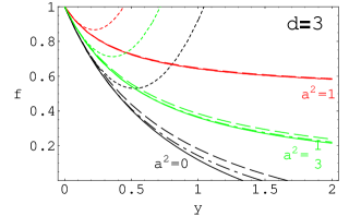
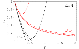
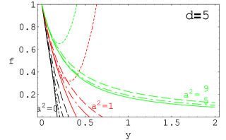
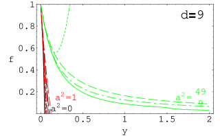
FIG. 1.: $f(y)$ is plotted against $y$ for $d=3$, $d=4$, $d=5$ and $d=9$. The solid line is obtained by the mean-field approximation, the broken line by the lowest-order Padé approximation, the dot-broken line by the next-to-leading Padé approximation, and the dotted line is the series expansion up to the second order.

REFERENCES

• [1] H. J. de Vega and N.  Sánchez, Phys. Lett. B490, 180 (2000), hep-th/9903236.
• [2] K. Shiraishi and T. Maki, Phys. Rev. D53, 3070 (1996).
• [3] A. Papapetrou, Proc. R. Irish Acad. A51, 191 (1947).
• [4] S. D. Majumdar, Phys. Rev. 72, 930 (1947).
• [5] R. C. Myers, Phys. Rev. D35, 455 (1987).
• [6] K. Shiraishi, J. Math. Phys. 34, 1480 (1993).
• [7] G. W. Gibbons and P. J. Ruback, Phys. Rev. Lett. 57, 1492 (1986).
• [8] R. C. Ferrell and D. M. Eardley, Phys. Rev. Lett. 59, 1617 (1987).
• [9] J. Traschen and R. Ferrell, Phys. Rev. D45, 2628 (1992).
• [10] K. Shiraishi, Nucl. Phys. B402, 399 (1993).
• [11] K. Shiraishi, Int. J. Mod. Phys. D2, 59 (1993).
• [12] Y. Degura and K.  Shiraishi, Effective field theory of slowly moving ‘extreme black holes’, Class. Quantum Grav. 17, 4031 (2000), hep-th/0006015.
• [13] G. W. Gibbons and R. E. Kallosh, Phys. Rev. D51, 2839 (1995).
• [14] R. Brooks, R. E. Kallosh, and T. Ortín, Phys. Rev. D52, 5797 (1995).
• [15] G. W. Gibbons, G. Papadopoulos, and K. S. Stelle, Nucl. Phys. B508, 623 (1997).
• [16] D. M. Kaplan and J. Michelson, Phys. Lett. B410, 125 (1997).
• [17] J. Michelson, Phys. Rev. D57, 1092 (1998).
• [18] J. Maldacena, J. Michelson, and A. Strominger, JHEP 9902 011 (1999).
• [19] J. Michelson and A. Strominger, JHEP 9909 005 (1999).
• [20] A. Maloney, M. Spradlin, and A. Strominger, Superconformal Multi-Black Hole Moduli Spaces in Four Dimensions, hep-th/9911001.
• [21] J. Gutowski and G. Papadopoulos, Phys. Lett. B472, 45 (2000).
• [22] J. Gutowski and G. Papadopoulos, Phys. Rev. D62, 064023 (2000).
• [23] R. Britto-Pacumio, J. Michelson, A. Strominger, and A. Volovich, Lectures on Superconformal Quantum Mechanics and Multi-Black Hole Moduli Spaces, hep-th/9911066, and references therein.
• [24] G. W. Gibbons, D. Kastor, L. A. J. London, P. K. Townsend and J. Traschen, Nucl. Phys. B416, 850 (1994).
• [25] G. W. Gibbons and K. Maeda, Nucl. Phys. B298, 337 (1982).
• [26] D. Garfinkle, G. Horowitz, and A. Strominger, Phys. Rev. D43, 3140 (1991); D45, 3888 (E) (1992).
• [27] N. Manton, Nucl. Phys. B400, 624 (1993).
• [28] P. A. Shah and N. Manton, Thermodynamics of Vortices in the Plane, J. Math. Phys. 35, 1171 (1994), hep-th/9307165.
• [29] F. K. Liu, MNRAS 281, 1197 (1996), astro-ph/9512061.
• [30] M. V. Medvedev and G. Rybicki, astro-ph/0010621.
• [31] P. Natarajan and D. Lynden-Bell, astro-ph/9604084.
Refer to captionRefer to caption Refer to captionRefer to caption