Non-linear harmonic generation in finite amplitude black hole oscillations

Abstract

The non-linear generation of harmonics in gravitational perturbations of black holes is explored using numerical relativity based on an in-going light-cone framework. Localised, finite, perturbations of an isolated black hole are parametrised by amplitude and angular harmonic form. The response of the black hole spacetime is monitored and its harmonic content analysed to identify the strength of the non-linear generation of harmonics as a function of the initial data amplitude. It is found that overwhelmingly the black hole responds at the harmonic mode perturbed, even for spacetimes with 10% of the black hole mass radiated. The relative efficiencies of down and up-scattering in harmonic space are computed for a range of couplings. Down-scattering, leading to smoothing out of angular structure is found to be equally or more efficient than the up-scatterings that would lead to increased rippling. The details of this non-linear balance may form the quantitative mechanism by which black holes avoid fission even for arbitrary strong distortions.

I Introduction

The dynamical behaviour of black holes near equilibrium has been clarified using classic, technically elaborate, perturbation theory (see e.g., [1]). In recent years there has been an interest in studying more general aspects of the dynamics of black holes as they would manifest e.g., in the merger of two black holes [2], or in other large deformation induced by an external agent. In this regime there are no readily available analytic tools and modern approaches advocate the use of discretization procedures. The most explored computational framework for the study of black hole dynamics dynamics [3] is facing a number of obstacles which limit the duration and accuracy of black hole simulations. Irrespective of difficulties, persistent work within this approach in the past decade [4, 5, 6] has uncovered important aspects of finite amplitude dynamics of black holes. A central suggestion of this effort has been that, in a larger than expected part of the parameter space, the physics of finite perturbations of black holes can be expressed in the language of infinitesimal perturbation analysis. It will be useful for what follows to review the main elements of this language: Linearised black hole perturbations are mapped into a problem of scattering off a positive potential which results from a combination of the angular momentum barrier with the one-way absorbing membrane of the horizon. Important role in the perturbative drama play the exponentially damped oscillating modes called quasi-normal modes (QNM). Those solutions form the mechanism by which weak perturbations of a black hole are radiated away, leading to a stationary remnant [7].

The discovery in [4, 5, 6] that finite perturbations of black holes, seen in either black hole-black hole or black-hole-gravitational wave systems, seem to emit their energy primarily through a linear channel was subsequently illuminated further with the interpretation of the numerically generated black hole spacetimes from the point of view of perturbation theory [7, 8]. There have been a number of more general studies [9, 10] investigating the validity of the basic picture for rotating and three-dimensional perturbations of black holes. This pioneering numerical work helped sharpen a number of questions surrounding non-linear black hole dynamics. Is there a genuinely non-linear regime? Is it visible to remote observers? What are the salient features of the evolution of an arbitrarily distorted black hole? Most intriguingly, how exactly does the non-linear evolution of a highly distorted black hole manage to avoid the perils of a fission and hence conform with the area theorem expectation [11]?

The present work aims to tackle those questions by approaching the computational challenge from a different angle, namely by using a geometric approach based on the characteristic initial value problem (civp). The civp was introduced in seminal work by Bondi and Sachs [12, 13] as an asymptotic, but non-perturbative, analysis of radiating spacetimes. Several variations have been proposed (see e.g., [14, 15, 16]) to enable global computations of general spacetimes. Those formulations typically share an excellent economy and adaptability to computations of quasi-spherical radiative spacetimes. Versions of the civp have been extensively used for the study of black hole dynamics in spherical symmetry, in connection with matter fields in particular (see. e.g.,  [17, 18, 19]). Higher dimensional studies based on the civp have been rapidly maturing over the past decade. An easily accessible review is given in [20].

The work presented here is based on the formal framework described in  [14]. The first adaptation of this formulation to the study of black holes using ingoing light-cone foliations was presented in [21], in a spherically symmetric setting. Subsequent developments led to long term stable three-dimensional computations of black holes [26]. In this paper, an algorithm developed originally for the study of regular axisymmetric spacetimes [23] has been adapted and applied to the study of finite amplitude black hole perturbations. The approach is described in Sec. II. The details of the numerical algorithm are substantially the same as in [23] and will not be repeated. The emphasis of the discussion will be instead on the new elements which adapt the method to the problem at hand. This includes, firstly, initial and boundary conditions and, secondly, a method for extracting the relevant physical information. Given the substantially different nature of solutions explored here compared to the tests in [23], re-calibrations and accuracy tests have been performed and pointed out where needed. In Sec. III the results of a parameter space survey covering initial data amplitude and a portion of the harmonic space are presented. The discussion begins with the study of selected waveforms and leads to the main topic, which is the quantification of energy transfered by various non-linear couplings. The relevance of the findings to the questions that motivated this work is assessed in the conclusions IV.

The usual unit conventions $(G=c=1)$ apply. The spacetime signature has been modified from timelike [23] to spacelike.

II Geometric and computational setup

1 Framework

The algorithm is based upon the civp for the Einstein equations in vacuum, using light cones emanating from a timelike worldtube. With the conventions of the Bondi-Sachs gauge, the explicit form of the metric element is

$$ds^{2}=-((1-{2M\over r})e^{2\beta}-U^{2}r^{2}e^{2\gamma})dv^{2}-2e^{2\beta}dvdr+\ 2Ur^{2}e^{2\gamma}dvd\theta+r^{2}(e^{2\gamma}d\theta^{2}+e^{-2\gamma}\sin^{2}\theta d\phi^{2}).$$ (1)

This form implies an axisymmetric spacetime with zero rotation. The metric variables $(\gamma,M,\beta,U)$ are functions of the coordinates $(v,r,\theta)$ only. The formulation of a boundary initial value problem follows the lines of [14], with light-cones emanating from a timelike worldtube at a finite radius and proceeding inwards, to intercept the black hole horizon (see Fig. 1). This setup may be considered as a straightforward generalisation of the well known family of ingoing Eddington-Finkelstein coordinate system to axisymmetric distorted black holes.

The vacuum Einstein equations decompose into three hypersurface equations and one evolution equation (the conservation equations along the world-tube will not be used and are omitted here). The overall form of the equations is given in symbolic notation (the reader is referred to [22, 23] for the detailed expressions as they are used in the code):

$$\Box\,^{(2)}\psi = {\cal H_{\gamma}}(M,\beta,U,\gamma),$$ (2)

$$\beta_{,r} = {\cal H}_{\beta}(\gamma),$$ (3)

$$U_{,rr} = {\cal H}_{U}(\beta,\gamma),$$ (4)

$$M_{,r} = {\cal H}_{M}(U,\beta,\gamma),$$ (5)

where $\Box\,^{(2)}$ is an appropriate 2-dimensional wave operator acting on the $(v,r)$ sub-manifold, $\psi=r\gamma$, and the symbols $H_{X}$ denote reasonably lengthy right-hand-side contributions. Free initial data for $\gamma$ on an ingoing light-cone $\cal{N}$ lead, with the integration of the radial hypersurface equations (3,4,5), to the complete metric along $\cal{N}$. This then enables the computation of $\gamma$ on the next light cone, with the use of the evolution equation (2). This system of equations is extremely economical, given that it encodes the full content of the Einstein equations for the assumed symmetry.

2 Linearised limit

Before proceeding to the details of setting up the initial value problem, there is some merit in discussing the linearised limit of the equations (2,3,4,5) around a spherical black hole background of mass $M_{0}$. The linearised limit around Minkowski spacetime ($M_{0}$) was analysed in [12, 23] and various reductions of the dynamics to the wave equation have obtained. For non-zero background mass, one obtains the coupled system

$$2\psi_{,rv}+((1-\frac{2M_{0}}{r})\psi_{,r})_{,r} = -\frac{2M_{0}}{r^{2}}\gamma-\frac{1}{2r}(r^{2}\sin\theta(\frac{U}{\sin\theta})_{,\theta})_{,r}\,,$$ (6)

$$(r^{4}U_{,r})_{,r} = -2\frac{r^{2}}{\sin^{2}\theta}(\sin^{2}\theta\gamma)_{,r\theta}\,.$$ (7)

Physically, from the assumptions leading to the metric element, those equations describe axisymmetric, even parity perturbations of Schwartzschild black holes [1]. They also ought to be reducible to a single equation in the spirit of perturbation theory. The presence of a black hole affects the evolution of the shear of the ingoing light-cone primarily with the modification of the slope of outgoing characteristics, which vanishes at the horizon. There is a potential term, specific to the spin-2 gravitational perturbations. The remaining RHS term in the $\gamma$ equation, together with the $U$ equation, form effectively the angular momentum barrier.

With the minimal structure of the equations now transparent, in the restoration of non linear terms, one can identify at least three distinct alterations: Firstly, a modification of the light-cone structure, affecting the principal part of the equation and hence the propagation speed of signals. Secondly, a modulation of the existing spherical potential term. For example, the mass aspect function $M$ acquires angular structure. Thirdly, quadratic couplings emerge and act as source terms, e.g., in the evolution equation. The combined effect of the last two agents will be the mixing of oscillation modes of different geometrical characteristics.

3 Boundary and Initial Data

Within an ingoing light-cone framework, there are two possible prescriptions for setting up initial and boundary data for the study of the response of a black hole to perturbations. In the first, akin to a scattering study, the initial advanced time light cone $\cal{N}$ has trivial background data. Incoming gravitational radiation is introduced at the world tube $\cal{W}$ through the specification of the unconstrained $\gamma(v,\theta)|_{\cal{W}}$ function. A self-consistent evolution of the boundary data is then achieved by the time-integration of the conservation conditions along the world-tube. In the second approach, which may be called a perturbation study, the free data are specified on $\cal{N}$, whereas $\cal{W}$ is kept with trivial data. The two approaches are closely linked, since the scattering of incoming radiation will immediately lead to outgoing perturbations. Still, the perturbation approach is computationally simpler, since it avoids the integration of the conservation conditions. This is the approach used here.

The world-tube boundary conditions are simple but central to the setup of the physical problem. A non-rotating unit-mass black hole is prescribed at $\cal{W}$ by setting $M(v,r_{\cal{W}})=1$ and all other fields equal to zero. Such a condition is not in general compatible with a spacetime in which outgoing radiation is filtering through the worldtube. Minimally, such radiation would be diminishing the mass contained inside the worldtube, and $M(v,r_{\cal{W}})$ would not be constant. Hence, for consistency, evolutions must be restricted in time so that the neighbourhood of the world-tube is unperturbed by local flux of radiation. Fulfilling this condition is entirely possible and will always be the case in the results presented here.

The free initial data on the ingoing light cone $\cal{N}$ are captured by a single real function of two variables $\gamma(r,\theta)$. For a spherical unperturbed spacetime this function is identically zero. The radial profile of a perturbation must be chosen so that the evolution conforms with the constraint discussed in the previous paragraph. This leads to the adoption of an exponentially decaying profile, as a model of a localised disturbance superposed on a black hole. Clearly, for perturbations arising in astrophysical systems, the prior history of the system is likely to have produced a more extended perturbation, arguably though, of very small amplitude. A Gaussian profile, centred at a radius $r_{c}$ is hence chosen as a generic representative, and this freedom will not be explored here any further. Comparison between different values for $r_{c}$ suggests that values close to $r=3M$ are more effective in generating outgoing non-linear response and this value will be adopted throughout.

The angular profile of the initial data will play a key role in the following discussion. The only constraint is that the function a has suitable falloff at the pole $y=\pm 1$, consistent with the fact that $\gamma$ is a spin-2 scalar representing the everywhere regular intrinsic metric of topological spheres of constant r. This fall-off condition is equivalent to requiring that the angular decomposition of $\gamma$ in harmonics starts with at least a quadrupole term. The spin harmonics relevant to this decomposition are discussed in detail in [24]. In axisymmetry, a convenient expression for the basis functions is given by

$$Y_{2l0}=\left(\frac{(l-2)!(2l+1)}{4\pi(l+2)!}\right)^{1/2}(P_{l,\theta\theta}-\cot\theta P_{l,\theta})$$ (8)

where $Y_{2lm}$ denotes an $(l,m)$ harmonic of spin $2$ and $P_{l}$ are the Legendre polynomials.

The free specification of initial data, one of the virtues of the civp, permits the introduction of pure angular harmonic dependence, by means of expressions like, e.g.,

$$\gamma(r,\theta)=\frac{\lambda}{\sqrt{2\pi}\sigma}e^{-(r-r_{c})^{2}/\sigma^{2}}Y_{2l0}(\theta)\,.$$ (9)

The multipole index $l$ of the initial data will be referred to as the primary harmonic, as it is to be expected that it will play an important role in the response of the black hole geometry to the perturbations. The physical content of such data is essentially a local distortion of the ingoing light-cone, with prescribed angular structure and amplitude. The claim that the spacetime constructed by this approach is actually a distorted black hole is made geometrically more precise by the introduction of the concept of a marginally trapped 2-surface (MTS) on a given ingoing light-cone $\cal{N}$. An MTS is defined, in this context, as the two-parameter radial function $R(r,\theta)$ on which the expansion $\Theta=2\nabla^{\alpha}l_{\alpha}$ of an outgoing null ray pencil $l^{\alpha}$ vanishes [21]. Using a relaxation method for the solution of equation $\Theta=0$ one obtains indeed a distorted initial MTS, showing curvature dependent on the amplitude of the data. The invariant analysis of the intrinsic geometry and dynamics of the MTS are interesting problems in themselves and deserve separate study.

4 Extraction of the non-linear response

The evolution of the initial data leads, in general, to radiation emission towards both infinity and the horizon. Here the focus will be on the outgoing, in principle observable, part. The non-linear response of the black hole to the initial perturbation will be encoded quite legibly in the angular harmonic decomposition of the outgoing solution. A strategy to isolate this information is outlined here.

The metric perturbation encoded in $\gamma$ can be decomposed in spin-2 harmonics as

$$\gamma(v,r,\theta)=\sum^{\infty}_{l=2}\gamma_{l}(v,r)Y_{2l0}(\theta)\,,$$ (10)

which is inverted as

$$\gamma_{l}(v,r)=2\pi\int^{1}_{-1}\gamma(v,r,y)Y_{2l0}(y)dy\,,$$ (11)

using the orthonormality of the spin-2 harmonics and introducing $y=-\cos\theta$. At this stage the decomposition is non-perturbative, i.e., it does not depend on $\gamma$ being small and can be can be carried out across the entire light-cone. The set of functions $\gamma_{l}(v,r)$ is effectively capturing all the information about the given spacetime. For non-linear evolutions, this set includes more than one harmonics, even if the initial data are set to a single (the primary) harmonic dependence. The new harmonics will be referred to as the secondary harmonics. In numerical practice, this decomposition is obtained via an eighth-order accurate (in $\Delta y$) angular integration of the grid data.

A good indicator of non-linear processes near the black hole is the amount of energy emitted in secondary harmonics. In the present setup the foliation does not extend to infinity, hence the extraction of an energy estimate for an outgoing solution must resort to an approximate expression. The task is straightforward, due to the adapted form of the metric element (i.e., spherical coordinates, light-cone gauge). Further, sufficiently far from the black hole (but inside the world-tube), the outgoing radiation is weak in amplitude and the spacetime is close to a Schwartzschild spacetime in its standard ingoing Eddington-Finkelstein form. At that radius, denoted as the observer radius $r_{o}$, and forming a timelike worldtube of area $4\pi r_{o}^{2}$, the news can be approximated by $c(v)=\psi(v)=r_{o}\gamma(v)$. From this, it follows that the total (negative) energy flux crossing the observer will be approximating Bondi’s energy flux integral

$$\frac{dE_{tot}}{dv}=-\frac{1}{4\pi}\oint(\psi_{,v})^{2}\sin\theta d\theta d\phi\,.$$ (12)

An expression for the total energy emitted in each angular mode $l$ after an evolution to a final time $T$ is given by

$$E_{l}(T)=\frac{1}{4\pi}r^{2}_{o}\int^{T}_{0}(\gamma_{l,v})^{2}dv\,.$$ (13)

Given the availability of the complete spacetime, the device developed here is but a partial probe whose usefulness rests on its quantitative nature.

Other non-linear effects will include, for example, deviations of the oscillation frequencies from the weak field limit. Those effects need careful differentiation from the natural inclusion of higher overtones, which are present in the initial response of linearised perturbations as well. They also appear, at first sight, difficult to quantify and for this reason will play a lesser role in this study.

5 Computational aspects

The computational algorithm follows closely that developed in [23] and differs effectively only in the boundary treatment and in the sense in which the integration proceeds (here towards smaller radii). The algorithm was shown second order accurate in the non-linear regime using a static boost-symmetric solution (SIMPLE) and in the linear regime using exact decaying multipole solutions for harmonics up to $l=6$. In addition the consistency of the evolution was checked using global energy conservation. The black hole dynamics problem is sufficiently different and computationally challenging [25] though, that a re-calibration of the code has been performed. It was found that, for the high resolution grid used below, the primary harmonic can safely be captured to better than 1%. The good overall accuracy of the code does not automatically guarantee the correct capturing of the non-linear effects, as those are emergent. For this reason, quantitative statements about such effects will be individually certified as will be shown below.

The solution procedure involves about 350 lines of essential code. The numerical grid is equidistant in both the radial $r$ and the angular $y=-\cos\theta$ coordinates. Accurate calculations involve 2000 radial grid points covering the radial domain from $r_{\mbox{min}}=1.8M$ to $r_{\mbox{max}}=60M$ and 90 grid points covering the angular domain $y=[-1,1]$. This corresponds to a $\Delta r=0.03M$ and $\Delta\theta=0.02$ at the equator. Evolution for a total time of $120M$ consumes about 30min of a 666Mhz Alpha CPU, at roughly 240 Mflops. About 45% of that time is spend on the update of the dynamical variable $\gamma$, with the rest being distributed among the hypersurface integrations and auxiliary tasks. For the assessment of the accuracy of the results, evolutions using a second grid, with half the resolution (i.e.,$(1000\times 45)$) in both directions, will be used throughout.

The numerical evolution is formulated in an explicit manner, and is hence subject to a CFL stability condition. In the black hole case under consideration the origin of the coordinate system is not the vertex of a light-cone, and the constraint imposed by the CFL condition is weaker. As usually the case in explicit methods, it becomes linear in the grid spacing instead of quadratic condition found in [23]. The computational cost and accuracy of the simulations, is comparable to axisymmetric (2+1) calculations based on linearised theory [27].

III Non-linear evolution results

It is appropriate to start with the venerable quadrupole perturbation ($l=2$ in equation (9)), and fix $\sigma=0.5$, $r_{c}=3.0$. This introduces a finite perturbation sitting squarely on the potential barrier of classic perturbation theory. The various runs (the complete list is given in Table I), are parametrised by the amplitude of the initial data, $\lambda$. The range of amplitudes explored is defined on the one end by the requirement that non-linear effects are stronger than numerical truncation error and on the other by the necessity that the evolution maintains a smooth, well behaved, ingoing light-cone foliation. For sufficiently strong data the geometry is seen to develop kinks, along specific angles, starting first at the innermost radial points (one can always hasten the death of the foliation by evolving deeper inside the horizon). For evolutions just below the breakdown amplitude, those features require increasingly larger angular resolution to resolve. The strong field effects responsible for the caustic formation at the inner edges of the domain have not been found to be reflected on the actual observed non-linear behaviour. For this reason the results presented here do not attempt to capture the precise limits of the caustic-free regime.

Illustrated here is the strongest case, $\lambda=0.25$. The response of the black hole to this perturbation is shown in Fig. 2, as registered by an observer located at $20M$. The arrival time of the primary response is roughly twice the radial separation of the observer from the black hole (40M), reflecting the fact that outgoing light waves propagate at coordinate speed 1/2 in an ingoing light-cone framework. The primary (quadrupole) response carries, for this amplitude, almost 10% of the black hole mass in radiation. An $l=2$ perturbation carries no linear momentum (it is reflection symmetric with respect to the equator) and hence one does not expect to see an output of odd harmonics. Given the large amount of radiated energy, one would expect that the couplings in the RHS of the evolution equation (2) will generate some even-harmonic signal. In this case, given that the primary is the lowest allowed harmonic, all secondary response will have higher $l$ values (up-scattering in $l$ space) and will therefore tend to create further ripples in the predominantly spherical black hole geometry. A first taste of quantitative result follows from the observed amplitudes of the secondary harmonics ($l=4,6$): They are respectively one and two orders of magnitude lower in amplitude. Odd harmonics do not appear, up to roundoff error.

The typical damped oscillatory behaviour known from linearised analysis is visible here also for large finite perturbations. Looking closer into the secondaries one notes that, with respect to the primary wave, the global maxima of the secondary harmonics i) are slightly delayed and ii) have phase reversals (i.e., the global maxima alternate in sign). Given that the primary wave has a peak at negative amplitude, the origin of the $l=4$ secondary waves in quadratic coupling may explain the phase reversal. Similarly, the cubic coupling for the $l=6$ wave may account for the second reversal seen there. This claim will be strengthened by the analysis of the functional dependence on the initial data amplitude later on. The evident time delay is harder to be accounted for.

Proceed next to a family of runs where the initial data are set to an $l=3$ harmonic. This case differs markedly in physical content from the one described previously, as the initial data do not exhibit equatorial reflection symmetry and posses net linear momentum. In addition, the fact that the $l=3$ harmonic is not the lowest allowed oscillation mode raises the possibility that the secondary harmonics have both higher and lower angular structure. The down-scattering to lower $l$ values is particularly interesting, as it represents a mechanism by which energy is lost from the primary harmonic to a smoother configuration. The response, for a family of data of identical radial profile is monitored again, at the same finite radius. The five different profiles shown in Fig. 3 are the time-dependent amplitudes of the harmonically decomposed signal at the observer (harmonics $l=2$ to 6) for an amplitude of $\lambda=0.25$. The strongest signal corresponds to the multipole geometry of the initial perturbation. The present situation is in contrast with the previous example, where the equatorial reflection symmetry (zero linear momentum) of the primary mode was reflected in all secondaries. Despite the fact that the primary mode carries linear momentum, the secondaries are anything but reflection anti-symmetric. In fact, the nearest antisymmetric mode ($l=5$) is the weakest in amplitude. Whereas the overall damped oscillation theme is still dominant, some subtleties are more apparent here. This can be seen most easily in the large change in the periods of the $l=2$ mode between the former and latter parts of the signal and also in the significant modulation seen in the $l=5$.

It is not entirely clear how to effectively characterise damped oscillating signals with brief duration and strong variability. The sixth panel in Fig. 3 attempts an, at least, qualitative analysis in the following manner. For each harmonic, the zero crossing of the signal at the observer is recorded. Successive zero crossings provide an instantaneous value for the half-period of the oscillation. This is plotted as a function of time, illustrating in this manner the evolution of the signal frequency in time. The horizontal lines in that panel are half-periods for QNM oscillations of even parity perturbations of Schwartzschild black holes [1]. The QNM periods are $T=16.81,10.48,7.76,6.21,5.18$ (in units of M) for perturbations of $l=2,\cdots,6$ type, respectively. The very strong (doubling) of the frequency of the $l=2$ harmonic is notable. The frequency asymptotes to the weak field value, but only after substantial evolution time. The primary harmonic ($l=3$) is less strongly evolving and attains its weak field value earlier on. The $l=5$ response also exhibits the strong time evolution seen in the quadrupole and reaches its weak field value late in the evolution. The $l=4$ periods are problematic and only the few initial estimates are shown. This is despite the, at first sight, normal appearance of the signal. The reason has been traced to the secular evolution of the black hole remnant (region IIb of Fig. 1) which affects the time derivative of the field at the observer. Recall that the effective energy content between the world-tube and the horizon acts tidally on the black hole and distorts it. There is a small physical amount of energy loss, as radiation is absorbed by the horizon, and possibly to numerical dissipation. Both effects would lead to a slow evolution of the remnant, which is captured by the time dependent value of $\gamma_{,v}$ at the observer. The effect will be more pronounced for harmonics that match closer to the geometry of the remnant (here the $l=4$) and are weak in amplitude. The tail of the $l=4$ signal is seen not to asymptote to zero, but rather to a small negative value. Examining the second time derivative and/or using further placed observers may help reduce this effect, but frequency considerations are not central to this study and this is not pursued further. An oscillatory effect of possibly the same or similar origin affects the late time periods of the ($l=6$) harmonic which are seen to oscillate about the QNM value.

Keeping with the same overall setup, the evolution of an $l=4$ primary is studied. This case is physically close to the quadrupole one, except that here it is possible to have down-scattering to the quadrupole harmonic. This adds new scope to the analysis, as it allows comparison of the up-scattering mechanism from 2 to 4, to the down-scattering from 4 to 2. One relevant difference of the $l=4$ primary is that caustics appear to be forming here for weaker data (about a tenth the total energy of the $l=2,3$ cases). This is possibly due to more efficient focusing of ingoing rays by data of same total energy if those data have angular structure.

The cumulative energy calculations for the three scenarios are presented in Table I. This table is the central result of this paper and hence warrants some discussion. The range of chosen amplitudes has already been justified. The range of harmonics studied is a compromise between reasonable completeness and finite resources. The error bars are important in establishing confidence in those particular numbers. They are evaluated by performing the same calculation again, with exactly twice the resolution and taking the difference in calculated energy as a measure of confidence. Numerical effects can artificially generate or suppress harmonics, e.g., through boundary effects and dispersion. In addition, dissipation will affect the amplitudes. Low resolution is particularly dangerous for down-scattered modes, and it is found that there is a minimum angular resolution required for the non-linear signal to rise above the truncation error. The error bars serve as a guard against attempting to resolve too subtle an effect.

For the range of data studied, the energy in any mode is always a monotonically increasing function of the initial data amplitude. There is energy in all modes, except for those couplings excluded by the conservation of linear momentum. The forbidden couplings typically show energy well below $10^{-20}$, which suggests an origin in roundoff error. Indirectly this suggests that the discretized version of the equations (and its implementation) respects a conservation law as well. Almost the entire content of Table I can be grasped easily by putting the data on a log-log graph as in Fig. 4. This graph excludes the primary harmonic data (diagonal elements of the table), as those encode how much energy is subtracted from the mode as a function of initial data amplitude, whereas the off-diagonal terms capture how much energy is added to the mode. It is immediately seen that the energy versus amplitude relation is a power law for all cases, but with different slopes and normalisations that can be described by

$$E_{ll^{\prime}}=\epsilon_{ll^{\prime}}\lambda^{s_{ll^{\prime}}}M\,,$$ (14)

where the first (second) indices denote the primary (secondary) harmonics respectively. The exponent $s_{ll^{\prime}}$ will, in general, follow from the type of coupling, i.e., it reflects a geometric feature of the theory. The normalisation factor $\epsilon_{ll^{\prime}}$ captures the efficiency of the coupling and will be much closer associated with the detailed structure of the solution, in the region where the coupling is active. With linear best fits to the data points, one can estimate values for $(s_{ll^{\prime}},\epsilon_{ll^{\prime}})$ (Table II).

Upon examining the table of numerical fits it is clear that the quadratic couplings dominate the various transitions (a quadratic coupling generates a fourth order energy scaling). There are two examples of higher couplings (cubic in the amplitude), namely the $2\rightarrow 6$ and the $3\rightarrow 5$. There are several important points about efficiencies: The most efficient process is a down-scattering, namely the $4\rightarrow 2$ coupling. This means, in particular, that for an equal amplitude input, there is more non-linear energy loss from an octupole to a quadrupole than the reverse, by a factor of more than two. There is near parity between the $3\rightarrow 2$ and $3\rightarrow 6$ couplings, i.e., this shows that the non-linear energy drain from the momentum-carrying $l=3$ mode is almost equally split between the zero-momentum $l=2$ and $6$ modes.

IV Summary and Discussion

A computational framework for the study of finite amplitude black hole perturbations has been developed on the basis of the characteristic initial value problem for the Einstein equations in an ingoing light-cone setup. A stable code with controllable resolution requirements was configured for delivering better than 1% signal accuracy for angular structures up to $l=6$. Finite amplitude perturbations were studied for total radiative energies up to 10% of the black hole mass. The examination of the distribution of energy in non-linearly generated radiative modes provides some new insights on the dynamics of strongly perturbed black holes.

The main conclusions are that: i)The energy transfered through various couplings is found to obey simple power law scalings, up to the amplitudes studied. ii) The non-linear couplings are inefficient in channelling energy away from the primary mode. iii) Up-scattering in $l$ space (tendency to form ripples in the geometry) and down-scattering (tendency to smooth the geometry) are found to have comparable efficiencies, with the distinct possibility that non-linear smoothing is actually dominant. iv) Various non-linear effects are present during roughly the first 30M of evolution, including relative time delays of the different harmonics, phase reversals, and strong frequency evolution of oscillations before they reach their asymptotic QNM value. The early periods are always smaller than the final QNM value, compatible with a picture in which the initial black hole is smaller.

A relevant question is whether one can reasonably extrapolate to an arbitrary amplitude regime. The studies of black hole head-on collisions are probing a different, possibly stronger, regime of distortions (a proper assessment would require a study of invariants of the horizon geometry). It seems that the phenomenology of the response in such simulations is compatible with the picture laid out here. I.e., collisions are genuinely non-linear evolutions, which fail to generate visibly non-linear signals because of inefficient off-diagonal couplings. The fairly independent evolution of individual harmonic modes, a true non-linear property of the Einstein equations as applied to the black hole system, clarifies the larger than expected domain of applicability of infinitesimal black hole perturbations to collisions.

One can sharpen the picture by discussing a hypothetical non-linear black hole regime that, apparently, does not happen. Motivated by other non-linear hyperbolic systems, one could be excused to imagine an efficient and unhindered energy cascade towards large $l$. The geometry of a sufficiently strong initial quadrupole perturbation could say “pinch” along certain angles, in a region visible to the exterior, hence emitting large amounts of energy in higher frequencies. This does not happen. Up-scattering efficiencies, besides failing to dent the energy carried by the primary mode, seem to be also kept in check by the sligthly more efficient down-scattering processes. The conjecture is that this “diagonally dominant” non-linear transfer matrix, with its appropriately tuned weights above and below the diagonal, is ultimately responsible for enforcing the non-linear stability of a black hole to arbitrary distortions.

Input Data		Output Energy in Harmonics (in units of M)
$l$	$\lambda$	$E_{2}$	$E_{3}$	$E_{4}$	$E_{5}$	$E_{6}$
	0.25	$(0.97\pm 0.01)10^{-1}$	0	$(0.41\pm 0.01)10^{-2}$	0	$(0.42\pm 0.04)10^{-3}$
	0.177	$(0.45\pm 0.01)10^{-1}$	0	$(0.98\pm 0.01)10^{-3}$	0	$(0.47\pm 0.02)10^{-4}$
2	0.125	$(0.21\pm 0.01)10^{-1}$	0	$(0.23\pm 0.01)10^{-3}$	0	$(0.52\pm 0.01)10^{-5}$
	0.0884	$(0.10\pm 0.01)10^{-1}$	0	$(0.54\pm 0.01)10^{-4}$	0	$(0.60\pm 0.01)10^{-6}$
	0.0625	$(0.51\pm 0.01)10^{-2}$	0	$(0.13\pm 0.01)10^{-4}$	0	$(0.71\pm 0.01)10^{-7}$
	0.25	$(0.87\pm 0.05)10^{-4}$	$(0.11\pm 0.01)10^{-1}$	$(0.23\pm 0.01)10^{-4}$	$(0.36\pm 0.01)10^{-6}$	$(0.87\pm 0.02)10^{-4}$
	0.177	$(0.19\pm 0.01)10^{-4}$	$(0.54\pm 0.01)10^{-2}$	$(0.57\pm 0.03)10^{-5}$	$(0.45\pm 0.01)10^{-7}$	$(0.22\pm 0.01)10^{-4}$
3	0.125	$(0.47\pm 0.03)10^{-5}$	$(0.27\pm 0.01)10^{-2}$	$(0.14\pm 0.01)10^{-5}$	$(0.55\pm 0.01)10^{-8}$	$(0.53\pm 0.01)10^{-5}$
	0.0884	$(0.12\pm 0.01)10^{-5}$	$(0.14\pm 0.01)10^{-2}$	$(0.35\pm 0.02)10^{-6}$	$(0.70\pm 0.01)10^{-9}$	$(0.13\pm 0.01)10^{-5}$
	0.0625	$(0.29\pm 0.02)10^{-6}$	$(0.67\pm 0.01)10^{-3}$	$(0.89\pm 0.05)10^{-7}$	$(0.86\pm 0.03)10^{-10}$	$(0.33\pm 0.01)10^{-6}$
	0.075	$(0.75\pm 0.04)10^{-4}$	0	$(0.86\pm 0.01)10^{-2}$	0	$(0.14\pm 0.02)10^{-4}$
	0.053	$(0.18\pm 0.02)10^{-4}$	0	$(0.42\pm 0.01)10^{-2}$	0	$(0.33\pm 0.04)10^{-5}$
4	0.0375	$(0.43\pm 0.04)10^{-5}$	0	$(0.20\pm 0.01)10^{-2}$	0	$(0.79\pm 0.10)10^{-6}$
	0.0265	$(0.10\pm 0.01)10^{-5}$	0	$(0.10\pm 0.01)10^{-2}$	0	$(0.19\pm 0.02)10^{-6}$
	0.0187	$(0.25\pm 0.03)10^{-6}$	0	$(0.50\pm 0.01)10^{-3}$	0	$(0.46\pm 0.06)10^{-7}$

TABLE I.: Cumulative data for energy transfer between harmonic modes in non-linear black hole perturbations. The left column shows the type of initial distortion (harmonic index and amplitude). The highest amplitude in each $l$ family corresponds roughly to the strongest data that will evolve without forming a caustic near the horizon. For $l=2$ and $l=3$ the energy carried by such data is about 10% of the black hole mass. For $l=4$ it is an order of magnitude less. The off-diagonal elements of the table tell the story of secondary harmonic generation, towards smoothing or rippling the primary. They have a variety of scalings and efficiencies, which will be captured better in the graph of Fig.4. The zero values in the entries denote roundoff generated measurements that are typically less than $10^{-20}$. Error estimates are based on results from lower resolution runs. Error values below 1% have been rounded up to that value.

Coupling $ll^{\prime}$	Exponent $s_{ll^{\prime}}$	Efficiency $\epsilon_{ll^{\prime}}$
24	4.16	1.32
26	6.27	2.47
32	4.02	$2.07\,10^{-2}$
34	4.00	$5.49\,10^{-3}$
35	6.01	$1.51\,10^{-3}$
36	4.02	$2.31\,10^{-2}$
42	4.11	$3.11$
46	4.11	$2.07$

TABLE II.: Derived coupling exponents and efficiencies based on the data of Table I. Eight couplings are studied in total, listed with a compact notation in the left column. Six couplings are seen to be quadratic, the other two being cubic (the energy scales as the square of the amplitude). The efficiencies range in value. The most efficient quadratic process (at unit amplitude this would be dominant quadratic process) transfers energy from the octupole harmonic to the quadrupole one. Near unit amplitudes, the cubic up-scatterings would appear to generally dominate. It is highly likely though that the examination of an $l=6$ primary evolution would reveal even more efficient cubic down-scatterings.

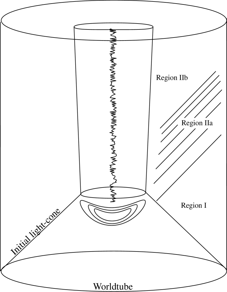
FIG. 1.: Spacetime diagram illustrating the main aspects of the geometric and computational setup of the problem. The foliation is based on advanced time, using ingoing light-cones which emanate from a world-tube. The geometry at the world-tube is kept fixed at all times and is given by the Schwartzschild values. The initial ingoing light cone is distorted with the specification of an arbitrary amount of shear. The sole constraint comes from the requirement that the ingoing cone will not develop a caustic before one reaches a marginally trapped surface. The evolution generates a dynamic spacetime, with the initial data scattering both towards and away from the black hole. For initial data that are restricted to zero outside some given radius, there is clean propagation into the unperturbed region I, where the spacetime is Schwartzschild. The outgoing gravitational disturbance (region IIa) can be intercepted by an “observer” at a suitable radius and analysed with respect to structure. At late times, of the order of hundreds of M, a slowly evolving “remnant” appears in the inner region IIb. The portion of the spacetime that emerges there represents a distorted black hole, the agent of distortion being the outward propagating gravitational radiation energy that intervenes between the horizon and the spherical worldtube.

FIG. 2.: Gravitational radiation signals from a black hole perturbed with quadrupole initial data. The three different panels show the time-dependent amplitudes of the harmonically decomposed signal at the observer (harmonics $l=2,4$ and 6). The upper panel shows the strongest response (primary harmonic). The tail of all modes exhibits the typical damped oscillatory behaviour known from linearised analysis. There are large amplitude differences between the various modes which are quantified in detail. The higher harmonics exhibit a time lag of the first peak with respect to the primary excitation. Note also the successive phase reversal in the secondary harmonics. The primary signal has a negative global maximum which becomes a positive one for $\psi_{4,v}$ and again a negative one for $\psi_{6,v}$. For the purpose of illustrating visually the code accuracy, each panel shows two lines, a solid one corresponding to the high-resolution grid and a dotted one corresponding to half that resolution.

FIG. 3.: Gravitational radiation signals from an $l=3$ distortion of a black hole. Five different panels show the time-dependent amplitudes of the harmonically decomposed signal (harmonics $l=2$ through 6). The panel at the upper-left corner shows the primary harmonic. One notes immediately that for a primary mode with intrinsic linear momentum (odd $l$ values), all secondary modes are excited. Again the amplitudes of the various harmonics vary considerably (note the multiplication factors denoted in the panels). The overall damped oscillation picture is still recognisable but strong modulations are visible even with cursory inspection. The sixth panel (lower-right corner) illustrates a time domain analysis of the frequency content of the signals in the following fashion: Illustrated are the zero crossings of the various harmonics as a function of arrival time. Filled circles, diamonds and squares correspond to $l=2,3,5$ respectively. Crosses denote $l=4$ and Pluses denote $l=6$. The horizontal lines denote predicted theoretical values for half-periods from linearised even parity perturbations. There is generally good agreement, after about 30M, but substantial deviations initially. The $l=4$ case exhibits some peculiarity which is discussed in the text.

FIG. 4.: Energy emitted in secondary harmonics as a fraction of the black hole mass, versus the amplitude of the initial data. The straight lines are linear best fits, slopes and intercepts are given in Table II. All data points fit well with power laws, reflecting polynomial underlying couplings. The amplitude range of the $l=4$ family terminates at lower value than the $l=2,3$ families because of higher sensitivity to caustic formation. One of the most remarkable facts uncovered in this non-linear coupling analysis is that apparently the down-scattering of $l=4$ to $l=2$ is the most efficient process among those studied.

REFERENCES

- [1] S. Chandrasekhar, The Mathematical Theory of Black Holes (Oxford University Press, Oxford, 1982).
- [2] A. Abrahams et al., The Binary Black Hole Grand Challenge Alliance, Phys.Rev.Lett. 80, 1812 (1998).
- [3] L. Smarr, in Sources of Gravitational Radiation, edited by L. Smarr (Cambridge University Press, Cambridge, England, 1979).
- [4] A. Abrahams, D. Bernstein, D. Hobill, E. Seidel, and L. Smarr, Phys. Rev. D 45, 3544 (1992).
- [5] P. Anninos, D. Hobill, E. Seidel, L. Smarr, and W-M. Suen Phys. Rev. Lett. 71, 2851 (1993).
- [6] D. Bernstein, D. Hobill, E. Seidel, and L. Smarr, Phys. Rev. D 50, 3760 (1994).
- [7] R. H. Price and J. Pullin, Phys. Rev. Lett. 72, 3297 (1994).
- [8] R. Gleiser, C. Nicasio, R. H. Price, and J. Pullin, Phys. Rev. Lett. 77, 4483 (1996).
- [9] S. Brandt and E. Seidel, Phys.Rev. D 52, 870 (1995).
- [10] K. Camarda and E. Seidel, Phys.Rev. D 59, 064019 (1999).
- [11] S. W. Hawking and G. F. R. Ellis, The large scalar structure of space-time, (Cambridge University Press, Cambridge, 1973).
- [12] M. van der Burg, H. Bondi, and A. Metzner, Proc. R. Soc. London Ser. A 269, 21 (1962).
- [13] R. K. Sachs, Proc. R. Soc. London Ser. A 270, 103 (1962).
- [14] L. A. Tamburino and J. H. Winicour, Phys. Rev. 150, 1039 (1966).
- [15] R. d’Inverno and J. Smallwood, Phys. Rev. D 22, 1223 (1980).
- [16] R. Bartnick, Class. Quant. Grav. 14, 2185 (1997).
- [17] C. Gundlach, R. Price, and J. Pullin, Phys. Rev. D 49, 890 (1994).
- [18] R. S. Hamade and J. M. Stewart, Class.Quant.Grav. 13, 497 (1996).
- [19] P. Papadopoulos and J. A. Font, Phys.Rev.D 63, 044016 (2001).
- [20] J. Winicour, Living Reviews
- [21] R. Gómez, P. L. Marsa, and J. Winicour, Phys. Rev. D 56, 6310 (1997).
- [22] R. Isaacson, J. Welling, and J. Winicour, J. Math. Phys. 24, 1824 (1983).
- [23] R. Gómez, P. Papadopoulos, and J. Winicour, J. Math. Phys. 35, 4184 (1994).
- [24] R. Penrose and W. Rindler, Spinors and Space-Time, Vols. 1 and 2 (Cambridge University Press, Cambridge, 1984).
- [25] P. Papadopoulos, E. Seidel, and L. Wild, Phys.Rev.D 58, 084002 (1998).
- [26] Gomez et al., Phys.Rev.Lett 80, 3915 (1998).
- [27] W. Krivan, P. Laguna, P. Papadopoulos, and N. Andersson, Phys.Rev.D 56, 3395 (1997).