Local and global properties of conformally flat initial data for black hole collisions

Abstract

We study physical properties of conformal initial value data for single and binary black hole configurations obtained using conformal-imaging and conformal-puncture methods. We investigate how the total mass $M_{tot}$ of a dataset with two black holes depends on the configuration of linear or angular momentum and separation of the holes. The asymptotic behavior of $M_{tot}$ with increasing separation allows us to make conclusions about an unphysical “junk” gravitation field introduced in the solutions by the conformal approaches. We also calculate the spatial distribution of scalar invariants of the Riemann tensor which determine the gravitational tidal forces. For single black hole configurations, these are compared to known analytical solutions. Spatial distribution of the invariants allows us to make certain conclusions about the local distribution of the additional field in the numerical datasets.

04.25.Dm, 04.70.-s

I Introduction

The problem of initial conditions (initial Cauchy data) for the integration of the evolution of colliding black holes is an important problem of the numerical general relativity and has attracted attention of many researchers. For a recent review see [2]. One of the approaches to the problem is a conformal-imaging method proposed in [3], [4], [5] and developed in [6], [7]. Another is the conformal-puncture method [8]. It is known that initial black hole data constructed using both these methods contains some non-vanishing dynamical component [2], an unphysical, junk gravitational field. Without the integration of the initial data in time it is impossible to make exact conclusions about the character and the amount of this unphysical field. Still it is possible to make some conclusions about the junk field using only the initial data. For example, one can numerically calculate global characteristics of the initial data such as total energy, and then compare it with known analytical or approximate solutions [6],[7],[8].

In our previous paper we developed adaptive mesh refinement approach to the construction of initial data for black hole collisions on high resolution Cartesian meshes [9]. The method allows us to compute initial data with high accuracy both near and very far away the from black holes. The goal of this paper is to use this method to systematically analyze the physical properties of black hole initial data for a wide range of colliding black hole configurations. To analyze the junk fields present in the data, we will use two different approaches. First, we calculate and compare global characteristics of the configurations. In addition, we use a new approach which consists of calculating and comparing four local scalar invariants of the gravitational field ([10], section 92) . These scalar invariants completely determine local properties (tidal forces) of a gravitational field.

In the next section II we briefly describe our adaptive mesh refinement method of calculating initial black hole data. We start our discussion of local and global characterization of the solutions in section III. Results for single black hole configurations with angular or linear momenta are presented in section IV. For these black holes we can compare numerical initial date with exact analytical solutions. In section V we present results for two-black hole configurations with different orientations of linear and angular momenta and with different separations between the black holes. All calculations are performed using both conformal-imaging and conformal-puncture methods, and the results are compared. Conclusions are presented in section VI.

II Constraint equations and the method of solution

The ADM or 3+1 formulation of the equations of general relativity works with the metric $g^{ph}_{ij}$ and extrinsic curvature $K^{ph}_{ij}$ of three-dimensional spacelike hypersurfaces embedded in the four-dimensional space-time, where $i,j=1,2,3$, and the superscript $ph$ denotes the physical space. On the initial hypersurface, $g^{ph}_{ij}$ and $K^{ph}_{ij}$ must satisfy the constraint equations [3]. The conformal approach assumes that the metric is conformally flat,

$$g^{ph}_{ij}=\phi^{4}g_{ij}~{},$$ (1)

where $g_{ij}$ is the metric of a background flat space. This conformal transformation induces the corresponding transformation of the extrinsic curvature

$$K^{ph}_{ij}=\phi^{-2}K_{ij}~{}.$$ (2)

With the additional assumption of

$$trK=0~{},$$ (3)

the energy and momentum constraints are

$$\nabla^{2}\phi+\frac{1}{8}\phi^{-7}K_{ij}K^{ij}=0,$$ (4)

and

$$D_{j}K^{ij}=0,$$ (5)

respectively, where $\nabla^{2}$ and $D_{j}$ are the Laplacian and covariant derivative in flat space.

A solution to (4) and (5) for two black holes can be specified by six parameters (three parameters per black hole). These are the mass parameter $M_{\delta}$, linear momentum parameter $\vec{P}_{\delta}$ and angular momentum parameters $\vec{S}_{\delta}$, where $\delta=1,2$ is the index of a black hole. In terms of these parameters, the solution to the momentum constraint for two black holes is

$$K_{ij}({\bf r})=K^{lin}_{ij}({\bf r})+K^{ang}_{ij}({\bf r})~{},$$ (6)

where

$$K^{lin}_{ij}({\bf r})=\frac{3}{2}\sum_{\delta=1}^{2}\frac{1}{R_{\delta}^{2}}\left(P_{\delta,i}n_{\delta,j}+P_{\delta,j}n_{\delta,i}-\left(g_{ij}-n_{\delta,i}n_{\delta,j}\right)P_{\delta,k}n_{\delta}^{k}\right)$$ (7)

and

$$K^{ang}_{ij}({\bf r})=3\sum_{\delta=1}^{2}\left(\frac{1}{R_{\delta}^{3}}\left(\epsilon_{kil}S_{\delta}^{l}n_{\delta}^{k}n_{\delta,j}+\epsilon_{kjl}S_{\delta}^{l}n_{\delta}^{k}n_{\delta,i}\right)\right)\quad.$$ (8)

In (6) and (7) the comma separates the index of black hole from the coordinate component indices, $R_{\delta}=M_{\delta}/2$ is the black hole throat radius, and ${\bf n}_{\delta}=({\bf r}-{\bf r}_{\delta})/|{\bf r}-{\bf r}_{\delta}|$ is the unit vector directed from the center of the $\delta$-th black hole ${\bf r}_{\delta}$ to the point $\bf r$. We work in units where $G=1,~{}c=1$ which means that $\vec{P}_{\delta}$ is in mass units and $\vec{S}_{\delta}$ is in mass² units.

In the conformal-imaging method, we obtain an inversion-symmetric solution to (5) by applying an infinite series of mirror operators to (6), as described in [6]. Note, that before applying the mirror operators to $K^{ang}_{ij}$, this term must be divided by 2 since the image operators will double its value. The series converges rapidly, and in practice only a few terms are taken. After the isometric solution for $K_{ij}$ is found, (4) must be solved subject to the isometry boundary condition at the black hole throats

$$n_{\delta}^{i}D_{i}\phi=-\frac{\phi}{2R_{\delta}}~{}.$$ (9)

In the conformal-puncture method, expression (6) is used without mirror imaging, and the energy constraint is solved on $R^{3}$ with a puncture at the center of each hole. Brandt and Br$\ddot{u}$gmann [8] proved that it suffices to solve the energy constraint everywhere on $R^{3}$ without any points cut out. Thus, this method avoids inner boundaries.

The outer boundary condition in both cases is $\phi\rightarrow 1$ at infinity. This boundary condition is represented by [6]

$$\frac{\partial\phi}{\partial r}=\frac{1-\phi}{r}~{},$$ (10)

where $r$ is the distance from the center of the computational domain to the boundary.

As described in [9], (4) and (5) are solved on an adaptive Cartesian mesh. The mesh is refined on the level of individual cells using a fully threaded tree structure [11]. Computational cells can be characterized by the level of cells $l$ in the tree. A cell size $\Delta_{l}$ is related to the cell level as $\Delta_{l}=L/2^{l}$, where $L$ is the size of the computational domain. In this paper, $L=1024$ and the minimum and maximum levels of refinement is $l_{min}=5$ and $l_{max}=16$, respectively. That is, the coarsest cells had a size $\Delta_{min}=32$ and the finest cell size was $\Delta_{max}=1/64$. The unit of length is the throat radius $R_{\delta}=M_{\delta}/2$ of the holes (in this paper, all holes have the same mass $M_{\delta}=2$ and thus the same throat radius). The equivalent uniform grid resolution thus corresponded to that of a $65536^{3}$ uniform grid. Mesh was refined at $l_{min}<l<l_{max}$ according to the following refinement criterium (see [9] for details)

$$\eta=\max\left(\frac{\Delta}{\phi^{4}}\left(\left(\frac{\partial\phi^{4}}{\partial x}\right)^{2}+\left(\frac{\partial\phi^{4}}{\partial y}\right)^{2}+\left(\frac{\partial\phi^{4}}{\partial z}\right)^{2}\right)^{1/2},|K_{ij}\right)~{}.$$ (11)

Mesh was refined at levels $l=5,6$ if $\eta<\epsilon=0.03$ and at $l>6$ if $\eta<\epsilon=0.07$. In our previous paper it was demonstrated that our mesh refinement approach gives a quadratic convergence of solutions with increasing numerical resolution. In this paper we additionally checked the accuracy of numerical solutions by varying $\epsilon$, $l_{max}$ and $l_{min}$. The accuracy of the results is discussed further in sections IV and V.

III Global and local characteristics of initial data

Global physical properties of a system are its total mass $M_{tot}$, linear, ${\bf P}_{tot}$, and angular, ${\bf S}_{tot}$, momentum [12]. For conformally flat solutions

$$M_{tot}=-\frac{1}{2\pi}\oint_{r\rightarrow\infty}(\frac{\partial\phi}{\partial x^{j}})d\sigma^{j}~{},$$ (12)

$$P_{i,tot}=\frac{1}{8\pi}\oint_{r\rightarrow\infty}K_{ij}d\sigma^{j}~{},$$ (13)

$$S_{i,tot}=\frac{1}{8\pi}\varepsilon_{kij}\oint_{r\rightarrow\infty}(x^{i}K^{jk}-x^{j}K^{ik})d\sigma_{k}~{},$$ (14)

where integration is performed over the surface at infinity. For our case of two black holes, the total linear and angular momenta are equal to

$${\bf P}_{tot}={\bf P}_{1}+{\bf P}_{2}~{},$$ (15)

and

$${\bf S}_{tot}={\bf S}_{1}+{\bf S}_{2}+({\bf C}_{1}-{\bf O})\times{\bf P}_{1}+({\bf C}_{2}-{\bf O})\times{\bf P}_{2}~{},$$ (16)

where ${\bf C}_{1},{\bf C}_{2}$ are centers of black hole throats or punctures and ${\bf O}$ is the center of mass of the system (see [13]). Note, that ${\bf P}_{1},{\bf P}_{2},{\bf S}_{1},{\bf S}_{2}$ do not have direct physical meaning but ${\bf P}_{tot}$ and ${\bf S}_{tot}$ do.

In addition to global characteristics of a system, we can also consider local invariants. In general case, there are four such invariants ([10], section 92)

$$I_{1} = R^{\alpha\beta\gamma\delta}R_{\alpha\beta\gamma\delta}$$ (17)

$$I_{2} = R^{\alpha\beta\gamma\delta}\hat{R}_{\alpha\beta\gamma\delta}$$ (18)

$$I_{3} = R_{\alpha\beta\gamma\delta}R^{\gamma\delta\mu\nu}R_{\mu\nu}^{\alpha\beta}$$ (19)

$$I_{4} = R_{\alpha\beta\gamma\delta}R^{\gamma\delta\mu\nu}\hat{R}_{\mu\nu}^{\alpha\beta}$$ (20)

where $\hat{R}_{\alpha\beta\gamma\delta}=\frac{1}{2}\varepsilon_{\alpha\beta\mu\nu}R^{\mu\nu}_{\gamma\delta}$ and $\varepsilon_{\alpha\beta\mu\nu}$ is a fully antisymmetric unit tensor in curved coordinates. At every point, in a specially selected tetrad, the Riemann tensor can be expressed in terms of these invariants (except of special degenerate cases [10]). Since Riemann tensor uniquely determines tidal forces, these invariants fully characterize physical properties of the field at every point. The tidal force is $\propto I_{1}^{1/2}$ by the order of magnitude. For a Schwarzschild black hole, for example, the tidal force is exactly $M/c^{2}r^{3}=\sqrt{I_{1}}$ [10].

In order to calculate the Riemann tensor, we need to know the space and time derivatives of the four-dimensional metric at each point on the initial slice. This data can be obtained from the time-evolution part of the Einstein equations. Since the scalars do not depend on the choice of a coordinate system, we can select zero shift and unit lapse to simplify calculations, and to write the derivatives as

$$\frac{\partial g_{ij}}{\partial t} = -2K_{ij}~{},$$ (21)

$$\frac{\partial^{2}g_{ij}}{\partial t\partial x^{k}} = -2\frac{\partial K_{ij}}{\partial x^{k}}~{},$$ (22)

$$\frac{\partial^{2}g_{ij}}{\partial t^{2}} = -2(\,^{(3)}R_{ij}+trKK_{ij}-2K_{ik}K^{k}_{\;j})~{}.$$ (23)

Here both $g_{ij},K_{ij}$ are the physical metric and extrinsic curvature, and not their counterparts in flat space, and ${}^{(3)}R_{ij}$ is the Ricci tensor of 3-dimensional space which depends only on the spatial metric and it’s spatial derivatives.

IV Single black holes

A Rotating single black hole

We consider a single black hole with a non-zero angular momentum ${\bf S}\neq 0$ and zero linear momentum ${\bf P}=0$, and compare numerical conformal solutions with the known analytical solution for a Kerr black hole. The Kerr metric is

$$ds^{2}=-\left(1-\frac{2M_{tot}r}{\Sigma}\right)dt^{2}-\frac{4M_{tot}ra\sin^{2}\theta}{\Sigma}dtd\phi+\frac{\Sigma}{\Delta}dr^{2}+\Sigma d\theta^{2}+\frac{A\sin^{2}\theta}{\Sigma}d\phi^{2}~{},$$ (24)

where

$$\Sigma = r^{2}a^{2}\cos^{2}\theta~{},$$ (25)

$$\Delta = r^{2}-2M_{tot}ra^{2}~{},$$ (26)

$$A = (r^{2}+a^{2})^{2}-a^{2}\Delta\sin^{2}\theta~{}.$$ (27)

The analytical solution (19),(20) is described by two parameters, the total mass of the hole $M_{tot}$ measured at infinity, and the specific angular momentum $a=S/M_{tot}$ such that $a\leq M_{tot}$. The irreducible mass of a Kerr black hole, i.e., the mass of the event horizon of the hole is given by

$$M_{irr}=\sqrt{\frac{M_{tot}}{2}\left(M_{tot}+\sqrt{-\left(\frac{S}{M_{tot}}\right)^{2}+M_{tot}^{2}}\right)}~{}.$$ (28)

We have calculated datasets with single rotating black holes using both the imaging and puncture method. In each case, we vary the $S$ parameter, but hold the mass parameter of the black hole, $M=2$, constant. We have checked the accuracy of the solutions by varying $l_{max}$, $l_{min}$ and $\epsilon$ in (11). For each dataset we computed $M_{tot}$ and $S_{tot}$ by evaluating (12) and (14) over at sphere with radius $r\leq L/2\simeq 500$. We found that the values of $M_{tot}$, $S^{tot}_{i}$ calculated at this radius were third digit accurate. The integration in (12) and (14) is supposed to be over at surface at infinity, and we determined $M_{tot}(\infty)$ and $S_{tot}(\infty)$ from the corresponding values at finite radii by extrapolation in $1/r$ to $1/r=0$.

Figure 1 shows the extrapolation procedure for a rotating black hole with $S=40$ calculated with the imaging method. $M_{tot}$ and $S_{tot}$ have been calculated by integrating over spheres with increasing radii, $r$. We find a least square fit of the data to a second order polynomial and evaluate that polynomial at $r=\infty$ to obtain $S_{tot}(\infty)$ and $M_{tot}(\infty)$. For rotating black hole, the values of $M_{tot}$ are practically not changing with $r$, whereas the values of $S_{tot}(\infty)$ are slightly larger than the values at finite $r$. For a case $S=40$, the extrapolated value $S_{tot}(\infty)\simeq 40\simeq S$, as it should be. The asymptotic value of $M_{tot}$ is in a good agreement with that obtained in [14]. Figure 2 shows $M_{tot}(\infty)$ as a function of $S$.

In the conformal-imaging approach, the location of an apparent horizon for a single rotating black hole coincides with the throat [14]. Thus, in this case it is possible to investigate the properties of the apparent horizon. We have computed the area of the horizon $A_{ah}$, the mass, $M_{ah}=\sqrt{A_{ah}/16\pi}$ and the polar and equatorial circumference, $C_{p}$ and $C_{e}$. The values of $M_{ah}$ agree within three digits with the corresponding values in [14] for $S=10$. Figure 3 shows calculated $M_{tot}$ and $M_{ah}$ as a function of $S$ for a rotating black hole with $M=2$. Also shown is the irreducible mass $M_{irr}$ calculated for a Kerr black hole with the corresponding $S$ and $M_{tot}$. Figure 4 shows the calculated ratio of the polar and equatorial circumferences $C_{p}/C_{e}$ as a function of $S$ and compares it with the corresponding ratio for a Kerr black hole [15].

Figure 3 shows that for the same total mass of the configuration $M_{tot}$ and the same angular momentum $S$, the mass of the apparent horizon in the numerical data, $M_{ah}$, is less than the irreducible mass of the black hole. This is expected since in the conformal approach there is an additional energy/mass related to a junk field outside of the black hole. Figure 4 shows that $C_{p}/C_{e}$ is close to unity for conformal imaging solutions whereas for Kerr black hole it is less than one. This means that the shape of the apparent horizon is substantially closer to spherical symmetry in the conformal-imaging solutions than for a Kerr black hole.

We have also compared the scalar invariants (17) of our numerical solutions with the corresponding analytical values. The difference between the values of these invariants of the numerical and and analytical solutions characterize the junk gravitational field. We have chosen to compare the value of the invariant in the points that are the same physical distance from the apparent horizon along the equatorial axis of the black hole, because this gives us a correspondence between the Boyer-Lindquist radial coordinate $r$ of the Kerr metric and the isotropic radial coordinate $x$ of the numerical solution. In the numerical solution the apparent horizon coincides with the throat, and in the Kerr solution the apparent horizon coincides with the event horizon. To find the Boyer-Lindquist radial coordinate $r$ that corresponds to a given isotropic coordinate $x$ we find the physical distance:

$$\Delta R_{ph}(x)=\int_{R}^{x}\Psi^{2}dx~{},$$ (29)

where $x$ is the distance to the center of the black hole throat in the background flat space and $R$ is the throat radius. The integration is performed numerically using cubic spline quadrature. We normalize this distance:

$$\Delta l_{ph}(x)=\Delta R_{ph}\frac{R}{M_{tot}}$$ (30)

and we write down the following implicit equation:

$$\Delta l_{ph}(x)M_{tot}=\int_{M_{tot}+\sqrt{M_{tot}^{2}-a^{2}}}^{r}\sqrt{g_{rr}}dr$$ (31)

and solve it with respect to $r$ using Van Wijngaarden-Dekker-Brent’s method. $M_{tot}$ is the total mass of the numerical black hole with mass parameter $M=2R$, as well as the total mass of the Kerr black hole that we are comparing to. Finally we compute the value of the invariants for the Kerr black hole (which are known analytically) at $r(x)$.

Figure (5) shows that increasing value of $S$ leads to the decrease of $I_{1}$ at the black hole horizon for Kerr black holes. This is a well understood effect: from (3) we know that the total mass of a black hole and its apparent horizon grow with $S$ and we know that in the Kerr solution tidal forces at the event horizon of a Kerr black hole decrease with the increase of the mass. We can see that the same tendency holds for conformal black holes (Figure 5 a,b). Figure 5 c shows the difference in $I_{1}$ for the conformal and Kerr solutions. At the boundary of the black hole the absolute value of the difference initially decreases with increasing $S$. However, for large $S$ it begins to decrease due to the decrease of tidal forces. Figure 5d shows the relative difference in $I_{1}$. The absolute value of the relative difference at the black hole boundary increases with increasing $S$ monotonically. Far away from the black hole, the absolute value of the difference is also monotonically increases with $S$, and for large values of $S$ it is significantly larger than that at the black hole boundary. Figure 3 thus shows that there exists a junk gravitational field in the conformal solutions, and that the relative amount of this junk field increases outside of the black hole with increasing $S$. Figure 6 shows the relative difference of $I_{1}$ at large distances. The relative difference is remains large even at very large $r\simeq 500$.

B Moving single black hole

Now consider a single black hole with a non-zero linear momentum ${\bf P}\neq 0$ and zero angular momentum ${\bf S}=0$. Similar to rotating black holes, we compute numerical conformal solutions with $M=2$ and various $P$, calculate $M_{tot}$ and $P_{tot}$ for these solutions by integrating (12) and (13) over spherical surfaces of different radii $r$, and then extrapolate these values to infinity. Figure 7 illustrates the extrapolation procedure for the case $M=2$ and $P=40$. In the case of a boosted black hole, both $M_{tot}$ and $P_{tot}$ vary noticeably with $r$. The extrapolated value of $P_{tot}(\infty)\simeq 40\simeq P$, as it should be. We compare our numerical solutions with known analytical solutions for a boosted Schwarzschild black hole with the same $M_{tot}(\infty)$ and $P_{tot}(\infty)$.

The spatial metric of a boosted Schwarzschild black hole can be found by performing a Lorenz transformation

$$\bar{t} = \gamma(t+vx)~{},$$ (32)

$$\bar{x} = \gamma(x+vt)$$ (33)

of a Schwarzschild metric, where $\gamma=(1-v^{2})^{1/2}$. This gives the following spacetime metric

$$ds^{2}=-\alpha\sqrt{\frac{1}{\gamma^{2}\left(1-v^{2}\frac{\alpha^{2}}{\Psi^{4}}\right)}}d\bar{t}^{2}+\gamma^{2}\left(\Psi^{4}-\alpha^{2}v^{2}\right)\left(d\bar{x}-v\frac{1-\frac{\alpha^{2}}{\Psi^{4}}}{1-v^{2}\frac{\alpha^{2}}{\Psi^{4}}}d\bar{t}\right)^{2}\Psi^{4}\left(d\bar{y}^{2}+d\bar{z}^{2}\right)$$ (35)

with

$$\Psi=\left(1+\frac{M}{2R}\right)~{},\qquad\alpha=\frac{1-\frac{M}{2R}}{1+\frac{M}{2R}}~{},\qquad R=\sqrt{x^{2}+y^{2}+z^{2}}~{}.$$ (36)

The analytical solution (35) is described by the two parameters, the mass of the Schwarzschild black hole $M$ and the velocity of the hole $v$ as measured by an observer at infinity. The total mass and velocity of a boosted Schwarzschild black hole are

$$M_{tot}=\sqrt{M^{2}+P^{2}}~{},\qquad v=\sqrt{\frac{P^{2}}{M^{2}+P^{2}}}=\frac{P}{M_{tot}}~{}.$$ (37)

At the horizon, the metric is exactly the same as for a Schwarzschild black hole (this can be seen from the fact that $\alpha=0$ at the horizon). Thus, the horizon properties are the same as for a Schwarzschild black hole. Also, since we have only performed a coordinate transformation, $I_{1}$ for a boosted Schwarzschild black hole is the same as $I_{1}$ for a Schwarzschild black hole.

In the conformal-imaging approach, the location of an apparent horizon for a moving black hole coincides with the throat [14] and for a Schwarschild black hole the apparent horizon coincides with the event horizon. We have computed the area of the horizon $A_{ah}$, the mass, $M_{ah}=\sqrt{A_{ah}/16\pi}$ and the polar and equatorial circumference, $C_{p}$ and $C_{e}$. Figure 8 shows calculated $M_{tot}$ and $M_{ah}$ as a function of $P$ for a moving black hole with $M=2$. Also shown is the analytical horizon mass $M_{boosted}=\sqrt{M_{tot}^{2}-P^{2}}$. Figure 8 shows that for the same total mass of the configuration $M_{tot}$ and the same linear momentum $P$, the mass of the calculated apparent horizon $M_{ah}$ is less than the analytical one. This is expected since in the conformal approach there is an additional energy related to a junk field outside of the black hole. The polar and equatorial circumferences for a moving black hole are practically the same, i.e. the symmetry of the horizon is close to spherical symmetry.

We have compared the scalar invariants (17) of our numerical solutions with the corresponding analytical values. We have chosen to compare the value of the invariant in the points that are the same physical distance from the apparent horizon along the axis of motion (the x-axis). This physical distance can be expressed as a function of the isotropic coordinate distance $x$ from the black hole center along the axis of motion to the point where we make the comparison. Figure 9 compares $I_{1}$ as a function of $x$ for various values of $P$. We see that the increase of the total mass with increasing $P$ leads to a decrease in the value of $I_{1}$ at the black hole horizon (Figure 9 a,b). Figure 9c shows the difference in $I_{1}$ for numerical and analytical solutions. At the black hole boundary, the absolute value of the difference initially decreases with increasing $P$. However for large $P$ it begins to decrease due to the decrease of tidal forces. Figure 9d shows the relative difference in $I_{1}$. The absolute value of the relative difference at the black hole boundary first increases with increasing $P$ but than starts do decrease. Far away from the black hole, values of $I_{1}$ for boosted black holes are much larger than $I_{1}$ for conformal black hole solutions (Figure 10). Similar to the rotating black hole case, Figure 9 show that conformal solutions contain a junk gravitational field. The amount of the junk field increases outside of the black hole with increasing $P$.

V Binary black holes

There is an infinite number of possibilities for choosing the parameters that characterize the initial data for two black holes. The problem can be parameterized by

$$(r_{2},r_{1},d=\frac{\|C_{1}^{i}-C_{2}^{i}\|}{2r_{1}},P_{1}^{i},S_{1}^{i},P_{2}^{i},S_{2}^{i})$$ (38)

where $r_{\delta}=\frac{M_{\delta}}{2}$ and $M_{\delta}$ is the mass parameter of the $\delta$’th black hole. $C_{1}$ and $C_{2}$ are the coordinates of the center of the throats and punctures respectively. We chose to call the distance $d=\frac{\|C_{1}^{i}-C_{2}^{i}\|}{2r_{1}}$ the separation of the hole. Since the holes are placed at equal distance from the center of the computational domain, $d$ is the coordinate distance from the center of each hole to the center of the domain. The rest of the parameters are the linear/angular momentum parameters.

We restrict ourselves to some specific case. We consider configurations with equal mass black holes, $M_{1}=M_{2}=M=2$, i.e. $R_{1}=R_{2}=1$. The line connecting the centers of the holes coincides with the x-axis. We only investigate configurations where the holes have either linear momenta or angular momenta, but not both. The configurations considered are shown schematically on Figure 11. Arrows on this figure show the direction of either linear or angular momenta. In all cases when momenta of both black holes are not zero, they have equal absolute values except when explicitly stated otherwise.

First we mention the following general property of our initial data. Let the linear momentum parameters of the problem are ${\bf P}_{1}$ and ${\bf P}_{2}$, and the angular momentum parameters for both holes are zero. Then the metric that is a solution to the constraint equations, (4) and (5) with these parameters is the same as the metric of that is the solution to the constraint equations where the linear momentum parameters are $-{\bf P}_{1}$ and $-{\bf P}_{2}$, i.e. the problem where the sign of all components of the linear momentum parameters has been reversed. The proof can be found in appendix A. It is also possible to prove that a solution where the parameters ${\bf P}_{1},{\bf P}_{2}=0$ and ${\bf S}_{1}$ and ${\bf S}_{2}$ has some non-zero values will have the same metric as a solution with parameters $-{\bf S}_{1}$ and $-{\bf S}_{2}$. Therefore, configurations E and F (figure 11), will have the same total mass $M_{tot}$. The same holds for configurations B and C.

For configurations with linear momenta, we will compare numerical results for $M_{tot}$ with the predictions of special theory of relativity,

$$M_{tot}^{STR}=\sqrt{M_{1}^{2}+P_{1}^{2}}+\sqrt{M_{2}^{2}+P_{2}^{2}}~{}.$$ (39)

Equation (39) ignores gravitational interaction between the holes. We also can compare $M_{tot}$ of a two black hole configuration $(M,P_{1},P_{2})$ with the sum $M_{tot}^{*}$ of numerical $M_{tot}$ of individual black holes with parameters $(M,P_{1})$ and $(M,P_{2})$,

$$M_{tot}^{*}=M_{tot}(M,P_{1})+M_{tot}(M,P_{2})~{}.$$ (40)

Again, $M_{tot}^{*}$ ignores mutual gravitational interaction of the black holes.

For configurations with angular momenta, we can compare numerical $M_{tot}$ with

$$M_{tot}^{*}=M_{tot}(M,S_{1})+M_{tot}(M,S_{2})~{}.$$ (41)

similar to the linear momentum case.

Now we discuss configurations without linear or angular momentum and configurations with linear momentum $P=5$ and with varying separation $d$ between the holes. For these configurations, we found that the difference between $M_{tot}$ extrapolated to $r=\infty$ and $M_{tot}$ evaluated at $r=512$ is of the order of 1%. In what follows, we present values of $M_{tot}$ evaluated at $r=512$.

A Two black holes with zero momenta

Figure 12 shows $M_{tot}$ as a function of $d$ for Case A, the configuration of two black holes without linear or angular momentum. The exact solution for this case can be found with the semi-analytic method described in [16]. As one can see, the total mass converges to 4.0 when the distance between the holes increases. This is expected, because the gravitational attraction between the holes (which also contributes to the total mass) becomes negligible as the distance between the holes gets larger, and the holes can be regarded as point particles. However, the gravitational attraction should decrease the total mass, but we see that $M_{tot}$ increases or is constant with decreasing $d$. This behavior clearly shows the presence of an extra gravitational field that artificially cancels the effects of gravity on the total mass (in the puncture data) or adds even more energy that the amount required to cancel out the effect on the total mass (in the imaging data). The puncture solutions contain less junk that the imaging solutions.

B Two black holes with linear momenta

Figures 13 and 14 show $M_{tot}$ for cases B, C and D which contain one black hole with linear momentum $P=5$ another with $P=0$. The figures show that, in both conformal-imaging and puncture methods, $M_{tot}$ is practically independent of orientation of $\bf P$ with respect to the line passing through the black hole centers. At large separations, $M_{tot}$ for both methods does not tend to the special relativity limit $M_{tot}^{STR}$. Instead $M_{tot}$ tends to $M_{tot}^{*}$ (Equation (28)). This shows that even at larger separations, the solutions contain a junk gravitational field. This junk field is associated with the junk fields of individual solution for black hole with $P=5$. From the comparison at small separations we see that puncture solutions contain less junk than conformal imaging solutions.

Figures 15 and 16 show $M_{tot}$ for cases where both black holes have linear momentum $P=5$ but with different relative orientations. We see that $M_{tot}$ for these cases depend on relative orientation of $\bf P$. When ${\bf P}_{1}$ and ${\bf P}_{2}$ are antiparallel, $M_{tot}$ is practically the same, independent of orientation of $\bf P$ (compare cases E, F and J). These configurations also have minimal masses compared to other cases at the same separations. Configuration G with parallel momenta gives the largest $M_{tot}$ which is almost independent of $d$. Configurations H and I with perpendicular momenta are intermediate between parallel and antiparallel cases. At large separations, $M_{tot}$ seems to tend to $M_{tot}^{*}$ taking into account that $M_{tot}$ computed at $r=512$ is slightly less than $M_{tot}$ at $r=\infty$. Again, we conclude from figures 15 and 16 that both conformal-imaging and puncture solutions contain junk fields. The amount of junk appears to be less in the puncture method.

Figures 17 and 18 show $M_{tot}$ as a function of $P$ for black hole configuration B with only one black hole having non-zero $P=5$ and for configurations E and G with anti-parallel and parallel linear momenta $P=5$ for the separation $d=128$ between the black holes. We see that $M_{tot}$ is somewhat larger for black holes with parallel momenta than for black holes with anti-parallel momenta. This is the same tendency which we already saw on figures 15 and 16. We found that the values of $M_{tot}$ for cases E and G are somewhat smaller that the sum of $M_{tot}$ of single black hole with the same values of $P$. For case B, $M_{tot}$ is very close to the sum of $M_{tot}$ a Schwarzschild black hole with $P=0$ and a boosted black hole with linear momentum $P=5$.

C Two black holes with angular momenta

Figure 19 shows $M_{tot}$ as a function of separation $d$ for configurations with two black holes where one black hole has $S=0$ and the other one has $S=5$, calculated by both conformal-imaging and puncture methods. First, Figure 19 shows that $M_{tot}$ does not depend on the relative orientation of $\bf S$ with respect to the line connecting the black hole throats or punctures. At large separations $M_{tot}$ tends to the sum of the numerical $M_{tot}$ of two single black holes with $M=2$ and the same $S=0$ and $S=5$, respectively. As it was for similar configurations with linear momenta (see figures 13 and 14), the amount of junk is greater in conformal-imaging solutions.

Figure 20 shows $M_{tot}$ as a function of separation $d$ for two black hole configurations with both black holes having non-zero angular momentum $S=5$, calculated by both conformal-imaging and puncture methods. Again, $M_{tot}$ does not depend on relative orientation of angular momenta. At large $d$, $M_{tot}$ tends to the sum of $M_{tot}$ for two individual rotating black hole with $S=5$. Again, the amount of junk is greater in conformal-imaging solution.

Figure 21 shows $M_{tot}$ as a function of $S$ for all two-black hole configuration with angular momenta (Figure 11) and separation $d=128$, computed by both imaging and puncture methods. We found that at this separation, $M_{tot}$ for all of these configurations practically coincide with the sum of $M_{tot}$ of two individual black holes with the corresponding momenta.

VI Conclusions

We calculated conformal initial value data for single and binary black hole configurations on a high-resolution, adaptively refined Cartesian mesh using both conformal-imaging and conformal-puncture methods. Adaptive mesh refinement approach allowed us to obtain accurate three-dimensional numerical solutions both near and far away from black hole for a wide range of black hole configurations with various linear and angular momenta and various black hole separations. The equivalent uniform-grid resolution obtained in the calculations was $65536^{3}$.

Determination of the total mass $M_{tot}$ of configurations required an integration over a surface at infinity (12). Using numerical values of $M_{tot}$ obtained by integration over a sphere at large finite radii $r\leq 500r_{g}$, where $r_{g}=2M/c^{2}$ allowed us to obtain $M_{tot}(\infty)$ by extrapolation. For configurations with large linear momenta, the difference between $M_{tot}(\infty)$ and $M_{tot}(500r_{g})$ was as large as $\simeq 0.1M_{tot}$. The difference was substantially smaller for configurations with large angular momenta. Comparison with known analytic solutions was then performed using asymptotic values of $M_{tot}(\infty)$.

For a single rotating black hole, the mass of the calculated apparent horizon $M_{ah}$ is less than the irreducible mass of a Kerr black hole with the same $M_{tot}$. For a single boosted black hole, the calculated $M_{ah}$ is less than that of the corresponding boosted Schwarzschild black hole. This shows that the junk field is present in the conformal solutions. Comparison of the spatial distribution of local invariants for both rotating and boosted black hole shows that junk field is present at large distances from the holes. For a rotating black hole, the shape of the numerical apparent horizon is much more spherical than that of a Kerr black hole. It appears the conformal approach generates more spherically-symmetric solutions.

For two-black hole configurations, with increasing separation $d$ between the black holes the value of $M_{tot}(d)$ tends to the sum of $M_{tot}$ of two individual single-black holes numerical solutions containing their corresponding junk fields. If only one of the black holes has a non-zero linear or angular momentum, the value of $M_{tot}$ is practically independent of the orientation of the momentum. For black holed both having non-zero angular momentum, $M_{tot}$ is also practically independent of the orientation of the momenta. For black hole both having non-zero linear momenta, the value of $M_{tot}$ is maximal for parallel momenta and minimal for anti-parallel momenta. In general, the conformal-puncture method appears to generate less junk gravitational field than the conformal-imaging method.

This work confirms that conformal initial conditions are not suitable as initial conditions for astrophysical black hole collisions since they contain junk gravitational field. They are useful as initial conditions for testing time-integration schemes for black hole collisions because black holes can be places at small initial separation. Our adaptive mesh refinement approach allows to construct these initial data on a Cartesian mesh with a high accuracy. We plane to use similar adaptive mesh refinement for the integration of these initial data in time.

VII Acknowledgments

We thank Kip Thorne and members of his relativity group for useful discussions. N. Jansen thanks the numerical relativity group at the Max Planck Institut f$\ddot{u}$r Gravitationsphysik, Albert Einstein Institut for useful discussions. I. Novikov thanks the NRL for hospitality during his stay. The work was supported in part by the NASA Space Astrophysics grant SPA-00-067, Office of Naval Research, Danish Natural Science Research Council grant No.9401635, and by Danmarks Grundforskningsfond through its support for the establishment of the Theoretical Astrophysics Center.

A Appendix: Proof

Proposition: Let a configuration of two black holes be given. Suppose that the linear momentum parameters of the problem are $P1$ and $P2$, and that the angular momentum parameters for both holes are the null-vector. Then the metric that is a solution to the constraint equations with these parameters is the same as the metric of that is the solution to the constraint equations where the linear momentum parameters are $-P1$ and $-P2$, i.e. the problem where the sign of all components of the linear momentum parameters has been reversed.

Proof: The energy constraint is given by:

$$\nabla^{2}\phi+\frac{1}{8}\phi^{-7}K_{ij}K^{ij}=0\quad,$$ (A1)

As we can see, the extrinsic curvature enters only as $K_{ij}K^{ij}$. Thus, to prove the proposition, we need to prove that this term does not depend on the sign of the linear momentum vectors. In the puncture formulation the extrinsic curvature tensor of the configuration $P1,P2$ is given by:

$$K^{ij} = \frac{3}{2r1}\left(P1^{i}n1^{j}+P1^{j}n1^{i}-\left(f^{ij}-n1^{i}n1^{j}\right)P1^{l}n1_{l}\right)+$$ (A2)

$$\frac{3}{2r2}\left(P2^{i}n2^{j}+P2^{j}n2^{i}-\left(f^{ij}-n2^{i}n2^{j}\right)P2^{l}n2_{l}\right)$$ (A3)

Trivial manipulations give that:

$$K_{ij}K^{ij} = \frac{9}{4}\,\left(\frac{1}{r1^{4}}\left(n1_{i}\,n1^{j}\,P1_{j}\,P1^{i}+n1_{i}\,n1^{i}\,P1_{j}\,P1^{j}-2\,n1_{c}\,n1^{i}\,P1_{i}\,P1^{c}\right.\right.$$

$$\left.\left.+n1_{i}\,n1_{c}\,n1^{i}\,n1^{j}\,P1_{j}\,P1^{c}-2\,n1_{i}\,n1_{c}\,P1^{i}\,P1^{c}+3\,(n1_{c})^{2}\,(P1^{c})^{2}-\right.\right.$$

$$\left.\left.2\,n1_{i}\,(n1_{c})^{2}\,n1^{i}\,(P1^{c})^{2}+n1_{j}\,n1^{i}\,P1^{j}\,\left(P1_{i}+n1_{i}\,n1_{c}\,P1^{c}\right)+\right.\right.$$

$$\left.\left.n1_{j}\,n1^{j}\,\left(P1_{i}+n1_{i}\,n1_{c}\,P1^{c}\right)\,\left(P1^{i}+n1_{c}\,n1^{i}\,P1^{c}\right)\right)\right.$$

$$\left.+\frac{1}{r1^{2}\,r2^{2}}\left(n1^{j}\,n2_{j}\,P1^{i}\,P2_{i}+n1^{i}\,n2_{j}\,P1^{j}\,P2_{i}+n1_{c}\,n1^{i}\,n1^{j}\,n2_{j}\,P1^{c}\,P2_{i}\right.\right.$$

$$\left.\left.-2\,n1_{c}\,n2^{i}\,P1^{c}\,P2_{i}+n1^{j}\,n2_{i}\,P1^{i}\,P2_{j}+n1^{i}\,n2_{i}\,P1^{j}\,P2_{j}+\right.\right.$$

$$\left.\left.n1_{c}\,n1^{i}\,n1^{j}\,n2_{i}\,P1^{c}\,P2_{j}+n1_{i}\,n2^{j}\,P1_{j}\,P2^{i}-2\,n1_{c}\,n2_{i}\,P1^{c}\,P2^{i}+\right.\right.$$

$$\left.\left.n1_{j}\,n2^{j}\,\left(P1_{i}+n1_{i}\,n1_{c}\,P1^{c}\right)\,P2^{i}+\,n1_{i}\,n2^{i}\,P1_{j}\,P2^{j}+\right.\right.$$

$$\left.\left.n1_{j}\,n2^{i}\,\left(P1_{i}+n1_{i}\,n1_{c}\,P1^{c}\right)P2^{j}-2\,n1^{i}\,n2_{c}\,P1_{i}\,P2^{c}+n1_{i}\,n2_{c}\,n2^{i}\,n2^{j}\,P1_{j}\,P2^{c}-\right.\right.$$

$$\left.\left.2\,n1_{i}\,n2_{c}\,P1^{i}\,P2^{c}+n1^{j}\,n2_{i}\,n2_{j}\,n2_{c}\,P1^{i}\,P2^{c}+n1^{i}\,n2_{i}\,n2_{j}\,n2_{c}\,P1^{j}\,P2^{c}\right.\right.$$

$$\left.\left.+6\,n1_{c}\,n2_{c}\,P1^{c}\,P2^{c}-2\,n1_{i}\,n1_{c}\,n1^{i}\,n2_{c}\,P1^{c}\,P2^{c}+n1_{c}\,n1^{i}\,n1^{j}\,n2_{i}\,n2_{j}\,n2_{c}\,P1^{c}\,P2^{c}-\right.\right.$$

$$\left.\left.2\,n1_{c}\,n2_{i}\,n2_{c}\,n2^{i}\,P1^{c}\,P2^{c}+n1_{j}\,n2_{c}\,n2^{i}\,n2^{j}\,\left(P1_{i}+n1_{i}\,n1_{c}\,P1^{c}\right)P2^{c}\right)\right.$$

$$\left.+\frac{1}{r1^{4}}\left(n2_{j}\,n2^{j}\,P2_{i}\,P2^{i}+n2_{i}\,n2^{j}\,P2_{j}\,P2^{i}+n2_{j}\,n2^{i}\,P2_{i}\,P2^{j}+n2_{i}\,n2^{i}\,P2_{j}\,P2^{j}\right.\right.$$

$$\left.\left.-2\,n2_{c}\,n2^{i}\,P2_{i}\,P2^{c}+n2_{j}\,n2_{c}\,n2^{i}\,n2^{j}\,P2_{i}\,P2^{c}+n2_{i}\,n2_{c}\,n2^{i}\,n2^{j}\,P2_{j}\,P2^{c}\right.\right.$$

$$\left.\left.-2\,n2_{i}\,n2_{c}\,P2^{i}\,P2^{c}+n2_{i}\,n2_{j}\,n2_{c}\,n2^{j}\,P2^{i}\,P2^{c}+n2_{i}\,n2_{j}\,n2_{c}\,n2^{i}\,P2^{j}\,P2^{c}+\right.\right.$$

$$\left.\left.3\,(n2_{c})^{2}\,(P2^{c})^{2}-2\,n2_{i}\,(n2_{c})^{2}\,n2^{i}\,(P2^{c})^{2}+n2_{i}\,n2_{j}\,(n2_{c})^{2}\,n2^{i}\,n2^{j}\,(P2^{c})^{2}\right)\right)$$

What’s interesting about this equation is that each term have the product of two components of the momentum parameter vectors. Thus, if we change the sign on all components of the momentum parameter vectors, it will not change anything in the value of the $K_{ij}K^{ij}$ term, and thus the metric is conserved under such a sign change, at least in the puncture formulation. In the Cook formulation, there are more terms in the expression for $K_{ij}$ and $K^{ij}$ but each of these terms is a product of some factor that depends on the position where we wish to find $K_{ij}$ and of the extrinsic curvature tensor, evaluated at some different position. This means, that we multiply two terms where the normal-vector and the the radius that enters in the expression for the extrinsic curvature tensor are different, but the parameters P1 and P2 does not change. Thus each term in the product $K_{ij}K^{ij}$ will contain a product of two terms of the momentum vector parameters, and thus the whole expression is conserved under the sign change of $P_{1},P_{2}$. QED.

FIG. 1.: Asymptotic total mass, $M_{tot}$, and total angular momentum, $S_{tot}$, for case M=2 S=40. The diamonds are the numerical values of $M_{tot}$,$S_{tot}$ found from integrating over a sphere at radius $r$. The line is a least square fit of the data to a second order polynomial.

FIG. 2.: Total mass, $M_{t}ot$, as a function of S for a single black hole, for both imaging and puncture method.

FIG. 3.: Total mass, $M_{tot}$, apparent horizon mass, $M_{ah}$, and irreducible mass, $M_{irr}$, as a function of S for a rotating black hole. $M_{tot}$ and $M_{ah}$ are calculated numerically, and $M_{irr}$ is the irreducible mass of a Kerr black hole with the same overall mass and angular momentum as the numerical black hole.

FIG. 4.: This plot shows polar circumference/equatorial circumference, $C_{p}/C_{e}$, for a black hole calculated by the imaging method and a Kerr black hole with the same overall mass and angular momentum, as a function of S.

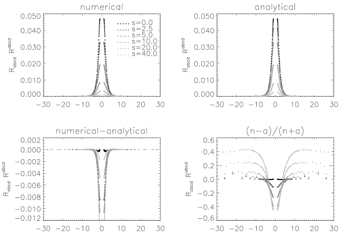
FIG. 5.: $I_{1}$ (eq. 17), as a function of isotropic coordinate y (which coincides with the equatorial axis) for rotating numerical and Kerr black holes.

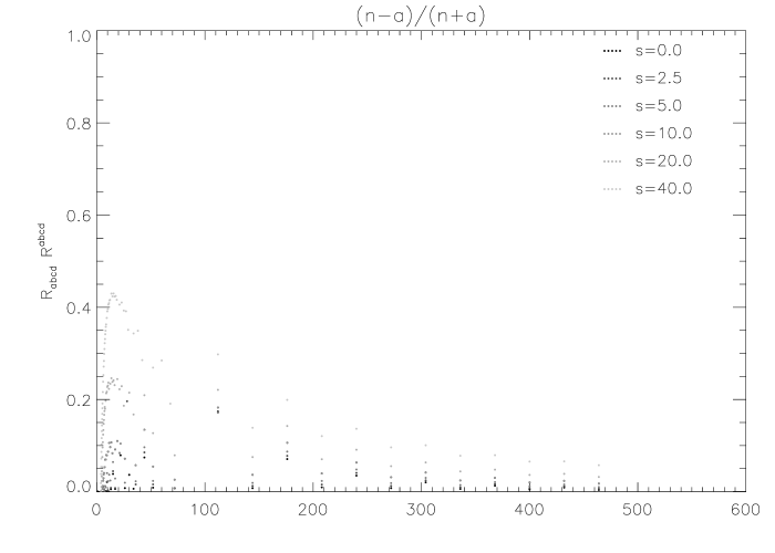
FIG. 6.: Relative comparison of $I_{1}$ (eq. 17) at large distances for rotating holes.

FIG. 7.: Asymptotic total mass, $M_{tot}$, and total linear momentum, $P_{tot}$, for case M=2 P=40. The diamonds are the numerical values of $M_{tot}$,$P_{tot}$ found from integrating over a sphere at radius $r$. The line is a least square fit of the data to a second order polynomial.

FIG. 8.: Total mass, $M_{tot}$, apparent horizon mass, $M_{ah}$, and boosted mass, $M_{boosted}$, as a function of P for a boosted black hole. $M_{tot}$ and $M_{ah}$ are calculated numerically, and $M_{boosted}=\sqrt{M_{tot}^{2}-P^{2}}$ is the horizon mass of a boosted Schwarzschild black hole with the same overall mass and linear momentum as the numerical black hole.

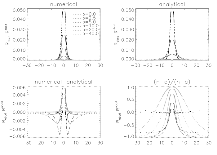
FIG. 9.: $I_{1}$ (eq. 17), as a function of isotropic coordinate x (which coincides with the equatorial axis) for moving numerical and boosted Schwarzschild black holes.

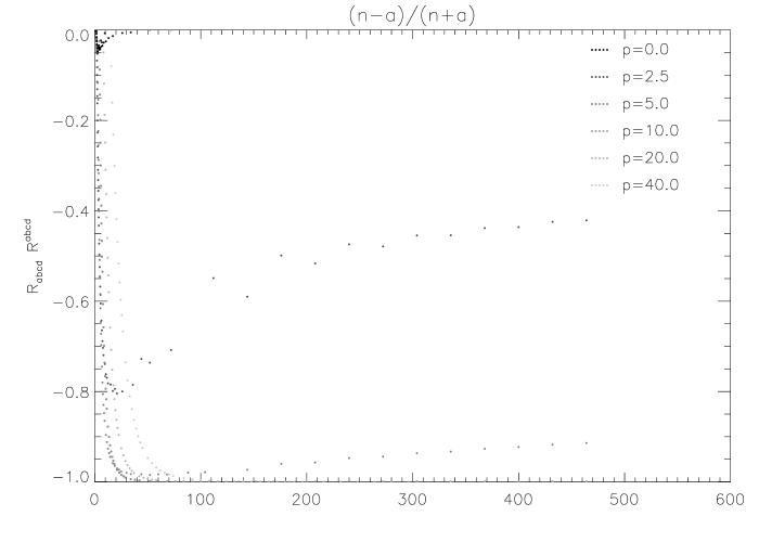
FIG. 10.: Relative comparison of $I_{1}$ (eq. 17) at large distances for boosted black holes.

A)

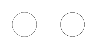
B)

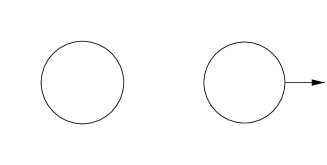
C)

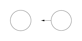
D)

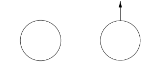
E)

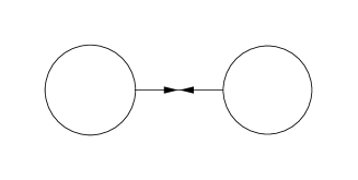
F)

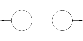
G)

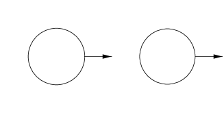
H)

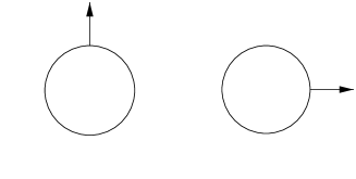
I)

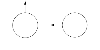
J)

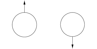
FIG. 11.: Schematic representation of 2 black hole configurations

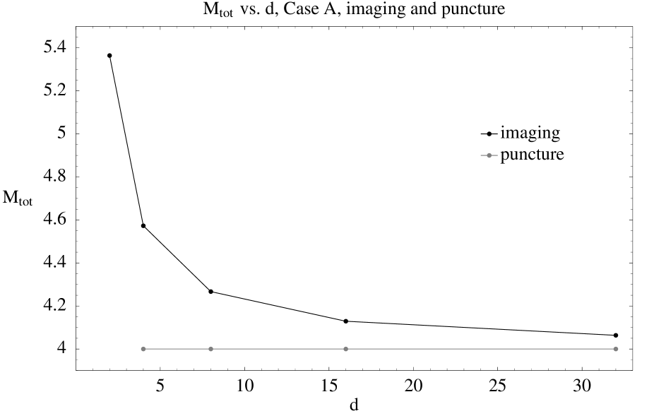
FIG. 12.: Total mass, $M_{tot}$ as a function of separation, $d$, for two black holes with configuration A (figure 11)

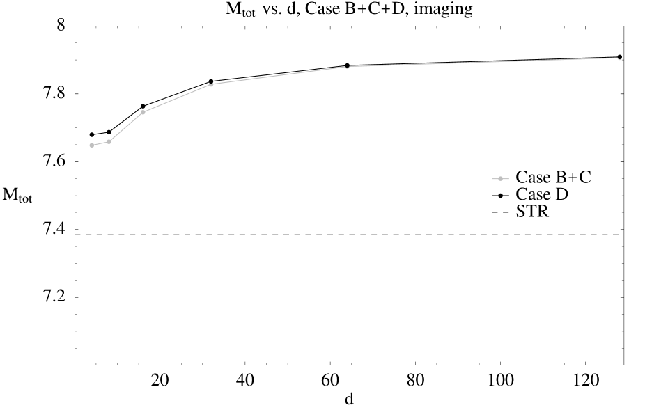
FIG. 13.: Total mass, $M_{tot}$, as a function of separation, $d$, for two black holes with configurations B, C, D (figure 11) with linear momentum, imaging method

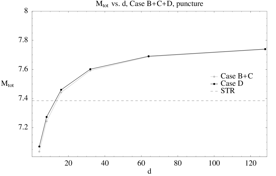
FIG. 14.: Total mass, $M_{tot}$, as a function of separation, $d$, for two black holes with configurations B, C, D (figure 11) with linear momentum, puncture method

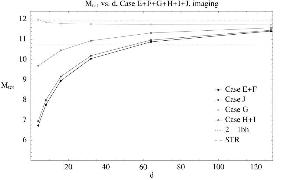
FIG. 15.: Total mass, $M_{tot}$, as a function of separation, $d$, for two black holes with configurations E, F, G, H, I, J (figure 11) with linear momentum, imaging method

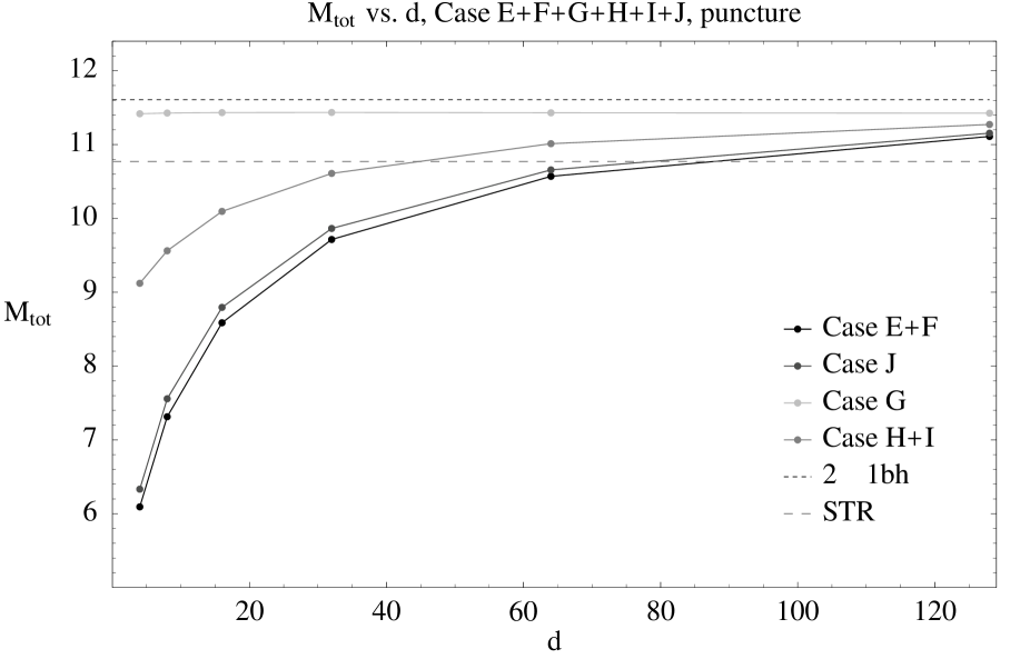
FIG. 16.: Total mass, $M_{tot}$, as a function of separation, $d$, for two black holes with configurations E, F, G, H, I, J (figure 11) with linear momentum, puncture method

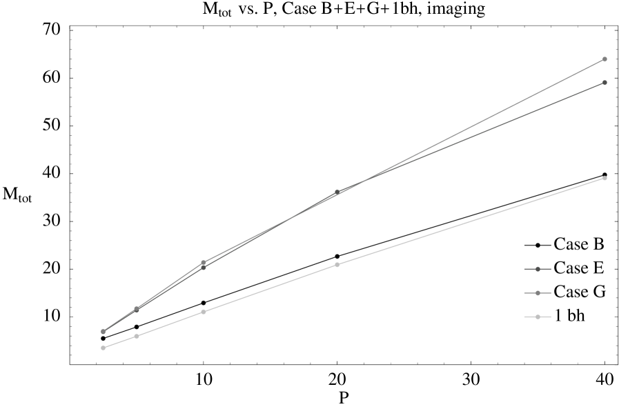
FIG. 17.: Total mass, $M_{tot}$ as a function of linear momentum, $P$, for separation $d=128$ for two black holes with configurations B, E, G (figure 11), imaging method

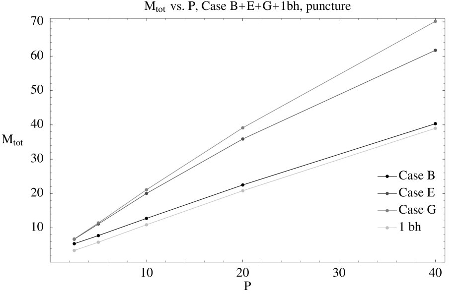
FIG. 18.: Total mass, $M_{tot}$ as a function of linear momentum, $P$, for separation $d=128$ for two black holes with configurations B, E, G (figure 11), puncture method

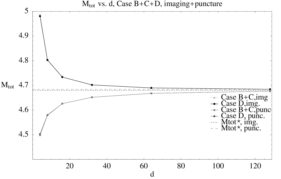
FIG. 19.: Total mass, $M_{tot}$, as a function of separation, $d$, for two black holes with configurations B, C, D (figure 11) with angular momentum

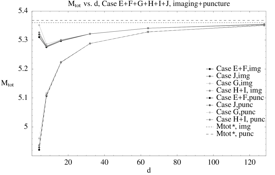
FIG. 20.: Total mass, $M_{tot}$, as a function of separation, $d$, for two black holes with configurations E, F, G, H, I, J (figure 11) with angular momentum

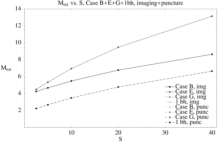
FIG. 21.: Total mass, $M_{tot}$ as a function of angular momentum, $S$, for separation $d=128$ for two black holes with configurations B, E, G (figure 11)

REFERENCES

- [1] Also at Copenhagen University Observatory, Denmark, NORDITA, Denmark and Astro Space Center of P.N. Lebedev Physical Institute, Russia
-
[2]
G.B. Cook, Living Reviews,
http://www.livingreviews.org/Articles/Volume3/2000-5cook/index.html - [3] J.M. Bowen and J.W. York, Jr., Phys. Rev. D 21, 2047 (1980).
- [4] J.W. York, Jr., J. Math. Phys. 14, 456 (1973).
- [5] J.W. York, Jr. and T. Piran, Spacetime and geometry, edited by R. Matzner and L. Shepley (University of Texas Press, Austin, 1982), pp. 147-176.
- [6] G.B. Cook, Phys. Rev. D44, 2983 (1991).
- [7] G.B. Cook, M.W. Choptuik, M.R. Dubal, S. Klasky, R.A. Matzner, and S.R. Oliveira, Phys. Rev. D47, 1471 (1993).
- [8] S. Brandt and Brgmann, Phys. Rev. Lett. 78, 3606 (1997).
- [9] P. Diener, N. Jansen, A. Khokhlov, I. Novikov, Class. Quantum Grav. 17 No 2 (21 January 2000) 435-451
- [10] L. D. Landau and E. M. Lifshitz. The Classical Theory of Fields. Butterworth-Heinemann Ltd.,1975.
- [11] A.M. Khokhlov, J. Comput. Phys. 143, 519 (1998)
- [12] James W. York, Jr. Kinematics and Dynamics of General Relativity. in: Sources of Gravitational Radiantion Editor Larry Smarr. Cambridge University Press, 1979.
- [13] G.B. Cook, Phys. Rev. D 50,5025,(1994)
- [14] G.B. Cook and J.W. York, Jr., Phys. Rev. D41, 1077 (1990).
- [15] L. Smarr, Phys. Rev. D7, 298, (1973)
- [16] C.W. Misner, Ann. Phys. (N.Y.) 24, 102 (1963).
A)
B)
C)
D)
E)
F)
G)
H)
I)
J)