Manufacture of Gowdy spacetimes with spikes

Abstract

In numerical studies of Gowdy spacetimes evidence has been found for the development of localized features (‘spikes’) involving large gradients near the singularity. The rigorous mathematical results available up to now did not cover this kind of situation. In this work we show the existence of large classes of Gowdy spacetimes exhibiting features of the kind discovered numerically. These spacetimes are constructed by applying certain transformations to previously known spacetimes without spikes. It is possible to control the behaviour of the Kretschmann scalar near the singularity in detail. This curvature invariant is found to blow up in a way which is non-uniform near the spike in some cases. When this happens it demonstrates that the spike is a geometrically invariant feature and not an artefact of the choice of variables used to parametrize the metric. We also identify another class of spikes which are artefacts. The spikes produced by our method are compared with the results of numerical and heuristic analyses of the same situation.

1 Introduction

The question of the nature of spacetime singularities in general relativity is far from being answered in general. The encouraging progress which has been made on this problem in the past few years has mainly consisted of obtaining detailed information about certain phenomena in more or less special classes of spacetimes. The effects which have been studied in a rigorous mathematical way include the decoupling of the evolution at different spatial points near the singularity (see [1], [17], [19] and references therein) and the monotone or oscillatory approach to the singularity, which has been investigated in the case of spatially homogeneous spacetimes ([24], [22], [23], [20], [21]). In numerical work it has been possible to study both together ([7], [25], [9]). The first of these effects means that an inhomogeneous model can be approximated near the singularity by a family of homogeneous models parametrized by the spatial coordinates and this is why the second is of wider importance. This choice of topics was stimulated by the pioneering ideas of Belinskii, Khalatnikov and Lifshitz (BKL) (see [4] and references therein).

One class of spacetimes which has turned out to be particularly useful in developing ideas about the nature of spacetime singularities is that of Gowdy spacetimes. These do not show an infinite number of oscillations as the singularity is approached in the way that generic spacetimes are supposed to do according to the BKL picture. Instead they appear to show a monotone behaviour near the singularity which is called velocity dominated ([13], [16]). Thus they provide a relatively simple arena for studying spacetime singularities. On the other hand, as will become clear in the following, the Gowdy spacetimes do display quite complicated dynamical behaviour near their initial singularities and it is probable that what we can learn from them will be useful in understanding more general classes of spacetimes.

The Gowdy spacetimes which have been studied most extensively are those with spatial topology $T^{3}$ and only these will be discussed in the following. Grubišić and Moncrief [14] derived a consistent formal expansion for Gowdy spacetimes near their singularities under a certain assumption. For Gowdy spacetimes it is possible to consider a quantity $v$ called the velocity. (Since $v$ is a non-negative scalar quantity it would be more appropriate to call it speed, but we will retain the usual terminology.) If velocity dominance holds this quantity has a (space-dependent) limit as the singularity is approached. It is also possible to associate a sign to each spatial point and thus define a real-valued function $k$ with the given magnitude and sign. This function will be called the asymptotic velocity. The Grubišić-Moncrief expansion is consistent provided $0<k<1$, which defines what is called the low velocity regime. For high velocity ($k\geq 1$) this is no longer true in general. (Some remarks on the meaning of $k\leq 0$ will be made later.) It was suggested in [14] that in those cases where the expansion is not consistent the solution evolves in such a way that the velocity is eventually less than one close to the singularity. It was also noticed that under an additional non-generic condition it is possible for the expansion to be consistent with high velocity.

A little later Berger and Moncrief [8] observed the development of large spatial derivatives near the singularity in numerical calculations of Gowdy spacetimes. They called these ‘spiky features’. We will abbreviate this to ‘spikes’. They presented evidence that these were genuine features of the spacetimes and not numerical artifacts. Spikes were seen to be associated with the situation where the non-generic condition of [14] is satisfied at an isolated point. In this case it can happen that the velocity stays high at the special point as the singularity is approached while it is forced below one everywhere else. This gives an intuitive picture of how under certain circumstances strongly spatially inhomogeneous behaviour may develop in Gowdy spacetimes as the singularity is approached.

In the special case of the polarized Gowdy spacetimes velocity dominance has been proved [16]. There is also a theorem on the structure of the initial singularity in those non-polarized vacuum models evolving from data which are close to those for a particular Kasner solution (with exponents $\frac{2}{3},\frac{2}{3},-\frac{1}{3}$) [12]. The model solution has velocity $v$ identically zero. The discovery of spikes in the evolution of general Gowdy models implies limits to the way in which these results for particular subclasses could generalize.

A complementary development to these theorems on the nature of the singularity arising from given Cauchy data for a Gowdy spacetime is the construction of large classes of solutions with singularities of a particular type. This was carried out for the case of velocity dominated singularities with asymptotic velocity satisfying $0<k<1$ by Kichenassamy and Rendall [17]. Solutions were constructed depending on four free functions, which is the same number as in the general solution. Intuitively this suggests that solutions corresponding to an open set of initial data are being obtained by this procedure, although it has not been possible to prove this yet. Solutions depending on three free functions were also constructed under the weaker restriction $k>0$. In [17] the free functions were required to be analytic, but this undesirable restriction was removed in [19]. In the following the low velocity solutions of [17] and [19] will be used as a starting point to produce another family of solutions, depending on the same number of free functions, which exhibit spikes.

If one looks at numerically produced spikes (see e.g. figure 2 in [5]) then it becomes clear that there are two different types and that within any one of these types the individual spikes show a great similarity among themselves. This is a strong motivation for finding a simple explanation, and the main result of this paper is to do this in a mathematically rigorous way. The principal unknowns in the Einstein equations for Gowdy metrics are real-valued functions $P$ and $Q$. In one case $P$ has a spike and $Q$ has a kind of discontinuity while in the other case $P$ has a spike of the same shape but pointing in the opposite direction while $Q$ is smooth. For reasons to be explained later, these will be called ‘false’ and ‘true’ spikes, respectively. A key feature is that in the first case geometric quantities such as curvature invariants show no irregular behaviour at the spike as the singularity is approached, while in the second case they do.

The field equations in Gowdy spacetimes are known to be closely related to the geometry of the hyperbolic plane (see, for instance, [14]). The interpretation in terms of hyperbolic geometry leads rather easily to a transformation (inversion) which produces solutions with false spikes from the smooth low velocity solutions of [17]. More subtle is a further transformation (Gowdy-to-Ernst transformation) which converts solutions with false spikes into solutions with true spikes. It is related to the Kramer-Neugebauer transformation ([18], [10]) occurring in the theory of stationary and axisymmetric spacetimes.

The paper is organized as follows. In section 2 the basic notations and equations are introduced and the two transformations of key importance in the following are defined. The third section introduces the concepts of false and true spikes, shows how solutions displaying features of this kind can be produced and gives asymptotic expansions for these solutions near the spikes. In the fourth section the analytical and numerical results are compared. Section 5 relates what we have found here to the method of consistent potentials and hence to the dynamics which produces these solutions. Finally, section 6 discusses some further developments of the results.

2 The Gowdy spacetimes

The Gowdy spacetimes on $T^{3}$ are solutions of the vacuum Einstein equations which can be written in the form

$$g=-e^{(\lambda-3\tau)/2}d\tau^{2}+e^{(\lambda+\tau)/2}dx^{2}+e^{P-\tau}(dy+Q\,dz)^{2}+e^{-P-\tau}dz^{2}$$ (1)

They admit $U(1)\times U(1)$ as an isometry group, acting by translation of the periodic coordinates $y$ and $z$. The notation here differs somewhat from that used in [17]. The quantities $(P,Q,\tau)$ occurring here are related to the quantities $(X,Z,t)$ of [17] by

$$t=e^{-\tau}\hskip 20.0ptP=-Z\hskip 20.0ptQ=X$$

The coordinate $t$, and hence the coodinate $\tau$, is determined in an invariant way by the geometry: $t$ is proportional to the area of the the orbits of the symmetry group. The functions $P$ and $Q$ depend on $\tau$ and $x$. For a Gowdy spacetime on $T^{3}$ they should be periodic in $x$, but most of this paper is concerned with constructions which are local in $x$. Information about the initial singularity, which is at $t=0$, is encoded here in the asymptotic behaviour of the metric as $\tau\to\infty$. The vacuum Einstein equations imply that the functions $P$ and $Q$ satisfy

$$P_{\tau\tau} = e^{2P}Q_{\tau}^{2}+e^{-2\tau}(P_{xx}-e^{2P}Q_{x}^{2})$$

$$Q_{\tau\tau} = -2P_{\tau}Q_{\tau}+e^{-2\tau}(Q_{xx}+2P_{x}Q_{x})$$ (2)

and that $\lambda$ satisfies

$$\lambda_{\tau} = -(P_{\tau}^{2}+e^{2P}Q_{\tau}^{2})-e^{-2\tau}(P_{x}^{2}+e^{2P}Q_{x}^{2})$$

$$\lambda_{x} = -2(P_{\tau}P_{x}+e^{2P}Q_{\tau}Q_{x})$$ (3)

These equations determine $\lambda$ up to a constant. When the above equations are satisfied $P$, $Q$ and $\lambda$ define a solution of the vacuum Einstein equations via (1).

Suppose that a solution $(P_{0},Q_{0})$ of (2) is given. Define functions $(P_{1},Q_{1})=I(P_{0},Q_{0})$ by

$$e^{-P_{1}}={e^{-P_{0}}\over Q_{0}^{2}+e^{-2P_{0}}}\hskip 40.0ptQ_{1}={Q_{0}\over Q_{0}^{2}+e^{-2P_{0}}}$$ (4)

Then $(P_{1},Q_{1})$ also satisfy (2), as can be checked by direct calculation. The transformation $(P_{0},Q_{0})\stackrel{{\scriptstyle I}}{{\longrightarrow}}(P_{1},Q_{1})$ has been denoted by $I$, since it has a geometric interpretation in terms of an inversion in the hyperbolic plane. This will now be explained in some detail.

The description of Gowdy spacetimes in terms of the three real-valued functions $P$, $Q$ and $\lambda$ of $\tau$ and $x$ can be replaced by one with greater invariance which leads to useful insights. For this purpose it is useful to think of these as functions of $t$ and $x$ which, with a slight abuse of notation, will be denoted by the same letters. Let $M$ be the manifold with coordinates $t$ and $x$, which is just an open subset of ${\bf R}^{2}$. Let the flat metric $-dt^{2}+dx^{2}$ on $M$ be denoted by $f$. Define a mapping from $M$ to ${\bf R}^{2}$ by the pair $U=(P,Q)$. Let $(N,h)$ be ${\bf R}^{2}$ with the metric $h$ defined by $dP^{2}+e^{2P}dQ^{2}$. The derivative $dU$ is a section of the tensor product of the cotangent bundle of $M$ with the pull-back via $U$ of the tangent bundle of $N$ to $M$. There is a natural connection defined on this bundle by means of the Levi-Civita connections associated to the metrics $f$ and $h$. This defines a covariant derivative, call it $D$. The Gowdy equations for $P$ and $Q$ take the form ${\rm tr}_{f}(DdU)-t^{-1}U_{t}=0$. This a slight generalization of the equation for a wave map (also known as a hyperbolic harmonic map or nonlinear $\sigma$-model) which is ${\rm tr}_{f}(DdU)=0$. The functions of $P$ and $Q$ occurring in the equations for $\lambda$ are also expressible in terms of $h$. They are just $h(U_{t},U_{t})+h(U_{x},U_{x})$ and $h(U_{t},U_{x})$. It follows that all the Gowdy field equations can be expressed in a way which is covariant with respect to $(N,h)$. An advantage of this is that applying any isometry of $h$ to a solution of the Gowdy equations will give a new solution. It can be shown that the metric corresponding to the functions $(P,Q,\lambda)$ after transformation is isometric to the original one, the transformation being effected by a linear change of the variables $y$ and $z$. This will not be proved here, since we only need it in one special case (inversion), where it can be checked directly. The fact that the two metrics are isometric means that quantities such as invariants of the spacetime curvature are identical for the original solution and the transformed solution.

Another way of looking at the invariance properties of the equations and their relation to wave maps is via a Lagrangian formulation. A wave map from two-dimensional Minkowski space to the hyperbolic plane is the Euler-Lagrange equation corresponding to the action

$$\int f^{ij}\partial_{i}U^{A}\partial_{j}U^{B}h_{AB}dV(f)$$ (5)

$$= \int((-P_{t}^{2}+P_{x}^{2})+e^{2P}(-Q_{t}^{2}+Q_{x}^{2}))dtdx$$

The Gowdy equations are the Euler-Lagrange equations for the analogous action

$$\int((-P_{\tau}^{2}+e^{-2\tau}P_{x}^{2})+e^{2P}(-Q_{\tau}^{2}+e^{-2\tau}Q_{x}^{2}))d\tau dx$$ (6)

One isometry of the metric $h$ is given by the transformation (4). This was written down in a slightly different notation in [17]. Its geometrical origin is as follows. Define $Y=e^{-P}$. The metric $h$ is that of hyperbolic space and the coordinates $(Q,Y)$ give the well-known upper half-space representation of that space on the region $Y>0$. In that representation the transformation introduced above becomes inversion in the unit circle and it interchanges the origin with the point at infinity. For this reason this transformation is referred to as inversion $I$ in the following. It is induced by the linear transformation of coordinates which interchanges $y$ and $z$. Another representation of the hyperbolic space is given by the Poincaré disk model, where the points of the boundary of the half-space model are all on an equal footing with the point at infinity. From this point of view it is clear that the coordinates $(P,Q)$ break the symmetry of the hyperbolic plane by singling out a point of its ideal boundary as the point at infinity. The inversion $I$ changes this choice.

Next another transformation which generates new solutions from old will be introduced. We know of no simple geometric interpretation such as that given for $I$ above. In contrast to $I$, which transforms one coordinate representation of a metric into another representation of the same metric, the transformation which will be considered now produces a genuinely new metric (i.e. one which is not isometric to the original one). This transformation was suggested by the fact, already discussed in detail in [11], that a given Gowdy spacetime defines two pairs of functions which satisfy identical equations. These come from the Gowdy and Ernst methods of reduction with respect to the Killing vectors of the spacetime and so we will call this transformation GE for Gowdy-to-Ernst. If $(P_{1},Q_{1})$ is a solution of the Gowdy equations then the transformation $(P_{1},Q_{1})\stackrel{{\scriptstyle GE}}{{\longrightarrow}}(P_{2},Q_{2})$ is defined by

$$P_{2}=-P_{1}+\tau\hskip 20.0ptQ_{2\tau}=-e^{2(P_{1}-\tau)}Q_{1x}\hskip 20.0ptQ_{2x}=-e^{2P_{1}}Q_{1\tau}$$ (7)

In fact, $Q_{2}$ is only defined up to an additive constant by these relations and it is necessary to be careful about specifying the constant when applying the transformation for a specific purpose. The integrability condition only assures the existence of a solution locally in $x$ and in most of this paper we will restrict to that situation. See, however, the comments on spikes in (global) Gowdy spacetimes in section 6. The transformation $GE$ is such that if $(P_{1},Q_{1})$ satisfy the Gowdy equations (2) then $(P_{2},Q_{2})$ do so too. That the integrability condition for $Q_{2\tau}$ and $Q_{2x}$ is satisfied can be verified directly by calculating the $x$-derivative of the right hand side of the expression for $Q_{2\tau}$ and the $\tau$-derivative of the right hand side of the expression for $Q_{2x}$ and seeing that they agree if $P_{1}$ and $Q_{1}$ satisfy the Gowdy equations. There is a close relationship between this transformation and the Kramer-Neugebauer transformation for stationary axisymmetric spacetimes (see [18], [10]). They differ by no more than signs related to the different character of the Killing vectors (both spacelike in the one case, one timelike and one spacelike in the other case).

Since the relations (7) only fix $Q_{2}$ up to a constant, there is in fact a whole one-parameter family of solutions produced by this procedure which differ by translations in the $Q$-direction. On the other hand, changing $Q_{1}$ by a constant does not change $Q_{2}$.

3 Construction of solutions with spikes

The central procedure of this paper is the manufacture of solutions of the Gowdy equations with spikes out of solutions without spikes by means of the transformations $I$ and GE introduced in the last section. The source of solutions without spikes which we draw on is a class of solutions constructed in [19] and so we begin by describing those solutions in terms of the variables used here. Let $\epsilon$ be a positive constant and let $k(x)$, $X_{0}(x)$, $\phi(x)$ and $\psi(x)$ be periodic $C^{\infty}$ functions, i.e. smooth functions defined on $S^{1}$. Suppose that $\epsilon<2k(x)$, $\epsilon<2(1-k(x))$ and $0<k(x)<1$. Then there exist unique $C^{\infty}$ functions $u(\tau,x)$ and $v(\tau,x)$, periodic in $x$, which converge to zero in the limit that $\tau\rightarrow\infty$ such that the functions $P(\tau,x)$ and $Q(\tau,x)$,

$$P=k\tau-\varphi-e^{-\epsilon\tau}\,u\hskip 40.0ptQ=X_{0}+e^{-2k\tau}\,(\psi+v)$$ (8)

satisfy the equations (2). A similar statement holds locally. If the input functions $k$, $X_{0}$, $\phi$ and $\psi$ are defined for $x$ belonging to some open interval, then a unique solution as above is obtained for $x$ belonging to some slightly smaller open interval. The function $k$ coincides with the asymptotic velocity mentioned in the introduction and is positive in this case. Note that statements of this kind were originally proved in [17] under the additional hypothesis of analyticity of the input functions. We will refer to these solutions (whether analytic or not) as the low velocity KR (Kichenassamy-Rendall) solutions.

It follows from what has been said about $P$ and $Q$ above that

$$P=k\tau-\varphi+o(1)\hskip 40.0ptQ=X_{0}+e^{-2k\tau}\,\psi+o(e^{-2k\tau})$$ (9)

It is also important for the following to know that these asymptotic expansions can be differentiated term by term in an appropriate sense. This is a consequence of the fact that the functions $u$ and $v$ are regular in the sense of Definition 1 in [19]. It can be concluded that

$$\partial_{x}^{j}P=\partial_{x}^{j}k\tau-\partial_{x}^{j}\varphi+o(1)$$ (10)

for all $j\geq 0$. For $Q$ we have the slightly more complicated statement that

$$\partial_{x}^{j}Q=\partial_{x}^{j}X_{0}+\partial_{x}^{j}(e^{-2k\tau}\,\psi)+o(\tau^{j}e^{-2k\tau})$$ (11)

In this relation it is also possible to replace $\partial_{x}^{j}(e^{-2k\tau}\psi)$ by $\partial_{x}^{j}k(-2\tau)^{j}e^{-2k\tau}\psi$. Estimates for time derivatives can be obtained by substituting these expressions into equations (2). (To be precise, this is true for time derivatives of order at least two. The statements for the first order time derivatives are direct consequences of the theorems of [19], which were proved using a first order formulation of the equations, where the time derivatives of the basic variables are included as unknowns.) There results the estimate

$$\partial_{\tau}^{l}\partial_{x}^{j}P=\partial_{\tau}^{l}\partial_{x}^{j}(k\tau)+o(1)$$ (12)

for all $j\geq 0$ and $l>0$. Of course the first term on the right hand side vanishes as soon as $l>1$. Similarly

$$\partial_{\tau}^{l}\partial_{x}^{j}Q=\partial_{\tau}^{l}\partial_{x}^{j}(e^{-2k\tau}\,\psi)+o(\tau^{j}e^{-2k\tau})$$ (13)

Consider now a low velocity KR solution $(P_{0},Q_{0})$ such that the corresponding function $X_{0}$ vanishes at an isolated point $x_{spike}$. Applying the transformation $I$ produces a new solution $(P_{1},Q_{1})$ of the Gowdy equations according to equations (4). The intuitive idea is that the new solution has a spike at $x_{spike}$, a statement which will be made precise later. Applying the transformation $I$ to (8) with $(P,Q)$ replaced by $(P_{0},Q_{0})$, one finds that

$$P_{1} = k\tau-\varphi-e^{-\epsilon\tau}u+\ln\{[X_{0}+e^{-2k\tau}(\psi+v)]^{2}+e^{-2k\tau}e^{2\varphi}e^{2e^{-\epsilon\tau}u}\}$$

$$Q_{1} = {X_{0}+e^{-2k\tau}(\psi+v)\over[X_{0}+e^{-2k\tau}(\psi+v)]^{2}+e^{-2k\tau}e^{2\varphi}e^{2e^{-\epsilon\tau}u}}$$ (14)

The aim now is to investigate the qualitative behaviour of this solution in the limit $\tau\to\infty$. This will be done by fixing a point $x$ and expanding in $\tau$ in a suitable way. It turns out that the result is quite different depending whether $x$ is equal to $x_{spike}$ or not. At $x_{spike}$ one finds that

$$P_{1} = -k\tau+\varphi+e^{-\epsilon\tau}\tilde{u}_{a}$$

$$Q_{1} = e^{-2\varphi}(\psi+v)+e^{-\epsilon\tau}\tilde{v}_{a}$$ (15)

for some functions $\tilde{u}_{a}$ and $\tilde{v}_{a}$ with $\lim_{\tau\rightarrow\infty}\tilde{u}_{a}=0$ and $\lim_{\tau\rightarrow\infty}\tilde{v}_{a}=0$. Elsewhere one finds that

$$P_{1} = k\tau-\varphi+\ln X_{0}^{2}+e^{-\epsilon\tau}\tilde{u}_{b}$$

$$Q_{1} = {1\over X_{0}}+e^{-2k\tau}(-{\psi\over X_{0}^{2}}-{e^{2\varphi}\over X_{0}^{3}}+\tilde{v}_{b})$$ (16)

for some functions $\tilde{u}_{b}$ and $\tilde{v}_{b}$ with $\lim_{\tau\rightarrow\infty}\tilde{u}_{b}=0$ and $\lim_{\tau\rightarrow\infty}\tilde{v}_{b}=0$. At each spatial point the asymptotic behaviour in time is of a similar form to that of the KR solutions. However the coefficients of the leading terms behave in a very non-uniform way as a function of $x$ close to the spike. The coefficient corresponding to $k(x)$, the asymptotic velocity, has a discontinuity at $x_{spike}$ while the coefficient corresponding to $X_{0}$ is unbounded near that point. This means that the spatial derivatives of the functions $P$ and $Q$ close to the point $x_{spike}$ grow much faster as $\tau\to\infty$ than is the case for the KR solutions. This behaviour shows up as spikes in numerical calculations. Since it is obviously an effect of the parametrization of the metric and not a geometrical one, we refer to this kind of point as a ‘false spike’. Note that at a false spike the asymptotic velocity is negative. This shows that the sign of $k$ has no absolute geometric significance in general.

Applying the transformation GE to $(P_{1},Q_{1})$ gives a new solution $(P_{2},Q_{2})$. It also has a spike at the point $x_{spike}$ and, as will be proved later, curvature invariants show highly non-uniform behaviour there. This shows in particular that in this case there has been a change in the geometry and so we refer to this kind of point as a ‘true spike’. In this case one finds that

$$P_{2} = (1-k)\tau+\varphi+e^{-\epsilon\tau}u-\ln\{[X_{0}+e^{-2k\tau}(\psi+v)]^{2}+e^{-2k\tau}e^{2\varphi}e^{2e^{-\epsilon\tau}u}\}$$

$$Q_{2\tau} = e^{-2\tau}\{-X_{0x}-e^{-2k\tau}(\psi_{x}+v_{x})+$$

$$[e^{2k\tau}X_{0x}+\psi_{x}+v_{x}-2k_{x}\tau(\psi+v)][X_{0}+e^{-2k\tau}(\psi+v)]^{2}e^{-2\varphi}e^{-2e^{-\epsilon\tau}u}$$

$$-2k_{x}\tau X_{0}+2[X_{0}+e^{-2k\tau}(\psi+v)][\varphi_{x}+e^{-\epsilon\tau}u_{x}]\}$$

$$Q_{2x} = -e^{-2k\tau}v_{\tau}+(-2k(\psi+v)+v_{\tau})[X_{0}+e^{-2k\tau}(\psi+v)]^{2}e^{-2\varphi}e^{-2e^{-\epsilon\tau}u}$$ (17)

$$-2kX_{0}+2X_{0}e^{-\epsilon\tau}(u_{\tau}-\epsilon u)+2e^{-(2k+\epsilon)\tau}(\psi+v)(u_{\tau}-\epsilon u)$$

At $x_{spike}$ one finds that

$$P_{2} = (1+k)\tau-\varphi+e^{-\epsilon\tau}\tilde{u}_{c}$$

$$Q_{2\tau} = -e^{-2\tau}X_{0x}+e^{-2(1+k)\tau}(-\psi_{x}+X_{0x}\psi^{2}e^{-2\varphi}+2\psi\varphi_{x}+\hat{v}_{c})$$

$$Q_{2x} = -e^{-2k\tau}v_{\tau}+2e^{-(2k+\epsilon)\tau}(\psi+v)(u_{\tau}-\epsilon u)$$ (18)

$$-2ke^{-4k\tau}\psi^{3}e^{-2\varphi}+e^{-4k\tau}\check{v}_{c}$$

with $\lim_{\tau\rightarrow\infty}\tilde{u}_{c}=0$, $\lim_{\tau\rightarrow\infty}\hat{v}_{c}=0$ and $\lim_{\tau\rightarrow\infty}\check{v}_{c}=0$. Elsewhere one finds that

$$P_{2} = (1-k)\tau+\varphi-\ln X_{0}^{2}+e^{-\epsilon\tau}\tilde{u}_{d}$$

$$Q_{2\tau} = e^{-2(1-k)\tau}X_{0}^{2}X_{0x}e^{-2\varphi}e^{-2e^{-\epsilon\tau}u}+e^{-2\tau}\{-X_{0x}+2X_{0}X_{0x}\psi e^{-2\varphi}$$ (19)

$$+X_{0}^{2}(\psi_{x}-2k_{x}\tau\psi)e^{-2\varphi}-2k_{x}\tau X_{0}+2X_{0}\varphi_{x}+\hat{v}_{d}\}$$

$$Q_{2x} = -2kX_{0}+(-2k(\psi+v)+v_{\tau})X_{0}^{2}e^{-2\varphi}e^{-2e^{-\epsilon\tau}u}$$ (20)

$$-4ke^{-2k\tau}\psi^{2}X_{0}e^{-2\varphi}+2X_{0}e^{-\epsilon\tau}(u_{\tau}-\epsilon u)+e^{-2k\tau}\check{v}_{d}$$

with $\lim_{\tau\rightarrow\infty}\tilde{u}_{d}=0$, $\lim_{\tau\rightarrow\infty}\hat{v}_{d}=0$ and $\lim_{\tau\rightarrow\infty}\check{v}_{d}=0$.

While the pointwise expansions which have been obtained so far contain much valuable information, it is also useful to derive uniform expansions of the solutions on suitable regions. This will only be done for the true spikes, which are the main focus of interest here. For a true spike $Q_{2}$ behaves in a regular way and so the point $x_{spike}$ does not have to be considered separately. It is possible to get a uniform asymptotic expansion for $\tau$ large and $x$ in a neighbourhood of $x_{spike}$. The expansions for $P$ and $Q$ and their derivatives imply corresponding expansions for $Q_{2\tau}$, $Q_{2x}$ and their derivatives. An expansion for $Q_{2}$ itself can be obtained straightforwardly by integration. All these expansions are of the same form as those of the starting low velocity solution.

In the case of $P_{2}$ it is necessary to distinguish between two different regions in order to get uniform expansions. Let $k_{*}$ be a positive number. The interesting case is where $k_{*}$ is slightly greater or slightly less than the value of $k$ at $x_{spike}$, and hence has the same property for $x$ close to $x_{spike}$. Let $\sigma(\tau,x)=e^{k_{*}\tau}|x-x_{spike}|$. Intuitively the function $\sigma$ is a measure of the relative influence of the spike and the part of the boundary with low velocity asymptotics. We will see that the spike dominates when $\sigma$ is small while the low velocity behaviour dominates when $\sigma$ is large.

For convenience of notation, let $\delta x=|x-x_{spike}|$. Consider a region $R_{1}$ where $\tau$ is sufficiently large, $\delta x$ sufficiently small and $\sigma\geq 1$. We also make the genericity assumption that $|X_{0x}(x_{spike})|=\eta>0$. Given $0<\alpha<1$ it can be assumed by choosing $R_{1}$ to make $\delta x$ sufficiently small, that on the region $R_{1}$ we have $|X_{0}|\geq\alpha\eta\delta x$ and

$$|X_{0}|^{-1}\leq\alpha^{-1}\eta^{-1}e^{k_{*}\tau}$$ (21)

Now choose $k_{*}<k(x_{spike})$. Then

$$[X_{0}+e^{-2k\tau}(\psi+v)]^{2}+e^{-2k\tau}e^{2\phi}e^{2e^{-\epsilon\tau}u}=X_{0}^{2}[1+O(e^{-2(k-k_{*})\tau})]$$ (22)

The logarithm of this expression is then equal to the logarithm of $X_{0}^{2}$ up to a remainder of which is $O(e^{-2(k-k_{*})\tau})$. In this way it can be seen that $P_{2}$ has an expansion on the region $R_{1}$ which is of the same form as that for the starting function $P$. In particular this expansion can be differentiated term by term.

Next consider a region $R_{2}$ where $\tau$ is sufficiently large, $\delta$ is sufficiently small and $\sigma\leq 1$. Then we can carry out a very similar procedure. This time we choose an arbitrary $\alpha>1$ and $k_{*}>k(x_{spike})$. It is convenient to rewrite the expression for $P_{2}$ as

$$P_{2}=(1+k)\tau-\varphi-e^{-\epsilon\tau}u-\ln\{1+[e^{k\tau}X_{0}+e^{-k\tau}(\psi+v)]^{2}e^{-2\varphi}e^{-2e^{-\epsilon\tau}u}\}$$ (23)

On the region $R_{2}$ an estimate of the form $e^{k\tau}|X_{0}|\leq\alpha\eta e^{(k-k_{*})\tau}$ holds. Thus the logarithm in the last expression for $P_{2}$ is $O(e^{2(k-k_{*})\tau})$ on $R_{2}$. We obtain a uniform asymptotic expansion for the solution on the region $R_{2}$ which can be differentiated term by term. This expansion is of the same form as those for high velocity KR solutions.

The significance of the above observations concerning uniform asymptotic expansions is that in order to determine the behaviour of curvature invariants in the regions $R_{1}$ and $R_{2}$ it is sufficient to use the expressions already derived in [17], since all the assumptions needed to do that computation are also satisfied on the regions $R_{1}$ and $R_{2}$ in the present case, although for rather different reasons. In particular the information about what happens as a point of the boundary is approached with $x$ a constant other than $x_{spike}$ can be read off from the asymptotics in the region $R_{1}$ while the information about what happens when the boundary is approached along $x=x_{spike}$ is given by the asymptotics in the region $R_{2}$. It follows that the Kretschmann scalar $K=R^{\alpha\beta\gamma\delta}R_{\alpha\beta\gamma\delta}$ is given up to terms of lower order by $K=t^{-(\hat{k}^{2}+3)}B(\hat{k})$ where $B(\hat{k})=64(\hat{k}-1)^{2}(\hat{k}+1)^{2}(\hat{k}^{2}+3)^{-3}$ and $\hat{k}$ is the asymptotic velocity at the given value of $x$. For $x\neq x_{spike}$ this is $\hat{k}=1-k(x)$ while $\hat{k}(x_{spike})=1+k(x_{spike})$. For the solutions under consideration $B(\hat{k})$ never vanishes. Thus the Kretschmann scalar blows up like a more negative power of the Gowdy time $t$ at the spike than elsewhere. Since the Gowdy time is fixed invariantly by the spacetime geometry, this provides clear evidence that the non-uniformity near a true spike is a feature of the geometry and cannot be removed by a reparametrization as can be done in the case of the false spike. Note that there is a uniform lower bound for the rate of blow-up of $K$ in a neighbourhood of the spike and so there can be no violation of cosmic censorship there.

The mean curvature blows up like $t^{-(\hat{k}^{2}+3)/4}$. This shows that the singularity is a crushing singularity even in the presence of a true spike. If the Kretschmann scalar is expressed in terms of the mean curvature then the same power is obtained everywhere. However the constant of proportionality changes discontinuously as a function of $x$ as the spike is passed.

In [15] Hern investigated the behaviour of curvature invariants in dynamical numerical calculations of Gowdy spacetimes. Our results are consistent with his and in some cases help to explain them. He investigated more invariants and more aspects of their behaviour than we have done. The approach used here should also suffice to obtain more detailed information about more curvature invariants in the spikes we manufacture, if desired.

4 Comparison with numerical results

In the previous section we produced solutions of the Gowdy equations where the functions $P$ and $Q$ behave in an inhomogeneous way near the initial singularity. The motivation for this was to provide an explanation and rigorous confirmation of various features which had been observed in numerical calculations. In this section the analytical and numerical results will be compared so as to show their similarities.

As already mentioned in the introduction, looking directly at the results of the numerical calculations leads to the conclusion that near the singularity, and for generic initial data, there are a finite number of points where $P$ has a spike and that these points can be classified into two types according to whether the spike in $P$ points upwards or downwards and whether $Q$ is smooth or also exhibits inhomogeneous behaviour. We claim that the ‘false’ and ‘true’ spikes constructed in section 3 reproduce the qualitative features observed numerically.

Consider first false spikes. The coefficient of the leading term in the expansion of the function $P_{1}$ has a discontinuous limit at the singularity. The asymptotic velocity jumps. At the spike it is between $0$ and $-1$. At fixed time we see the influence of the expression $2X_{0}$ a little away from the spike. Under the generic assumption that $X_{0x}(x_{spike})\neq 0$ this behaves like a constant times $\log|x-x_{spike}|$ and accounts for the shape of the flanks of the spike. The spike points downwards. The coefficient of the leading term in the expansion for $Q_{1}$ is unbounded near the spike and at fixed time behaves like a constant times $(x-x_{spike})^{-1}$ (assuming the genericity condition). This leads to a growing jump in $Q$ between positive and negative values as the singularity is approached. Another quantity which has been studied numerically is the momentum conjugate to $Q$ in a Hamiltonian formulation, $\pi_{Q}=e^{2P}Q_{\tau}$. Calculation of $\pi_{Q1}$ from $P_{1}$ and $Q_{1}$ shows that it tends to zero as $t\to 0$ at $x_{spike}$. These features are observed in numerical calculations of the dynamics. To compare the two, we present pictures of the results of applying the transformation $I$ to a low velocity KR solution in figures 1–3. For purpose of illustration we choose periodic functions (with period $2\pi$) for $k$, $X_{0}$, $\varphi$ and $\psi$, and ignore the decaying unknowns $u$ and $v$. The salient features of the spikes do not depend on the particular form of the data, but to obtain a spike $X_{0}$ must vanish at an isolated point.

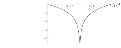
Figure 1: $P_{1}$ in a neighbourhood of $x_{spike}$ at small $t$.

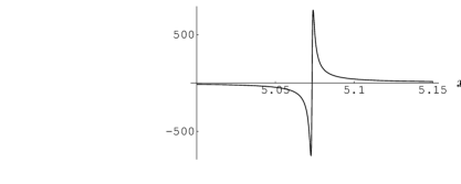
Figure 2: $Q_{1}$ in a neighbourhood of $x_{spike}$ at small $t$.

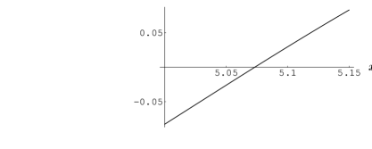
Figure 3: $\pi_{Q1}$ in a neighbourhood of $x_{spike}$ at small $t$.

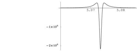
Figure 4: $\pi_{Q_{2}}$ in a neighbourhood of $x_{spike}$ at small $t$.

Consider next true spikes. Applying the GE transformation to the false spike shown in figures 1–3, we get a true spike. Since $P_{2}$ is obtained from $P_{1}$ by reflection (about the $x$-axis) and translation (in the vertical direction) it is obvious that the profile has the same shape as that of the false spike shown in figure 1, except that in this case the spike points upwards instead of downwards. On the other hand $Q_{2}$ tends to a continuous limit as $t\to 0$ and its spatial derivative tends to zero at $x_{spike}$. Since $Q_{2x}=-\pi_{Q_{1}}$, its graph is obtained from figure 3 by reflection about the $x$-axis. The most dramatic behaviour at a true spike is exhibited by $\pi_{Q}$, as can be seen in figure 4. The shape of $\pi_{Q}$ at a true spike can be understood from the identity $\pi_{Q2}=-Q_{1x}$. Figures 1-4, along with $P_{2}$ and $Q_{2x}$ as obtained from figures 1 and 3, should be compared with figure 2 in [5] and figures 2 and 3 in [6].

5 Comparison with the method of consistent potentials

Numerical simulations of $T^{3}$ Gowdy spacetimes consistently show that the speed of the solution in hyperbolic space,

$$v=\sqrt{P^{2}_{\tau}+e^{2P}Q^{2}_{\tau}}$$ (24)

is, asymptotically, less than one almost everywhere [5]. Furthermore, the numerical simulations show that $v<1$ is obtained through a series of steps. On each step $v$ is essentially constant in time. From one step to the next, $v$ goes to approximately $|2-v|$, until $v<1$ on the final step. In the absence of spikes, on each step the numerical solution is approximated well by a geodesic loop solution [14], in which the solution follows a geodesic in hyperbolic space at each spatial point. A geodesic loop solution is a one parameter family of Kasner solutions. Thus the steps are known as Kasner Epochs.

In this setting the one parameter family of Kasners occurs as a solution to the following differential equations for $P$ and $Q$.

$$P_{\tau\tau} = e^{2P}Q_{\tau}^{2}$$

$$Q_{\tau\tau} = -2P_{\tau}Q_{\tau}$$ (25)

The numerical simulations show that, during a Kasner Epoch, the terms on the right hand side of the evolution equations (2) which are absent from the right hand side of equations (5) are small. However, unless $v<1$ or some non-generic condition is satisfied, one of the absent terms eventually grows. On the other hand, if $v<1$ the numerical simulations show that the absent terms are all decaying. The Kasner solutions can be written as follows, with constants $\alpha>0$, $\beta\geq 0$, $\zeta$ and $\xi$ [5].

$$P = \ln\alpha+\ln(e^{-\beta\,\tau}+\zeta^{2}e^{\beta\,\tau})$$

$$Q = \xi-{\zeta e^{2\beta\tau}\over\alpha(1+\zeta^{2}e^{2\beta\tau})}$$ (26)

A one parameter family of Kasners is obtained by allowing $\alpha$, $\beta$, $\zeta$ and $\xi$ to depend on $x$. Calculation shows that the speed in hyperbolic space for $(P,Q)$ as in equations (5) is $v=\beta$. If (5), with $v<1$ and $\zeta\neq 0$, is substituted into the right hand side of equations (2) then the neglected terms are all decaying for large enought $\tau$. (The result in [14] takes into account corrections to all orders and finds them to be decaying as $\tau\to\infty$.) On the other hand, if (5), with $v>1$ and $\zeta\neq 0$, is substituted into the right hand side of equations (2) then one of the terms in equations (2) that is absent from equations (5) eventually grows, in agreement with the numerical simulations.

As the term grows, the one parameter family of Kasners stops being a good approximation. The numerical solution is next approximated well by a “curvature bounce solution.” The name refers to the solution’s role as the approximation of the transition from one Kasner Epoch to the next, in which a term related to the spatial curvature grows and then decays again. In a curvature bounce solution, $v\rightarrow|2-v|$ [5], in agreement with the numerical observations. For a period of time, both the one parameter family of Kasner solutions and the curvature bounce solution approximate the Gowdy solution. That is, the curvature bounce solution approximates the latter part of a step, the transition and the first part of the next step.

It turns out that the curvature bounce solutions are related to the Kasner solutions. Application of the transformation GE to a solution of equations (2) during a curvature bounce, $(P,Q)\stackrel{{\scriptstyle GE}}{{\longrightarrow}}(p,q)$, and then neglect of small terms implies that $p$ and $q$ satisfy equations (5). Therefore the expressions on the right hand side of equations (5) can be used for $p$ and $q$. The transformation GE is its own inverse, so transforming $(p,q)$ back to $(P,Q)$, and defining $\pi_{Q}=-q_{x}$ gives

$$P = -\ln\alpha-\ln(e^{-(\beta+1)\,\tau}+\zeta^{2}e^{(\beta-1)\,\tau})$$

$$Q_{x} = 2\alpha\beta\zeta$$ (27)

$$\pi_{Q} = -\xi_{x}-{e^{2\beta\tau}\over\alpha(1+\zeta^{2}e^{2\beta\tau})}\left\{{\alpha_{x}\zeta\over\alpha}-{2\beta_{x}\zeta\tau\over 1+\zeta^{2}e^{2\beta\tau}}-{\zeta_{x}(1-\zeta^{2}e^{2\beta\tau})\over 1+\zeta^{2}e^{2\beta\tau}}\right\}$$

Since $(p,q)$ do not satisfy the full Gowdy equations, the integrability condition for $Q$ is not satisfied after the transformation back. If it were, then it would be the case that $e^{-2P}\pi_{Q}=Q_{\tau}$. The conditions which must hold so that $(p,q)$ approximately satisfy the full Gowdy equations (2) imply that the integrability condition is approximately satisfied. Upon substitution of equations (5) into equations (2), one finds here too, that if $\beta<1$ and $\zeta\neq 0$, the neglected terms are all decaying for large enough $\tau$, but if $\beta>1$ and $\zeta\neq 0$, one of the neglected terms in the equations (2) eventually grows. In this case, the next stage of the evolution can then be approximated by a one parameter family of Kasner solutions (5) and the cycle continues.

As mentioned in section 2, if no terms are neglected after the transformation $(P,Q)\stackrel{{\scriptstyle GE}}{{\longrightarrow}}(p,q)$, then $(p,q)$ satisfy the Gowdy equations (2) exactly. In this case the result in [14] can be applied to $(p,q)$. Transformation with GE to $(P,Q)$ then shows that corrections to (5) to all orders are decaying as $\tau\to\infty$, if $\beta<1$ and $\zeta\neq 0$.

The occurrence of spikes can be understood within this approximation. A “downward pointing” spike first appears during a Kasner Epoch if $\zeta=0$ at an isolated point. An “upward pointing” spike first appears during a curvature bounce, again if $\zeta=0$ at an isolated point. The resulting shape of $P$ and $Q$ as given in equations (5), and of $P$, $Q$ and $\pi_{Q}$ in equations (5), qualitatively agree with the numerical observations. If the approximation remained a good one, this would imply that the range of $\hat{k}$ at a spike is greater than obtained in section 3.

To consider the magnitude of $\hat{k}$, let $P_{N}=P_{0}+\cdots+P_{n}$ and $Q_{N}=Q_{0}+\cdots+Q_{n}$. Let $(P_{0},Q_{0})$ be given by equations (5) with $\zeta=0$ at $x_{0}$. At large $\tau$, $P_{0\tau}\approx-\beta$ at $x_{0}$. Let $P_{n+1}$ be obtained by substituting $P_{N+1}$ into the left hand side of equations (2) and $(P_{N},Q_{N})$ into the right hand side and $Q_{n+1}$ be obtained in the analogous way.

At $x_{0}$, $P_{1\tau\tau}$ is decaying for large enough $\tau$ if $0\leq\beta<1$ or for any $\beta\geq 0$ if the additional condition, $\zeta_{x}=0$ at $x_{0}$, is imposed. However, if $\beta>1$ and $\zeta_{x}\neq 0$ at $x_{0}$, then $P_{1\tau\tau}$ is growing exponentially for large $\tau$ and is strictly positive. This suggests that $\hat{k}<-1$ will not occur in general at a spike.

Calculation of $P_{2\tau\tau}$ shows that it is growing exponentially at $x_{0}$ for large $\tau$ if $\beta>2$, $\zeta_{x}=0$ at $x_{0}$ and $\zeta_{xx}\neq 0$ there. The dominating term is, again, positive definite. If $\zeta_{xx}$ does vanish at $x_{0}$ and if $\beta<3$, then $P_{2\tau\tau}$ is decaying for large enough $\tau$. Inspection of the differential equation satisfied by $P_{n\tau\tau}$ suggests that this pattern will continue. In the expression for $P_{n\tau\tau}$ there is a term of the form $+(\partial^{n}_{x}\zeta)^{2}e^{2(\beta-n)\tau}$. If cancellation of this term does not occur, this suggests that $\hat{k}<-n$ will not occur at a spike without conditions on the spatial derivatives of $\zeta$ up to order n.

The conditions on the spatial derivatives of $\zeta$ can be expressed as conditions on $\pi_{Q}$. Let $\pi_{Q0}=e^{2P_{0}}Q_{0\tau}$. From (5) it follows that $\pi_{Q0}=-2\alpha\beta\zeta$. If $\zeta=0$, then $\partial^{m}_{x}\pi_{Q0}=0$ is equivalent to $\partial^{m}_{x}\zeta=0$. The analysis suggests that $\hat{k}<-n$ does not occur at a spike unless $\partial^{j}_{x}\pi_{Q}$ vanishes asymptotically at the spike, for all integers $0\leq j\leq n$.

Because of the relationship of equations (5) to equations (5), the analysis of a spike which begins when the evolution is approximated by a curvature bounce solution can be obtained from the above by replacing the conditions on the spatial derivatives of $\pi_{Q}$ with conditions on the spatial derivatives of $Q_{x}$, and replacing $P_{\tau}\approx-\beta$ at large $\tau$ with $P_{\tau}\approx 1+\beta$. So in this case the analysis suggests that $\hat{k}>1+n$ does not occur unless $\partial^{j}_{x}Q_{x}$ vanishes asymptotically at the spike, for all integers $0\leq j\leq n$.

6 Further developments

In section 3 we presented constructions of solutions of the Gowdy equations with spikes which are only local in $x$. Fortunately it is not hard to see that these spikes can be grafted onto solutions which are periodic in $x$ and which therefore define global Gowdy spacetimes. Suppose that we have a local solution as constructed above with a true spike at $x=x_{spike}$. Choose $\tau$ large enough and $|x-x_{spike}|$ small enough such that for a suitably chosen $k_{*}$ the regions $R_{1}$ and $R_{2}$ defined in section 3 have the desired properties. Let $\gamma_{1}$ and $\gamma_{2}$ be the unique curves in the $(\tau,x)$-plane which are projections of null geodesics of the spacetime with $y$ and $z$ constant and which tend to $x_{spike}$ as $\tau\to\infty$. Suppose $\tau$ chosen large enough so that the parts of $\gamma_{1}$ and $\gamma_{2}$ with values of $\tau$ this large are contained in $R_{2}$. (To see that this is possible it is easier to think in terms of $(t,x)$ coordinates, which make these curves into straight lines.) Choose some $\tau_{0}$ so that the straight line $S$ given by $\tau=\tau_{0}$ intersects $R_{1}$. Let $S_{2}$ be the intersection of $R_{2}$ with $S$. The restriction of the initial data on $S$ for the given solution to a neighbourhood of $S_{2}$ already determines the features of the solution which are characteristic of true spikes. The given data can be modified away from a neighbourhood of $S_{2}$ and extended to data which are periodic in $x$. The extended data determine a global Gowdy spacetime which contains the original local spike.

In [12] Chruściel obtained a sufficient criterion for the blow-up of the Kretschmann scalar near a point of the singularity in a Gowdy spacetime. This is his equation (3.4.5) which implies that the leading order behaviour of the curvature is as in the corresponding Kasner solution. It is interesting to see that this criterion is satisfied for the generic true spikes constructed above. This suggests that the techniques he uses to prove cosmic censorship in Gowdy spacetimes may admit extensions to wider classes, or even to the general case. Suppose that we have a solution of the Gowdy equations with a true spike at $x=0$ of the kind constructed in section 3. Suppose further that the genericity condition $X_{0x}(0)\neq 0$ is satisfied. The criterion of [12], reexpressed in our variables, is

$$\int_{t_{0}}^{0}\int_{-t}^{t}(P_{x}^{2}+e^{2P}Q_{x}^{2})dxdt<\infty$$ (28)

The region of integration is entirely contained in the region $R_{2}$ when $t_{0}$ is close to zero. Using the asymptotic expansion of the solution which is valid in that region shows that, up to terms of lower order, the integral to be computed is proportional to

$$\int_{t_{0}}^{0}\int_{-t}^{t}t^{-2\hat{k}}x^{2}dxdt$$ (29)

The integral is finite when $\hat{k}<2$, which is a condition which naturally arises from our construction.

Next we produce spikes which have asymptotic velocity which is greater than that of the spikes produced in section 3, and which are consistent with the conditions suggested by the analysis in section 5. An inductive argument shows that successive applications of the transformations (4) and (7) produce spikes with $|\hat{k}|$ arbitrarily large. To begin the inductive argument, let $i$ be a nonnegative integer. Given a Gowdy solution labeled $(P_{2i},Q_{2i})$, let $(P_{2i},Q_{2i})\stackrel{{\scriptstyle I}}{{\longrightarrow}}(P_{2i+1},Q_{2i+1})$ define $(P_{2i+1},Q_{2i+1})$. Let $(P_{2i+1},Q_{2i+1})\stackrel{{\scriptstyle GE}}{{\longrightarrow}}(P_{2i+2},Q_{2i+2})$ define $(P_{2i+2},Q_{2i+2})$. Then

$$P_{2i+1} = P_{2i}+\ln(Q_{2i}^{2}+e^{-2P_{2i}})$$

$$Q_{2i+1} = {Q_{2i}\over Q_{2i}^{2}+e^{-2P_{2i}}}$$ (30)

$$\pi_{Q_{2i+1}} = -e^{2P_{2i}}Q^{2}_{2i}\partial_{\tau}Q_{2i}+\partial_{\tau}Q_{2i}+2\,(\partial_{\tau}P_{2i})\,Q_{2i}.$$

And

$$P_{2i+2} = \tau-P_{2i}-\ln(Q_{2i}^{2}+e^{-2P_{2i}})$$

$$\partial_{\tau}Q_{2i+2} = e^{2(P_{2i}-\tau)}Q_{2i}^{2}\,\partial_{x}Q_{2i}-e^{-2\tau}(\partial_{x}Q_{2i}+2\,(\partial_{x}P_{2i})\,Q_{2i})$$ (31)

$$\partial_{x}Q_{2i+2} = e^{2P_{2i}}Q_{2i}^{2}\,\partial_{\tau}Q_{2i}-\partial_{\tau}Q_{2i}-2\,(\partial_{\tau}P_{2i})Q_{2i}.$$

Let $(P_{0},Q_{0})$ be as in section 3. Then the following four properties hold for $i=0$.

1) $\displaystyle\lim_{\tau\rightarrow\infty}\partial^{j}_{x}Q_{2i}=0$ at $x_{spike}$ for all non-negative integers $j$, such that $j\leq i$.

2) $i<\displaystyle\lim_{\tau\rightarrow\infty}\partial_{\tau}P_{2i}<i+1$ at $x_{spike}$, while $0<\displaystyle\lim_{\tau\rightarrow\infty}\partial_{\tau}P_{2i}<1$ elsewhere in a neighbourhood of $x_{spike}$.

3) $\displaystyle\lim_{\tau\rightarrow\infty}\partial^{j}_{x}\pi_{Q_{2i+1}}=0$ at $x_{spike}$ for all nonnegative integers $j$ such that $j\leq i$.

4)$-(i+1)<\lim_{\tau\rightarrow\infty}\partial_{\tau}P_{2i+1}<-i$ at $x_{spike}$, while $0<\lim_{\tau\rightarrow\infty}\partial_{\tau}P_{2i+1}<1$ elsewhere in a neighbourhood of $x_{spike}$.

Now assume that these four properties hold for $i$ equal to some nonnegative integer, $n$. Then from equations (30) and (31), and if the constant of integration for $Q_{2n+2}$ is set such that $\lim_{\tau\rightarrow\infty}Q_{2n+2}=0$ at $x_{spike}$, it follows that the four properties hold for $i=n+1$. So by induction, these four properties hold for any nonnegative integer, $i$, with the constant of integration thus determined for each application of the GE transformation.

The spikes just produced are consistent with the following conjecture, as is the analysis in section 5. Given some non-negative integer $n$, if $-n>\hat{k}_{spike}>-(n+1)$, then at $x_{spike}$, $\lim_{\tau\rightarrow\infty}\partial^{m}_{x}\pi_{Q}=0$ for all integers, $0\leq m\leq n$. And given some positive integer $n$, if $n<\hat{k}_{spike}<(n+1)$ then at $x_{spike}$, $\lim_{\tau\rightarrow\infty}\partial^{m}_{x}Q=0$ for all integers, $1\leq m\leq n$.

Note that $(P_{2i+1},Q_{2i+1})$ is equivalent to $(P_{2i},Q_{2i})$ since they are related by inversion. Thus, to determine whether the spikes just produced are true or false we need only examine the curvature of $(P_{2i},Q_{2i})$. If criterion (28) is satisfied, the curvature of $(P_{2i},Q_{2i})$ near the singularity is as in the corresponding Kasner spacetimes. Therefore the discussion at the end of section 3 applies with $0<\hat{k}<1$ for $x\neq x_{spike}$ and $i<\hat{k}(x_{spike})<i+1$. It follows that $(P_{n},Q_{n})$ represents a true spike if $n>1$ and criterion (28) is satisfied.

That criterion (28) is satisfied can be checked by obtaining expressions for $(P_{2i},Q_{2i})$ on the region of integration. At $x_{spike}$ these are, for small enough $t_{0}$,

$$P_{2i}=(i+k)\tau+O(1)\hskip 40.0ptQ_{2i}=X_{2i}+o(e^{-c\tau})$$ (32)

for some $c>0$, and with $\partial^{j}_{x}X_{2i}$ vanishing at $x_{spike}$ for all integers, $1\leq j\leq i$. These expressions follow from arguments similar to those concerning the expressions for $(P_{2},Q_{2})$ on $R_{2}$. The quantities which must be estimated on the region of integration are of the form $e^{(m+k)\tau}|X_{2m}|$, with $\partial^{j}_{x}X_{2m}$ vanishing at $x_{spike}$ for $1\leq j\leq m$. For $x$ close enough but not equal to $x_{spike}$, $P_{2i}=\hat{k}\tau+O(1)$ on the region of integration in criterion (28) for small enough $t_{0}$, with $0<\hat{k}<1$. The expression for $Q_{2i}$ is that given in (32). It follows that criterion (28) is satisfied in a neighbourhood of $x_{spike}$.

Because of the restrictive conditions which are satisfied at these higher velocity spikes, it is unlikely for them to have occurred in numerical simulations, since initial data for numerical simulations has not been specially chosen to obtain them.

If we look beyond Gowdy spacetimes, the point of view of BKL and the method of consistent potentials suggest that there is a close association between spikes and oscillations in time. According to the picture of BKL general solutions of the vacuum Einstein equations should show behaviour near the singularity similar to that of the mixmaster solution and, in particular, an infinite number of oscillations. This could lead to the generation of densely distributed inhomogeneous structure, which even calls the consistency of the BKL picture into question (cf. [2].) Issues of this type are beyond the reach of the rigorous mathematical techniques available at this time. However we can address one interesting issue. In [1] it was proved, following a suggestion of Belinskii and Khalatnikov [3] that coupling the Einstein equations to a scalar field can lead to mixmaster oscillations being suppressed. (See also the results on the homogeneous case in [23].) One might then ask if the presence of a scalar field could suppress the occurrence of (true) spikes. We will show that this is not the case. In fact this is apparent within the BKL approach. The scalar field forbids the occurrence of an infinite number of oscillations and hence the occurrence of an unlimited number of spikes. However it does not forbid finitely many oscillations and finitely many spikes.

The occurrence of true spikes in solutions of the Einstein-scalar field system will now be shown rigorously. The idea is to take a solution of the Gowdy equations with a true spike and produce from it a solution of the Einstein-scalar field equations with Gowdy symmetry which also contains a spike. The possibility of doing this is based on the structure of the field equations in this case. The metric can be written in the same form as in the vacuum case. The field equations look very similar to the equations in the vacuum case. The equations for $P$ and $Q$ are unchanged. This is because they come from the projection of the Ricci tensor onto the orbits of the group action. Since the Ricci tensor is proportional to the tensor product of the gradient of the scalar field with itself, and this gradient has vanishing projection onto the orbits, the corresponding components of the Einstein equations are unchanged. The scalar field satisfies the equation

$$\phi_{\tau\tau}=e^{-2\tau}\phi_{xx}$$ (33)

Note that this is the same equation as satisfied by $P$ in the case that $Q$ is zero. Thus there is a strong connection to polarized Gowdy solutions. In particular, we understand the asymptotics of solutions of the equation for $\phi$ completely. The equations for $\lambda$ are modified by adding to the right hand sides contributions from $\phi$ formally identical to those due to $P$. Let us start with a solution of the Gowdy equation with a true spike and take any non-vanishing solution of the equation for $\phi$. We can then construct a solution of the Einstein-scalar field equations as just indicated. The function $P$ has not been changed and so still has a spike. The calculation for the curvature is essentially the same as in the vacuum case. In the calculation for the general case the leading order is given by the Bianchi I case. The function $\phi$ is asymptotically of the form $A\ln t+B$. The only difference in the computation of the Kretschmann scalar is that the Kasner exponents are replaced by the generalized Kasner exponents satisfying the equation $p_{1}^{2}+p_{2}^{2}+p_{3}^{2}=1-16\pi A^{2}$. If $A$ is small then the limits of the generalized Kasner exponents of the solutions with scalar field at the singularity will differ only a little from the limits of the Kasner exponents of the original vacuum solution. It follows that the addition of a scalar field does not always remove the discontinuous limiting behaviour of the Kretschmann scalar.

The fact that we were able to obtain so much information about spikes in this paper was based on a trick (the use of the inversion and Gowdy-to-Ernst transformation). Spikes can be expected to occur in much more general spacetimes but this trick cannot be expected to extend very far. The method of consistent potentials is not limited in the same way and it would be very desirable to transform that technique into a tool which can be used to prove theorems. Having one case, namely the Gowdy case, which is understood in detail may provide valuable guidance as to how to do this.

Acknowledgements We thank Marc Mars, Vincent Moncrief and John Stewart for enlightening suggestions concerning the subject of this paper. MW thanks Beverly Berger and James Isenberg for discussions concerning the analysis in section 5.

References

- [1] Andersson, L., Rendall, A. D. 2000 Quiescent cosmological singularities. Preprint gr-qc/0001047. To appear in Commun. Math. Phys.
- [2] Belinskii, V. A. 1992 Turbulence of a gravitational field near a spacetime singularity. JETP Lett. 56, 421-425.
- [3] Belinskii, V. A., Khalatnikov, I. M. 1973 Effect of scalar and vector fields on the nature of the cosmological singularity. Sov. Phys. JETP 36, 591-597.
- [4] Belinskii, V. A., Khalatnikov, I. M. and Lifshitz, E. M. 1982 A general solution of the Einstein equations with a time singularity. Adv. Phys. 31, 639-667.
- [5] Berger, B. K. 1997 Numerical investigation of singularities. In M. Francaviglia et. al. (eds.) Proceedings of the 14th International Conference on General Relativity and Gravitation. World Scientific, Singapore.
- [6] Berger, B. K. and Garfinkle, D. 1997 Phenomenology of the Gowdy Universe on . Phys. Rev. D57, 4767-4777.
- [7] Berger, B. K., Garfinkle, D., Isenberg, J., Moncrief, V. and Weaver, M. 1998 The singularity in generic gravitational collapse is spacelike, local, and oscillatory. Mod. Phys. Lett. A13, 1565-1574.
- [8] Berger, B. K. and Moncrief, V. 1994 Numerical investigation of cosmological singularities. Phys. Rev. D48, 4676-4687.
- [9] Berger, B. K. and Moncrief, V. 1998 Evidence for an oscillatory singularity in generic U(1) symmetric cosmologies on . Phys.Rev. D58, 064023.
- [10] Breitenlohner, P. and Maison, D. On the Geroch group. Ann. Inst. H. Poincaré (Phys. Théor.) 46, 215-246.
- [11] Chruściel, P. T. 1990 On spacetimes with symmetric compact Cauchy surfaces. Ann. Phys. (NY) 202, 100-150.
- [12] Chruściel, P. T. 1991 On uniqueness in the large of solutions of Einstein’s equations (‘strong cosmic censorship’). Proc. Centre for Mathematical Analysis 27, Australian National University.
- [13] Eardley, D., Liang, E. and Sachs, R. K. 1972 Velocity-dominated singularities in irrotational dust cosmologies. J. Math. Phys. 13, 99-106.
- [14] Grubišić, B. and Moncrief, V. 1993 Asymptotic behaviour of the Gowdy spacetimes. Phys. Rev. D47, 2371-2382.
- [15] Hern, S. D. 1999 Numerical Relativity and Inhomogeneous Cosmologies. D. Phil. thesis, Cambridge University. gr-qc/0004036.
- [16] Isenberg, J. and Moncrief, V. 1990 Asymptotic behavior of the gravitational field and the nature of singularities in Gowdy spacetimes. Ann. Phys. (NY) 199, 84-122.
- [17] Kichenassamy, S., Rendall, A. D. 1998 Analytic description of singularities in Gowdy spacetimes. Class. Quantum Grav. 15, 1339-1355.
- [18] Kramer, D. and Neugebauer, G. 1968 Zu axialsymmetrischen stationären Lösungen der Einsteinschen Feldgleichungen für das Vakuum. Commun. Math. Phys. 10, 132-139.
- [19] Rendall, A. D. 2000 Fuchsian analysis of singularities in Gowdy spacetimes beyond analyticity. Class. Quantum Grav. 17, 3305-3316.
- [20] Rendall, A. D. and Tod, K. P. 1999 Dynamics of spatially homogeneous solutions of the Einstein-Vlasov equations which are locally rotationally symmetric. Class. Quantum Grav. 16, 1705-1726.
- [21] Rendall, A. D. and Uggla, C. 2000 Dynamics of spatially homogeneous locally rotationally symmetric solutions of the Einstein-Vlasov equations. Class. Quantum Grav. 17, 4697-4713.
- [22] Ringström, H. 2000 Curvature blow up in Bianchi VIII and IX vacuum spacetimes. Class. Quantum Grav. 17, 713-731.
- [23] Ringström, H. 2000 The Bianchi IX attractor. Preprint gr-qc/0006035. To appear in Ann. H. Poincaré.
- [24] Weaver, M. 2000 Dynamics of magnetic Bianchi VI0 cosmologies. Class. Quantum Grav. 17, 421-434.
- [25] Weaver, M., Isenberg, J. and Berger, B. K. 1998 Mixmaster behavior in inhomogeneous cosmological spacetimes. Phys. Rev. Lett. 80, 2984-2987.