Formation and Evaporation of Charged Black Holes

Abstract

We investigate the dynamical formation and evaporation of a spherically symmetric charged black hole. We study the self-consistent one loop order semiclassical back-reaction problem. To this end the mass-evaporation is modeled by an expectation value of the stress-energy tensor of a neutral massless scalar field, while the charge is not radiated away. We observe the formation of an initially non extremal black hole which tends toward the extremal black hole $M=Q$, emitting Hawking radiation. If also the discharge due to the instability of vacuum to pair creation in strong electric fields occurs, then the black hole discharges and evaporates simultaneously and decays regularly until the scale where the semiclassical approximation breaks down. We calculate the rates of the mass and the charge loss and estimate the life-time of the decaying black holes.

I Introduction

Extremal black holes (EBHs) play an important role in black hole thermodynamics. The vanishing of the surface gravity of such black holes implies zero Hawking-Bekenstein temperature. This suggests on the tight connection of EBH in black hole physics with zero temperature states in thermodynamics. The zero temperature EBH is, however, unattainable in a finite sequence of physical processes [1]. This means that the dynamical evolution of a non extremal black hole towards the EBH state continues an infinite (advanced) time. The full non linear evolution towards an EBH presents a step towards understanding the status of EBHs in the black hole thermodynamics. The solution provides the entire dynamical spacetime which emerges in this case.

A generic black hole carries an angular momentum and an electric charge. The formation and evaporation of such a black hole is a challenging and extremely difficult problem both analytically and numerically. That is because the problem is necessary three dimensional. Therefore, we consider here a simpler spherically symmetric problem of a formation and a decay of a charged black hole. The EBHs in this simple model have all the features of a more general Kerr-Newman black hole. In earlier studies [2, 3, 4] of the evaporation of Reissner-Nordström (RN) black holes an initially singular spacetime–the static extremal RN black hole–was considered. This extremal black hole was exited above the extremality by an infalling matter and then allowed to decay back toward the $Q=M$ state by emitting Hawking radiation. Here we pose the problem of the evaporation of a RN black hole in somewhat different fashion. We formulate the problem of the formation and the evaporation of a spherically symmetric charged black hole beggining with the collapse of an initially regular self-gravitating charged matter distribution. We include quantum effects, which are considered here in the one loop order, in a self-consistent manner. To do so, we introduce the expectation value of a scalar field stress-energy tensor, which acts as an additional source in the semiclassical Einstein equations (see e.g. [5]). We regard the charge as stable, not allowing it to be radiated away . The semiclassical equations are integrated numerically to give the structure of the spacetime for this configuration. We find that the evaporation proceed to a stable end-point corresponding to the extremal, $M=Q$, charged black hole.

In the next stage we relax the assumption of a stable charge, allowing the black hole to discharge via the Schwinger pair creation process in addition to Hawking evaporation. The characteristic quantity governing the Schwinger process is the critical pair-creating field, $E_{c}\equiv{\pi m^{2}c^{3}/e\hbar}$, with $e$ and $m$ are the charge and the mass of the produced particles. Suppose that the critical field is reached below the maximal radius of the outer apparent horizon (i.e. the apparent radius of a non-evaporating black hole), but before the EBH state is approached. In this arrangement the black hole evaporates, radiating away its mass, the outer apparent horizon shrinks until the electric field upon this horizon reaches the critical pair-creating value. Then electrically charged pairs are produced intensively. Particles having the same polarity as a black hole are repulsed to infinity. Particles with the opposite polarity are captured by the black hole reducing its charge. Therefore, instead of reaching the stable EBH state the black hole evaporates and discharges simultaneously. The black hole looses its mass and the charge, disappearing completely (until it reaches scales where the the semiclassical approximation breaks down). It is of interest to note that the life-time of such decaying black hole is longer than that of a neutral evaporating black hole of the same mass.

The article is organized as follows. In section II we introduce the physical model of and write down the evolutionary equations. The characteristic problem and the numerical scheme are described in section III. Section IV is devoted to our numerical and analytical results and in section V we summarize our findings. We use units in which $c=G=\hbar=1$.

II The Model

We introduce a simple spherically-symmetric four dimensional model which captures the essence of the realistic behavior of the system. The semiclassical back-reaction is included in one loop order by introducing the expectation value of the stress-energy tensor, which arises from the quantization of a $2D$ massless scalar field in $2D$ curved spacetime [6]. To mimic the $4D$ radial dependence we divide this tensor by $4\pi r^{2}$. This stress-energy tensor offers a good approximation to the full four dimensional theory since (i) most of the energy is carried away in $S-$waves [7], and (ii) the inclusion of higher angular modes does not change significantly the behavior derived from the $S-$wave approximation [2], see, however [3]. Even though the tensor, which we utilize, arises in a $2D$ theory and not from the spherical reduction [8] of the full $4D$ theory, it gives a feeling of what the back-reaction would be, and, indeed, this tensor engenders the evaporation of black holes (see e.g. Ref. [9, 10]).

Our final aim is the numerical integration of the evolution equations. To simplify the numerical procedure we apply several convenient tools. The charged collapsing matter is simulated by a complex massless scalar field. The “massless” nature of the fields makes it very convenient to use the double-null coordinates. The line element is taken to be of the form:

$${{ds}^{2}=-{{\alpha(u,v)}^{2}dudv}+{r(u,v)}^{2}d{\Omega}^{2}}\ ,$$ (1)

where $d{\Omega}^{2}$ is the unit two-sphere. There is a coordinates gauge freedom. For the time being ${u,v}$ are just general light-cone coordinates which would be specified by fixing a gauge (see section III).

We formulate the set of coupled Einstein-Maxwell-Klein-Gordon equations as a first order system of PDEs. The numerical integration of the first order system functions very well both for the neutral [11], and for the charged [12, 13] situations. It is convenient to define the auxiliary variables:

$$d\equiv{\alpha_{v}\over\alpha},\ h\equiv{\alpha_{u}\over\alpha},\ f\equiv r_{u},\ g\equiv r_{v},\ w\equiv s_{u},\ z\equiv s_{v}\ ,$$ (2)

wherein $s$ is the complex scalar field divided by $\sqrt{4\pi}$. We have adopted the notation $W_{x}\equiv{\partial W/\partial x}$ for partial derivatives of any function $W=W(x,y)$.

The Hawking radiation is modeled by the expectation value of the quantum stress-energy tensor of a $2D$ massless scalar field. In the light-cone coordinates (1) the only non vanishing components of this tensor (divided by $4\pi r^{2}$) are:

$$\langle T_{uv}\rangle = \langle T_{vu}\rangle=-{P\over r^{2}}d_{u},$$ (3)

$$\langle T_{uu}\rangle = {P\over r^{2}}(h_{u}-h^{2}),$$ (4)

$$\langle T_{vv}\rangle = {P\over r^{2}}(d_{v}-d^{2})\ ,$$ (5)

wherein $P$ is a constant, which is proportional to the number of massless scalar fields. $P$ controls the rate of the evaporation and it also defines the length scale where the semiclassical approximation breaks down.

We write the coupled set of the semiclassical Einstein-Maxwell-KG equations:

Einstein equations:

$$E1 : d_{u}={fg\over r^{2}}+{\alpha^{2}\over 4r^{2}}-{\alpha^{2}q^{2}\over 2r^{4}}-{1\over 2}(wz^{*}+w^{*}z)-{1\over 2}iea(sz^{*}-s^{*}z)\ ,$$

$$E2 : g_{v}=2dg-rz^{*}z-{P\over r}(d_{v}-d^{2})\ ,$$

$$E3 : f_{v}=-{fg\over r}-{1\over 4r}\alpha^{2}+{\alpha^{2}q^{2}\over 4r^{3}}-$$

$$- {P\over 4r}\left[{fg\over r^{2}}+{\alpha^{2}\over 4r^{2}}-{\alpha^{2}q^{2}\over 2r^{4}}-{1\over 2}(wz^{*}+w^{*}z)-{1\over 2}iea(sz^{*}-s^{*}z)\right]\ .$$

Maxwell equations:

$$M1 \equiv a_{v}-{\alpha^{2}q\over 2r^{2}}=0\ ,$$

$$M2 \equiv q_{v}-ier^{2}(s^{*}z-sz^{*})=0\ .$$

Where $a(u,v)=A_{u}$ is the electromagnetic potential and $q(u,v)$ is the charge. The complex scalar field (Klein-Gordon) equations expand to:

$$S1 \equiv rz_{u}+fz+gw+iearz+ieags+{ie\over 4r}\alpha^{2}qs=0\ ,$$

$$S2 \equiv rw_{v}+gw+fz+iearz+ieags+{ie\over 4r}\alpha^{2}qs=0\ .$$

Finally, the definitions (2) are rewritten as:

$$D1 \equiv d-{\alpha_{v}\over\alpha}=0\ ,$$

$$D2 \equiv g-r_{v}=0\ ,$$

$$D3 \equiv z-s_{v}=0\ .$$

These equations should be accompanied by a specification of the initial data and the suitable boundary conditions.

III Initial Setup and the Numerical Scheme

The characteristic initial value problem for the complex scalar field is a straightforward generalization of that given in Ref. [14]. We have formulated it in [13] and describe it briefly here.

We choose the initial characteristic surfaces to be: the ingoing $v=const\equiv v_{i}$ hypersurface, and, the outgoing $u=const\equiv u_{i}$ hypersurface. The coordinate gauge freedom is fixed by constraining the $r$ to be linear with $u$ or $v$ along the characteristic hypersurfaces. Namely, on $u=u_{i}$ segment we choose $g\equiv r_{v}=1$, on $v=v_{i}$ segment we choose $f\equiv r_{u}=r_{u0}$. To get $r$ along initial surfaces it is necessary to supply $r_{0}=r(u_{i},v_{i})$ that serves as a free parameter. For convenience we choose $u_{i}=0$, $v_{i}=r_{0}$. Therefore, one obtains: $r(u_{i},v)=v\ ,\ r(u,v_{i})=ur_{u0}+r_{0}$ .

The domain of integration in the $v$ direction confined in the compact region: $v_{i}\leq v\leq v_{f}$. The origin $r=0$, for simplicity, is not included in the integration domain. This is achieved by an appropriate choice of the final outgoing hypersurface $u_{f}$. The scalar field distribution is chosen to be non-vanishing only in the compact segment $v_{i}\leq v\leq v_{p}$ ($v_{p}=v_{2},v_{2}^{\prime}$) and is taken in a shape of a pulse, which is smoothly matched at the endpoints ($v_{i}$ and $v_{p}=v_{2},v_{2}^{\prime}$) to the rest of the integration domain:

$$s(u_{i},v)=A\sin^{2}\left(\pi{v-v1\over v_{2}-v1}\right)+iB\sin^{2}\left(\pi{v-v1\over v_{2}^{\prime}-v1}\right)\ ,$$ (6)

where $A,B$ are the amplitudes of the pulse. The initial values of integrated variables are:

$$z(u_{i},v) = {A\pi\over v_{2}^{\prime}-v_{1}}\sin\left(2\pi{v-v_{1}\over v_{2}^{\prime}-v_{1}}\right)+{iB\pi\over v_{2}-v_{1}}\sin\left(2\pi{v-v_{1}\over v_{2}-v_{1}}\right)\ ,$$ (7)

$$w(u,v_{i}) \equiv 0\ .$$ (8)

The initial value for $d(u_{i},v)$ can be obtained by a numerical integration of the constraint equation $E2$ along the initial $u=u_{i}$ hypersurface, together with the choice $\alpha(u_{i},v_{i})=1$. We neglect the quantum stress-energy tensor on the initial hypersurfaces. This is justified as we verify later in the numerical solution. From $E2$ we obtains the initial value for $d$:

$$d(u_{i},v)={A^{2}\pi^{2}v\over 2(v_{2}^{\prime}-v_{1})^{2}}\sin^{2}\left(2\pi{v-v_{1}\over v_{2}^{\prime}-v_{1}}\right)+$$ (10)

$$+{B^{2}\pi^{2}v\over 2(v_{2}-v_{1})^{2}}\sin^{2}\left(2\pi{v-v_{1}\over v_{2}-v_{1}}\right)\ .$$

With no sources the spacetime is Minkowski spacetime for $v\leq v_{i}$. The boundary value for $\alpha(u,v_{i})$ is obtained from the second constraint equation $E3$ to be: $\alpha(u,v_{i})=1$. The rest of the boundary setup is $q(u,v_{i})=0,a(u,v_{i})=0$.

In our coordinates the mass-function is: $M(u,v)={r\over 2}\left(1+{q^{2}\over r^{2}}+{4\over\alpha^{2}}r_{u}r_{v}\right)$. Since it vanishes for Minkowski spacetime (in the region $v\leq v_{i}$) one can calculate: $r_{u0}=-{1\over 4}$. It should be noted that for $v\gg M$ our ingoing null coordinate $v$ is closely related (proportional) to the ingoing Eddington-Finkelstein null coordinate $v_{\rm e}$. The $u$ coordinate measures the proper time of an observer at the origin [13].

The numerical scheme used to evolve the initial data is similar to the one used for the classical equations [13]. At each step we evolve $d$ and $z$ using $E1$ and $S1$ from the hypersurface $u$ to $u+du$. We calculate the derivative $d_{v}$. Then we solve the appropriate equations for the rest of quantities along the outgoing null rays $u+du=const$, starting from the initial outgoing hypersurface $v=v_{i}$. We integrate equation $D1$ to find $\alpha$, then we solve the coupled differential equations $D2$ and $E2$ to obtain $r$ and $g$. Next, equations $D3,M2,M1$ are integrated to obtain $s,q$ and $a$. Finally, the differential equations $E3$ and $S2$ are solved for $f$ and $w$, respectively.

This integration scheme uses several different numerical methods [15] to evolve the initial data. To evolve the quantities in the $u$-direction we utilize the 5-th order Cash-Karp Runge-Kutta method. The differential equations in the $v$ direction are solved using a 4-th order Runge-Kutta method. The integrations in the $v$ direction are performed using a three-point Simpson method. The new feature of the current scheme relative to the classical one is the necessity of calculating of partial derivative $d_{v}$ in equation $E2$. This derivative is calculated using a Savitzky-Golay smoothing filter.

IV Results and Discussion

A The Evaporation

As a test we check that our code reproduces the uncharged black hole evaporation [9, 10]. To do this, we solve numerically the set of the coupled Klein-Gordon-Einstein equations. The complex scalar field is replaced by a real one. We set $B=0,e=0$, but $A\neq 0$. We set the free parameters to be: $r_{0}=v_{1}=10,v_{f}=200,u_{i}=0,v_{3}=20,P=0.01$ and $A=0.65$. In Figure 1 we show the dynamical spacetime obtained in this case.

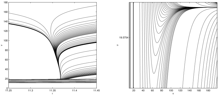
$(a)$ $(b)$

FIG. 1.: The evaporation of a Schwarzschild black hole. (a) The radius as a function of $v$ along a sequence of an outgoing $u=const$ null rays. The rays are emitted from the bottom left corner at different $u=const$ moments. In the late $u$ times the rays begin to curve towards the $r=0$ singularity. There are, however, rays which curve back toward the singularity, but then managed to escape to infinity, indicating the decrease of mass – the evaporation. (b) The contour lines of the radius in $uv$-plane, in a vicinity of the event horizon (defined as a last ray to escape the $r=0$ singularity). The radius decreases from the bottom to the top. The apparent horizon occurs in the locus of $r_{v}=0$ and its radius decreases – a clear evidence for evaporation.

Figure 1(a) depicts the radius as a function of the outgoing null coordinate $v$ along a sequence of an outgoing $u=const$ null rays. The evaporation is mandatory from this picture. Rays which initially incline towards the central $r=0$ singularity manage at some later moment (at the apparent horizon, where $r_{v}=0$) to escape to infinity. The evaporation is indicated by the decreasing radius of the apparent horizon. Figure 1(b) displays the radius contour lines in the $uv$-plane. The apparent horizon is indicated by vanishing of the $r_{v}$ derivative. Again, the decrease of this radius is clear. In passing, we note that our null coordinates are not very convenient to resolve the evaporation of a neutral black holes. The evaporation is contained within a tiny $u$ lapse. The convenient choice is the null coordinates defined at infinity [9]. In these coordinates the evaporation takes an infinite (retarded) time. We did not used these coordinates since our target is the entire spacetime of an evaporating charged black hole. Therefore, we need a set of coordinates which are regular on the outer horizon in order to push the integration inside the black hole. Our original coordinates, being Kruskal-like, supply this set. We find out that our results are in agreement with the previously established ones [9, 10] and turn to the main concern of this work – the evaporation of charged black holes.

We have set the rest of the free parameters as: $v_{1}=5,v_{2}=14,v_{2}^{\prime}=v_{3},v_{f}=2000,A=0.35,B=0.43$ and $e=0.151$. The Figures below are obtained with this specific choice of the parameters. Figure 2(a) displays the radius $r(u,v)$ as a function of the advanced time $v$ along a sequence of $u=const$ outgoing null rays. The retarded time $u$ increases from the rightmost ray to the leftmost one. The rays are emitted from the surface of a collapsing matter (at the left bottom corner). The first rays, which escapes to infinity, are unaffected by the matter indicating the asymptotic flatness of the spacetime. As the collapse proceeds the rays begin to curve back towards the origin. Without evaporation there would be a ray which does not escape to infinity, but stays at a constant radius, this ray indicates the event horizon. The rays emitted after that would asymptotically ($v\rightarrow\infty$) become vertical indicating the formation of the Cauchy horizon (CH) [12, 13]. Finally, the rays emitted in late retarded time would inevitably fall into the strong central singularity. In Figure 3 we depict the ${rv}$-diagram obtained in the classical case, a case without evaporation.

Inclusion of the evaporation changes this picture, specifically the inner and the outer horizons are not stationary null hypersurfaces. Figure 2(c) depicts the enlarged part of Figure 2(a) – the part where the outgoing rays curve to be swallowed by the formed black hole, but then managed to escape to infinity. The locus of the turn-points of these outgoing rays indicates the outer apparent horizon. Figure 2(b) displays another enlarged part of Figure 2(a)– the part where the outgoing rays tend towards the CH. The incline of these, classically vertical, rays towards the outer horizon (above the thick dashed line, see Figure) can be observed. The turn-points (i.e. vanishing of the $r_{v}$ derivative) of these rays indicate the inner apparent horizon.

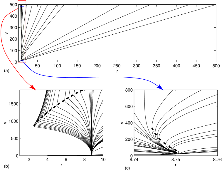
FIG. 2.: The evaporating charged black hole. Figures depict radius $r(u,v)$ as a function of the advanced time $v$ along a sequence of $u=const$ outgoing null rays. The retarded time $u$ grows from the rightmost ray to the leftmost one. (a) The entire spacetime for a charged collapse. (c) The part of (a) in the vicinity of the outer apparent horizon (signaled by vanishing of the $r_{v}$ derivative), which displayed as a thick dashed line. The horizon initially grows, indicating absorption of a matter and formation of a black hole. After that the horizon contracts, indicating the loss of mass by the evaporation. (b) The part of (a) in the vicinity of the inner apparent horizon (again it is signaled by vanishing of the $r_{v}$ derivative), this horizon is displayed as a thick dash-dotted line. Note that the horizons “move” to approach asymptotically ($v\rightarrow\infty$) each other.

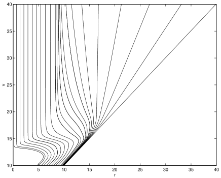
FIG. 3.: The classical collapse. The radius $r(u,v)$ as a function of the advanced time $v$ along a sequence of $u=const$ outgoing null rays. The retarded time $u$ grows from the rightmost ray to the leftmost one. There is an outer apparent horizon located at about $r\approx 16$ (not shown) and the CH indicated by the vertical rays (see further discussion in Ref. [12, 13]).

To gain a further insight into the emerging spacetime we depict in Figure 4 the radius contour lines in $uv$-plane. We show explicitly the inner apparent horizon (a thick dashed line) and the outer apparent horizon (a thick dot-dashed line). The outer horizon initially grows from zero, that corresponds to the formation of a black hole and then it shrinks signaling on the mass-evaporation. The inner horizon (CH) does not remain a contracting null hypersurface, as in a case without evaporation, but instead it expands outwards to meet asymptotically the outer horizon.

The spacetime of the EBH has a very different structure from the non-extremal one, in particular the outer and the inner horizons are located at the same radial coordinate. In the evolutionary context, where the initially non-extremal black hole evolves towards the EBH, the merge of the both horizons will occur in an infinite advanced time (as $v\rightarrow\infty$). The numerical simulation can proceed only to finite values of $v$, and the horizons will only tend to approach each other. We indeed observe this during the simulation. The outer horizon (indicated by tick dotted line in Fig.2(b)) approaches the inner horizon (indicated by tick dashed line in Fig.2(c)). The same picture is seen in Fig. 4. It should be noted that the shrinking of the outer apparent horizon is contained within a small variation of the $u$ coordinates, as in a neutral collapse. That’s because of a Kruskal-like nature of our coordinates.

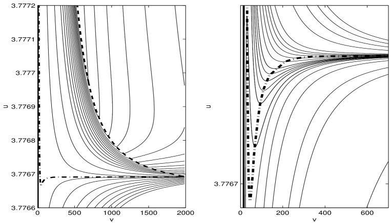
FIG. 4.: Left panel: lines of constant radius in $uv$-plane. The inner and the outer apparent horizons of an evaporating black hole are defined by vanishing of the $r_{v}$ derivative. The inner horizon (shown by thick dashed line) is approaching the outer horizon (the thick dash-dot line) in the asymptotically late advanced time, $v\rightarrow\infty$. Right panel: lines of constant radius in $uv$-plane in a vicinity of the event horizon. The outer apparent horizon is designated by the thick dash-dot line. This horizon contracts from about $v\approx 50$, indicating the mass-evaporation. On the both panels the radius is decreasing from the bottom to the top.

It was interesting to compare the shrinking of the radius of the outer apparent horizon with the radius of this horizon, as it is calculated assuming the external RN metric. In the latter case the radius of the horizon is given by:

$$r_{+}=M+\sqrt{M^{2}-Q^{2}}\ .$$ (11)

Here and below $M\equiv M_{\rm AH}(u,v)$ and $Q\equiv Q_{\rm AH}$ is the mass and the charge of the apparent black hole. In Figure 5 we depict the radius of the outer apparent horizon vs. the advanced time. One can observe that the numerically calculated radius of the horizon (designated by the circles in Figure) and the one obtained by the above formula (solid line) practically coincide. It must not be confusing, despite this remarkable result, the entire spacetime of the dynamically evaporating black hole is very different from the RN one. The radius of the inner horizon, defined in a RN spacetime as $r_{-}=M-\sqrt{M^{2}-Q^{2}}$ does not coincide with the calculated inner horizon. This is because of presence of energy influx which changes the mass-function inside the black hole. This mass-function is different from the external one, $M_{\rm AH}$.

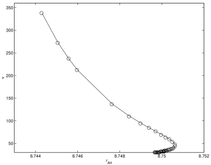
FIG. 5.: The location of the outer apparent horizon of the evaporating black hole as a function of the advanced time $v$.The horizon initially grows indicating the absorption of matter by the black hole. Subsequently (starting from $v\approx 50$) the horizon contracts, signaling on evaporation. The circles represent the numerically obtained radius of the horizon. The solid line represents the location of the horizon, which was calculated assuming RN metric, according to Eqn. (11). The notable similarity of the results shows that a charged black hole is indeed a RN black hole during its evolution, from a point of view of an observer at infinity.

The Hawking-Bekenstein temperature of a RN black hole, as it measured in infinity is defined as:

$$T={\sqrt{M^{2}-Q^{2}}\over{2\pi r_{+}}}\ .$$ (12)

In Figure 6(a) we plot the dependence of the temperature of the dynamical black hole on the advanced time $v$. The temperature is seen to decrease. We note that the obtained black hole is close to a EBH as $1-Q/M\approx 1/400$.

Another quantity of interest is the mass-loss rate. This can be calculated from a negative infalling energy flux $\langle T_{vv}\rangle$, which expected to drive black hole mass-evaporation according to:

$${dM\over dv}={\langle T_{vv}\rangle|}_{AH}\ .$$ (13)

Figure 6(b) depicts the explicitly calculated infalling energy flux $\langle T_{vv}\rangle$ along the outer apparent horizon as a function of an advanced time $v$. The negative influx approaches zero value with the lapse of the advanced time $v$. This corresponds to the stable point in the evolution of the black hole. The black hole tends towards the EBH state, which would be reached at an infinite lapse of $v$.

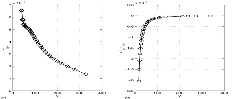
FIG. 6.: (a)The Hawking-Bekenstein temperature $T$ of a black hole as a function of an advanced time $v$ along the outer apparent horizon. The temperature decreases as the black hole evaporates and approaches the EBH state. (b)The negative influx ${\langle T_{vv}\rangle|}_{AH}$ as a function of $v$. The flux tends to the zero value in the late advanced time.

B Evaporation with Discharge

In the next stage of the analysis we relax the assumption of a stable charge, allowing it to be radiated away via the Schwinger pair creation process. We assume that charged particles are not produced in the Hawking process. We examine analytically the fate of a simultaneously evaporating and discharging black hole.

We suppose that the discharge begins only when the electric field of the collapsing matter approaches the critical value, $E_{c}$, and there is no pair creation for the subcritical fields. This is justified since the rate of pair creation for subcritical fields is exponentially suppressed (see e.g.[16]).

Figure 7 is the QM-diagram. The black hole can only form if $Q\leq M$ thus only the region below $M=Q$ is allowed. $M=Q$ is designated by the dashed line in this Figure. The solid line represents black holes for which: $E={Q/r_{+}^{2}}=E_{c}$ along the outer horizon. Below this line the electric field upon the outer horizon is subcritical and charged particles are not produced. Using (11) we find the equation of this trajectory:

$$M(Q,E_{c})={1\over 2}\sqrt{Q\over E_{c}}+{1\over 2}\sqrt{E_{c}\over Q}Q^{2}.$$ (14)

This line intersects the $Q=M$ EBH line at $Q=E_{c}^{-1}$. After the intersection the line continues to the unphysical, $Q>M$, region.

A trajectory of a black hole that evaporates, starting from an initial mass and charge, is represented by a horizontal line in this diagram. If this trajectory intersects the $E=E_{c}$ line it signals the onset of discharge. We depict such a trajectory (dash-dot line in the diagram) that all the three lines intersect at the same point, $Q=E_{c}^{-1}$, the point C in Figure 7. The black holes that evolve along horizontal trajectories lying above the dash-dot line never experience a critical pair-creating field along their horizon. These black holes do not discharge but rather settle down to the stable EBH state. The fate of the black holes that do experience critical field is completely different.

We show below that the following scenario holds. Black holes which evaporate along trajectories, lying below the dash-dot track reach the pair creating field at some moment. Then the black hole evolve along the $E=E_{c}$ line discharging and evaporating simultaneously, decaying to a zero size. If the black hole evaporates exactly on the dash-dot track then it moves towards point C. Here we must recall that a small number of pairs will be produced even for a subcritical field. This small amount of pairs is sufficient to reduce (just a little) the charge of a black hole, pushing it away from the point C towards the decaying regime. This behavior will hold also for a small region above C as long as the pair creation is not suppressed exponentially.

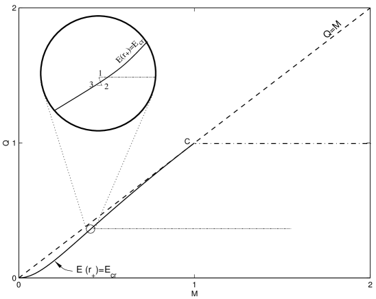
FIG. 7.: A QM-diagram. Black holes can exist only in region below $Q=M$ track, designated here by the dotted line. The solid line in the diagram corresponds to the black holes which experience an extremal pair-creating electric field along their outer horizon. An evaporating black hole is presented in this diagram as a horizontal line. There is the limiting value of charge for an evaporating black hole, such that a black hole having charge above this value will not discharge but rather settle down to an EBH state. We depict a trajectory (dash-dot track) for a limiting black hole.

Let us consider an evaporating black hole, moving along a horizontal line in the region below the dash-dot track. At some moment this black hole will approach the $E(r_{+})=E_{c}\equiv{Q/r_{c}^{2}}$ line. Suppose that the black have evolved slightly into the region above that line. The electric field along its outer horizon is now supercritical and pairs are intensively created. The created pairs reduce the charge of a black hole to the value $Q_{c}$ defined by ${Q_{c}/r_{+}^{2}}=E_{c}$. The pairs being created in the vicinity ($1-{r_{+}\over r_{c}}\ll 1$) of the outer horizon of the black hole are swallowed by it. This forces the increase, $\Delta M$, of the mass of a black hole and therefore increase of the radius of the outer horizon $r_{+}\rightarrow r_{+}^{\prime}>r_{+}$. The electric field along $r_{+}$ is exactly critical and therefore along $r_{+}^{\prime}$ is subcritical. As a result the black hole moves outwards away from the supercritical region. The black hole has evolved $(M,Q)\rightarrow(M^{\prime},Q_{c})$ with $M^{\prime}=M+\Delta M$ during the pair creating stage. In the next stage the black hole evaporates until reaching (and maybe exceeding) again the critical field along its horizon. At the end of this phase the black hole would evolve $(M^{\prime},Q_{c})\rightarrow(M^{\prime\prime},Q_{c})$. If the electric field along the outer horizon is supercritical the above story takes place once again and so on until the full decay. The cycle $(M,Q)\rightarrow(M^{\prime},Q_{c})\rightarrow(M^{\prime\prime},Q_{c})$ is indicated by the cycle 1-2-3 in the zoom-insert in Figure 7. The processes in nature are not discrete as we presented it but rather continuous and both phases take place simultaneously.

The conclusion from the above considerations is clear – the black holes will evolve along the $E(r_{+})=E_{c}$ track after approaching it. Along this track it satisfies

$${dM\over dQ}={1\over 4}\sqrt{1\over E_{c}Q}+{3\over 4}\sqrt{E_{c}Q}\ ,$$ (15)

as obtained by differentiating Eq. (14).

It is also of interest to calculate the mass- and the charge-loss rates of a black hole evolving along the $E(r_{+})=E_{c}$ line. To address this question we implement the idea that if the electric field of a black hole exceeds the critical pair-creating value then the number of created pairs is not simply $N_{0}={Q_{c}-Q\over e}$, but rather enormously amplified. This observation was previously made in [17], tough the calculation we present below differs from that in Ref. [17]. The energy of the created pairs, $\epsilon_{p}$, is extracted from the energy of the electric field of the black hole. If the electric field exceeds only slightly the critical value (that holds for $1-{r_{+}\over r_{c}}\ll 1$ in our circumstance) then the pairs are created nearly at their rest energy with very little kinetic energy. This is in fact the definition of the critical pair-creating field. Therefore, the number of the created pairs can be estimated as $N_{p}\approx{\epsilon_{p}/m}=\Delta M/m$ and $N_{p}\gg N_{0}$ (holding for $e/m\gg 1$). The pairs are created in the region $(r_{+},r_{c})$ with the proper thickness of $\delta r\equiv r_{c}-r_{+}$. The pairs constituting that region are in a state of the quasi-neutral plasma. Only the outermost and the innermost layers of this shell have an uncompensated charge of $Q-Q_{c}$ and the number of pairs in these layers is indeed $N_{0}$ [17].

The rate of the pair creating process at a given radius within the pair-creating region can be approximated as

$$\Gamma={dN\over\sqrt{-g}d^{4}x}={1\over 4\pi}{\left(eE\over\pi\right)}^{2}e^{-{\pi E_{c}\over E}}\ .$$ (16)

From this we can estimate the time needed to create the $N_{p}$ pairs as

$$\Delta\tau_{dis}\approx{N_{p}\over\Gamma V}\ ,$$ (17)

where $V$ is the proper volume of the pair creating region. Using the above results we can estimate the mass increase and the charge loss by the black hole due to discharge.

The charge loss is estimated as $\dot{Q}=e{dN_{0}\over d\tau}\approx{Q-Q_{c}\over\Delta\tau_{dis}}\approx{Q-Q_{c}\over N_{p}}\Gamma V$. The total energy of pairs and therefore the mass increase, $\Delta M$, of the black hole is estimated knowing the initial, $Q/r^{2}$, and the final, $Q_{c}/r^{2}$ electric field configurations

$$\Delta M\approx{Q^{2}-Q_{c}^{2}\over 2r_{+}}\ .$$ (18)

Here we have ignored the energy carried by the $N_{0}$ particles, repulsed to infinity since $N_{p}\gg N_{0}$. Using Eq. (18) to calculate $N_{p}=\Delta M/m$ one obtains, using $\delta r\ll r_{+}$, the charge loss

$$\dot{Q}\approx{2r_{+}\over Q+Q_{c}}m\Gamma V\approx{r_{+}\over Q}m\Gamma V\ .$$ (19)

In the evaporation phase the mass is radiated away by the Hawking process. In order to estimate this rate of mass loss we assume that the black hole radiates as a black body with temperature T, defined by (12), and surface area ${\cal A}=4\pi r_{+}^{2}$. Hence we obtain the approximate mass-evaporation rate:

$${\dot{M}}_{ev}\equiv H\approx\sigma T^{4}\cal A\ ,$$ (20)

where $\sigma$ is the Stefan-Boltzmann constant.

Both processes of evaporation and discharge are simultaneous. The evaporating black hole approaches and exceeds slightly, say by $\delta r$, the critical radius $r_{c}$. The value of $\delta r$, which defines the volume of the pair-creating region according to $V=4\pi r_{+}^{2}\delta r$, will be determined by the requirement that the ratio ${\dot{M}}/{\dot{Q}}$ is given by (15). That is the black hole evolves nearly along the $E(r_{+})=E_{c}$ line. The rate of the mass loss is given by $\dot{M}=\dot{M}_{ev}-\dot{M}_{dis}=H-{\Delta M\over\Delta\tau_{dis}}\approx H-m\Gamma V$. The rate of the charge loss is given by Eq. (19). Therefore, from

$$\left({dM\over dQ}\right)\equiv{\dot{M}\over\dot{Q}}={H-m\Gamma V\over{\left(r_{+}\over Q\right)}m\Gamma V}\ ,$$ (21)

assuming that $\left({dM\over dQ}\right)={\left({dM\over dQ}\right)}_{E(r_{+})=E_{c}}$ one obtains

$$\dot{M}=H\left(1-{1\over{r_{+}\over Q}{\left({dM\over dQ}\right)}_{E(r_{+})=E_{c}}+1}\right)\ .$$ (22)

With the use of Eqs.(14), (15) and (20) this determines the rate of the mass loss in the combined discharge-evaporation process. We have also to perform the necessary consistency check which assures that $\delta r/r_{+}\ll 1$. From Eqs. (21),(22) and (16) with $\Gamma(E)\approx\Gamma(E_{c})$ one finds that $\delta r/r_{+}\ll 1$ if $1/Mm\ll 1$ i.e. if $\lambdabar/r_{+}\ll 1$, where $\lambdabar$ is the Compton wavelength of the created particles. The last inequality holds until the very late stages of the decay when the discharge occurs also via the Hawking process. Hence until the late phases of decay our calculation remains reliable.

Since ${r_{+}\over Q}\left({dM\over dQ}\right)_{E(r_{+})=E_{c}}$ is positive and both ${r_{+}\over Q}>1$ and $\left({dM\over dQ}\right)_{E(r_{+})=E_{c}}>1$, the rate (22) of decay of charged black hole is slower than that of the uncharged evaporating one $\dot{M}<H$ and together $H>\dot{M}>H/2$. Therefore the life-time of the evaporating and discharging black hole is longer than the life-time of an evaporating neutral black hole of the same mass. This is readily understood – what we have after all is the conversion of electrostatic energy of a black hole to the mass, which is radiated away as a Hawking radiation. Since that effective mass exceeds $M$ (approximately by the energy of the electric field), the process of decay lasts more time.

Clearly the decay as we describe it is valid only above the Planck scales, where our (semiclassical) approximation breaks down in favor of full Quantum gravity.

V Summary and Conclusion

We have investigated the formation and evaporation of charged black holes. In the first stage of analysis we assumed stability of the charge, while allowing an evaporation and a decrease of the mass via Hawking radiation. The evaporation was modeled by introducing the expectation value of a 2D stress-energy tensor of a 2D quantized scalar field as a source to the semiclassical Einstein equations. By doing so, we disregard possible contributions which arise from the dimensional reduction procedure [8]. The source which we utilized is (at least) a part of the full 4D stress-energy tensor, and it gives a feeling of the full back-reaction.

We find that the evaporating black hole loses its mass and approaches asymptotically a stable endpoint corresponding to the extremal black hole. Starting from an initially regular matter distribution we have dynamically obtained a non extremal black hole and than, after evaporation, a near extremal one. The outcome of our analysis is the entire dynamical spacetime of such a black hole.

The spacetime structure of a non extremal and an extremal black holes are very different. The most striking feature of the latter is that its inner and outer apparent horizons are located at the same radial coordinate. In the dynamical context we observe that the horizons tend to approach each other in a late advanced time. The actual merge will occur indeed in an infinite (advanced) time, i.e. as $v\rightarrow\infty$. Thisis in agreement with the unattainability formulation of the third law of the black hole thermodynamics. The stability of the final EBH state is manifest from the vanishing of the negative energy influx, $\langle T_{vv}\rangle$, governing the black hole evaporation according to Eq. (13). The Hawking-Bekenstein temperature decreases as the black hole approaches the EBH state.

We have also considered a collapse with evaporation accompanied by a discharge due to instability of the vacuum in strong electric fields. In this case there is a limiting value of charge for a given mass such that black holes with a charge above this value would not discharge but rather evaporate towards a stable EBH state. Black holes with a charge below the limiting charge evaporate and discharge simultaneously, decaying to zero size. It is interesting to note that such black holes are pushed away from the EBH state. The discharge thus prevents from small black holes to become extremal. The life time of an evaporating and discharging black hole is longer then that of an uncharged black hole of the same mass that decays to zero emitting Hawking radiation.

Note added: When this work was completed its brought to our attention that there are related works [18] considering evaporation of 2D RN black holes.

ACKNOWLEDGMENTS: The research was supported by a grant from the Israel Basic Research Foundation.

^∗Electronic address: sorkin@merger.phys.huji.ac.il

^†Electronic address: tsvi@nikki.phys.huji.ac.il

REFERENCES

- [1] W. Israel, Phys.Rev.Lett. 57, 397 (1986).
- [2] T. Jacobson, Phys.Rev. D57, 4890 (1998).
- [3] A. Strominger and S.P. Trivedi, Phys.Rev.D48, 5778 (1993).
- [4] D.A. Lowe and M. O’Loughlin, Phys.Rev. D48, 3735 (1993).
- [5] N.D. Birrell and P.C.W. Davies,Quantum Fields In Curved Space, Cambridge University Press 1982.
- [6] P.C.W. Davies, S.A. Fulling, W.G. Unruh, Phys.Rev. D13, 2720 (1976).
- [7] D. Page, Phys.Rev. D13, 198 (1976).
- [8] For a review see: R. Balbinot and A. Fabbri, Phys.Rev.D59 044031 (1999).
- [9] R. Parentani and T. Piran, Phys. Rev. Lett. 73, 2805 (1994).
- [10] S. Ayal and T. Piran, Phys.Rev. D56, 4768 (1997).
- [11] R.S. Hamadé and J.M. Stewart, Class. Quantum Grav. 13, 497 (1996).
- [12] S. Hod and T. Piran, Phys. Rev. Lett. 81, 1554 (1998); Gen. Rel. Grav. 30, 1555 (1998).
- [13] E. Sorkin and T. Piran, Phys.Rev.D63 084006 (2001).
- [14] L.M. Burko and A. Ori, Phys.Rev. D56, 7820 (1997).
- [15] W.H. Press, S.A. Teukolsky, W.T. Vetterling and B.P. Flannery, Numerical Recipes in Fortran: The Art of Scientific Computing, 2nd ed. Cambridge University Press 1992.
- [16] A.A. Grib, S.G. Mamaev, V.M. Mostepanenko, Quantum Effects in Strong Fields, Atomizdat, Moscow, 2nd ed. 1988 (in Russian).
- [17] G. Preparata, R. Ruffini, S.S. Xue, astro-ph/9810182; R. Ruffini, astro-ph/9811232.
- [18] A.Fabbri, D.J.Navarro, J.Navarro-Salas Phys.Rev.Lett. 85 (2000) 2434 ; and Nucl.Phys. B595 (2001) 381.