CU-TP-1013

Two Black Hole Holography, Lensing and Intensity

Mark G. Jackson

Department of Physics

Columbia University

New York City, NY 10027

We numerically verify the analysis of the “expanding horizon” theory of Susskind in relation to the ’t Hooft holographic conjecture. By using a numerical simulation to work out the holographic image formed by two black holes upon a screen very far away, it is seen that it is impossible for a horizon to hide behind another. We also compute the holographic intensity distribution of such an arrangement.

1 Introduction

In 1988 ’t Hooft made the surprising announcement that the world had one less dimension than previously believed [1]. This was based on the number of degrees of freedom in a given region of space, being found not to depend on the volume, as might be naively expected, but rather on the surface area containing the volume. Furthermore, this conclusion connected with one of the few nontrivial combinations of gravity and quantum field theory, the entropy content of a black hole [2]. ’t Hooft went on to claim that this idea of dimensional reduction, or “holography,” would need to be present in any unifying theory.

At the time of ’t Hooft’s hypothesis string theory was not yet understood at a level that such a claim could be tested in that area (indeed, Maldacena later found precisely this feature [4]). Susskind was able to show that this claim had validity in General Relativity [3]; if it was true that the entropy density of a surface was maximal on that bounding a black hole, then this area must expand when projected onto a screen far away. In this computation we count only the geodesics orthogonal to the screen, since we are not allowed any information which may depend on the screen’s position; a geodesic which is nonperpendicular to the screen will intersect in different locations depending on the screen’s position. This “expanding horizon” theory of Susskind was explicitly verified by Corley and Jacobson [5] for the single black hole case. But another observation of Susskind’s was that the information in a second black hole was not allowed to hide behind the first, with respect to the screen; the geodesics will arrange themselves to project all information to the screen with non-increasing entropy density. Corley and Jacobson quote a magnification factor of the black hole image at large separation, but no examples were given. In this paper we explicitly calculate the geodesics in a two Schwarzschild black hole geometry. Black hole lensing has been carried out previously [6] [7] but to our knowledge not for two black holes, which has the novel feature of an arbitrary number of orbits between them before the photon escapes. Furthermore, the geometry used easily lends itself to a calculation of the holographic intensity pattern formed by a uniformly radiating black hole (the intensity pattern formed keeping only the geodesics perpendicular to the screen). We also perform this calculation.

2 Single Black Hole

2.1 Calculation of Orbits

Beginning with the Schwarzschild black hole metric normalized to $r=1$ at the horizon,

$$ds^{2}=\left(1-\frac{1}{r}\right)dt^{2}-\frac{dr^{2}}{1-1/r}-r^{2}d\theta^{2}-r^{2}\sin^{2}\theta d\phi^{2},$$ (2.1)

the null geodesic equation can be put into the form $(s\equiv 1/r)$

$$d\phi=\frac{ds}{\sqrt{b^{-2}-s^{2}(1-s)}}$$ (2.2)

where $b$ is the impact parameter and $\phi$ is the azimuthal angle in the plane of our choosing. It is most useful to do the integration “backward,” in the sense that we begin at the screen and track the geodesic until it has hit the horizon or has deflected away from the black hole. We will first work out the case where the geodesic hits the horizon, then calculate the case where it deflects off one black hole to hit another.

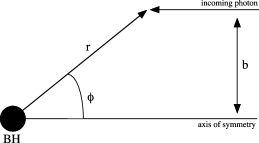
Figure 1: A photon approaching a single Schwarzschild black hole from the screen infinitely far away.

Integrating from $r=\infty$ to $r=1$ means $s$ goes from 0 to 1. Using the photon’s incoming line of flight to define $\phi=0$, we get

$$\phi(b)=\int^{1}_{0}\frac{ds}{\sqrt{b^{-2}-s^{2}(1-s)}}.$$ (2.3)

The denominator vanishes at $b_{c}=\frac{3\sqrt{3}}{2}$, indicating that is the largest value of $b$ for which we can establish a map between the screen and the black hole. Before that, though, the integral (or angle of the photon upon absorption) goes from 0 to infinity, implying that there exists some $b$ for which the photon will orbit around the black hole indefinitely before finally being absorbed. Corley and Jacobson [5] define a “covering” to be one complete image of the horizon upon the screen; the first covering is due to emission from the black hole between $\phi=0$ and $\phi=\pi/2$, the second covering from $\phi=\pi/2$ to $\phi=\pi$, as shown in figure 2.

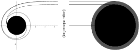
Figure 2: Null geodesics showing boundaries of the first few coverings (left) and the corresponding screen image (right).

We obtained the result found in [5] that the maximal impact parameter for the first covering is $b\approx 2.23$; this represents an area of 15.60, larger than the horizon area $4\pi\approx 12.57$. Successive coverings are smaller than this on the screen.

2.2 Intensity

We now compute not just the location of the coverings on the screen, but the intensity pattern a “holographic viewer” would observe, i.e. a viewer only capable of observing geodesics perpendicular to the screen. This is based upon a black hole radiating uniformly on its surface, then calculating the density of geodesics orthogonal to the screen. The first step is to calculate the angle $\psi$ at which the geodesic hits the black hole,

$$\left.\tan\psi\right|_{\it surface}=\left.\frac{r}{dr/d\phi}\right|_{s=1}.$$ (2.4)

For us,

$$\frac{dr}{d\phi} = \frac{dr}{ds}\frac{ds}{d\phi},$$ (2.5)

$$= \frac{1}{s^{2}}\sqrt{b^{-2}-s^{2}(1-s)}.$$

Thus we obtain $\left.\tan\psi\right|_{s=1}=b$.

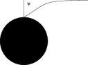
Figure 3: A geodesic will hit the black hole at an angle.

The intensity of a point on the screen will be the ratio of geodesic phase space between the screen and the corresponding point on the black hole, so we must allow our photon to have small variations from the geodesic path. We begin with the standard case of a ray leaving $\psi(b)$ from the normal (see Figure 3) and leaving the BH in the plane at angle $\phi(b)$; let us now think of $\psi$ as the independent variable and refer to $\phi(b)$ as $\phi(\psi)$. The geodesic impacts the screen at $(x,y,z)=(0,b(\psi),Z)=(0,\tan\psi,Z)$. Now rotate the BH clockwise in the z-y plane by angle $\phi(\psi)$, making the ray hit the screen at

0cosϕ(ψ)−sinϕ(ψ)0sinϕ(ψ)cosϕ(ψ))​( tanψZ)𝑥𝑦𝑧fragments 0fragmentsϕ(ψ)fragmentsϕ(ψ)0fragmentsϕ(ψ)fragmentsϕ(ψ) fragmentsψ𝑍\left(\begin{tabular}[]{c}$x$\\ $y$\\ $z$\end{tabular}\right)=\left(\begin{tabular}[]{ccc}$1$&$0$&$0$\\ $0$&$\cos\phi(\psi)$&$-\sin\phi(\psi)$\\ $0$&$\sin\phi(\psi)$&$\cos\phi(\psi)$\end{tabular}\right)\left(\begin{tabular}[]{c}$0$\\ $\tan\psi$\\ $Z$\end{tabular}\right)

10001000 (2.6)

so it appears as though the ray were leaving from the BH on the $z$ axis; we will call this transformation $J_{1}$. Now rotate around the z axis so that the ray is leaving at an angle $\theta_{2}$ from the y-z plane,

$$J_{2}=\left(\begin{tabular}[]{ccc}$\cos\theta_{2}$&$-\sin\theta_{2}$&$0$\\ $\sin\theta_{2}$&$\cos\theta_{2}$&$0$\\ $0$&$0$&$1$\end{tabular}\right).$$ (2.7)

Rotate back by arbitrary $\phi$ in the y-z plane

0cosϕsinϕ0−sinϕcosϕ).subscript𝐽3fragments 0fragmentsϕfragmentsϕ0fragmentsϕfragmentsϕJ_{3}=\left(\begin{tabular}[]{ccc}$1$&$0$&$0$\\ $0$&$\cos\phi$&$\sin\phi$\\ $0$&$-\sin\phi$&$\cos\phi$\end{tabular}\right).

100100 (2.8)

Finally rotate around the z-axis again by arbitrary angle $\theta$,

$$J_{4}=\left(\begin{tabular}[]{ccc}$\cos\theta$&$-\sin\theta$&$0$\\ $\sin\theta$&$\cos\theta$&$0$\\ $0$&$0$&$1$\end{tabular}\right).$$ (2.9)

Then the final location of the photon is

tanψZ).𝑥𝑦𝑧subscript𝐽4subscript𝐽3subscript𝐽2subscript𝐽1 fragmentsψ𝑍\left(\begin{tabular}[]{c}$x$\\ $y$\\ $z$\end{tabular}\right)=J_{4}J_{3}J_{2}J_{1}\left(\begin{tabular}[]{c}$0$\\ $\tan\psi$\\ $Z$\end{tabular}\right).

$$\left(\begin{array}{c}x\\ y\\ z\end{array}\right)=J_4{J}_3{J}_2{J}_1(\begin{array}{c}\end{array}$$00 (2.10)

Thus we can define our new impact parameter $b^{\prime}\equiv\sqrt{x^{2}+y^{2}}$, but clearly upon $\theta=\theta_{2}=0,\phi=\phi(\psi)=\phi(b),\psi=\psi(b)$ where $b$ is some parameter of our choosing, we recover $b^{\prime}=b$. We also take the $Z\rightarrow\infty$ limit since that is where the screen is. To compare the areas of the BH and screen, we compute

$$\left.\frac{d(\cos\phi)\ d\theta}{b^{\prime}\ db^{\prime}\ d\theta}\right|_{\theta=\varphi=0,\phi=\phi(b),\psi=\psi(b^{\prime}),b^{\prime}=b,Z\rightarrow\infty} = \left.\frac{\sin\phi}{b^{\prime}}\left(\frac{db^{\prime}}{d\phi}\right)^{-1}\right|_{...}$$ (2.11)

$$= \left.\frac{\sin\phi}{b^{\prime}}\left(\frac{1}{\sqrt{x^{2}+y^{2}}}\left(x\frac{dx}{d\phi}+y\frac{dy}{d\phi}\right)\right)^{-1}\right|_{...}$$

$$= \left.\frac{\sin\phi(b)}{b}\left(Z+O(1/Z^{2})\right)^{-1}\right|_{z\rightarrow\infty}$$

$$= \frac{1}{Z}\frac{\sin\phi(b)}{b}.$$

We now examine at how the photon’s tangent vector at the screen changes under these transformations. We know it begins hitting the screen perpendicular, and then will undergo the same transformations as the position vector:

$$\left(\begin{tabular}[]{c}$x$\\ $y$\\ $z$\end{tabular}\right)=J_{4}J_{3}J_{2}J_{1}\left(\begin{tabular}[]{c}$0$\\ $0$\\ $1$\end{tabular}\right).$$ (2.12)

Now define the angle that it hits the screen at as $\sin\psi^{\prime}\equiv\sqrt{x^{2}+y^{2}}$ and the angle out of the y-z plane as $\tan\varphi\equiv x/y$. Then we have the following tangent vector phase space comparison between the ray leaving the black hole and that hitting the screen:

$$\left.\frac{d(\cos\psi)\ d\theta_{2}}{d(\cos\psi^{\prime})\ d\varphi}\right|_{...} = \left.\frac{\sin\psi}{\sin\psi^{\prime}}\left(\frac{d\psi^{\prime}}{d\psi}\right)^{-1}\left(\frac{d\varphi}{d\theta_{2}}\right)^{-1}\right|_{...},$$ (2.13)

$$= \frac{\sin\psi}{\sin\psi^{\prime}}\left(\frac{1}{\sqrt{1-x^{2}-y^{2}}}\frac{1}{\sqrt{x^{2}+y^{2}}}\left(x\frac{dx}{d\psi}+y\frac{dy}{d\psi}\right)\right)^{-1},$$

$$\times \left(\frac{1}{1+(x/y)^{2}}\left(\frac{1}{y}\frac{dx}{d\theta_{2}}-\frac{x}{y^{2}}\frac{dy}{d\theta_{2}}\right)\right)^{-1},$$

$$= \frac{b}{\sqrt{1+b^{2}}\sin\phi(b)\frac{d\phi(b)}{d\psi}},$$

$$= \frac{b}{\sqrt{1+b^{2}}\sin\phi(b)\frac{d\phi(b)}{db}\frac{db}{d\psi}},$$

$$= \frac{b}{(1+b^{2})^{3/2}\sin\phi(b)\frac{d\phi(b)}{db}}.$$

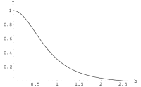
Figure 4: Normalized intensity as a function of impact parameter in a single black hole.

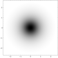
Figure 5: The intensity pattern formed on the screen due to a single black hole.

Combining the phase-space ratios we get the intensity:

$$I(b) = \frac{\textrm{total phase space of rays leaving BH}}{\textrm{total phase space of rays hitting screen}},$$ (2.14)

$$= \frac{d(\cos\phi)\ d\theta\ d(\cos\psi)\ d\theta_{2}}{b^{\prime}\ db^{\prime}\ d\theta\ d(\cos\psi^{\prime})\ d\varphi},$$

$$= \frac{1}{Z}\frac{1}{(1+b^{2})^{3/2}\frac{d\phi(b)}{db}}.$$

The result is shown in Figures 4 and 5. In computing the image we have factored out the $1/Z$ since this represents the obvious dependence on distance and we only care about the intensity normalized at some specific distance.

3 Two Black Holes

3.1 Calculation of Orbits

We now use the techniques developed in the previous section to construct the metric for two black holes; this metric is valid for large separation between the black holes. The axes are chosen so the screen lies in the $x-y$ plane, and the origin is at the position of the first black hole (the one nearer the screen) with the screen is a very large distance down the positive $z$ axis. The second black hole is taken to lie at the point

$$BH_{2}=(\rho\cos\mu,\rho\sin\mu,-D).$$ (3.1)

We construct the scattering process in reverse by considering photons emitted in the normal $(-{\hat{\bf z}})$ direction from the screen, track their geodesics, and pick out those which are absorbed by one of the two black holes. Since varying $\mu$ above rotates the picture about the $z$ axis we consider only photons emitted from points on the screen with $y=0$. So the trajectory describing the scattering off the first black hole lies entirely in the $x-z$ plane.

Figure 6: Obtaining the impact parameter for the second black hole.

The photon is emitted at a distance $b_{1}$ from the $z$ axis. It is deflected with angle $\phi(b)$ by the first black hole. The point $P$ at which the asymptotes meet is

$$P=(r\sin\phi,0,r\cos\phi)$$ (3.2)

where

$$r=\frac{b}{\sin\phi}$$ (3.3)

as evident from the triangle indicated. The direction of the deflected photon (the lower asymptote in the figure) is given by the unit vector

$${\bf v}=(\sin 2\phi,0,\cos 2\phi).$$ (3.4)

Our task is now simply to compute the distance $b_{2}$ of the line with these direction cosines passing through the point $P$ from the point $BH_{2}$. The photon will be absorbed by the second black hole if $b_{2}<b_{c}$.

Drawing the line connecting $P$ and $BH_{2}$, the total length is $L$ and there is an angle $\epsilon$ with ${\bf v}$, making the answer

$$b_{2}=L\sin\epsilon.$$ (3.5)

The vector ${\bf L}$ joining them is

$${\bf L}=BH_{2}-P=(\rho\cos\mu-r\sin\phi,\rho\sin\mu,-D-r\cos\phi)$$ (3.6)

so its length satisfies

$$L^{2}=D^{2}+\rho^{2}+r^{2}-2\rho r\cos\mu\sin\phi+2Dr\cos\phi.$$ (3.7)

To determine $\epsilon$ we use

$$\cos\epsilon=\frac{{\bf L}\cdot{\bf v}}{L}.$$ (3.8)

The inner product is also simple to compute:

$$L\cos\epsilon = {\bf L}\cdot{\bf v}=(\rho\cos\mu-r\sin\phi)\sin 2\phi-(D+r\cos\phi)\cos 2\phi$$ (3.9)

$$= \rho\cos\mu\sin 2\phi-D\cos 2\phi-r(\sin\phi\sin 2\phi+\cos\phi\cos 2\phi)$$

$$= \rho\cos\mu\sin 2\phi-D\cos 2\phi-r\cos\phi.$$

From these we compute simply

$$b_{2}=L\sin\epsilon=\sqrt{L^{2}-(L\cos\epsilon)^{2}}.$$ (3.10)

This impact parameter is then fed into our previous calculations for a single black hole, with appropriate distance normalization due to the mass of the second black hole; remember in our units 1 = 1 horizon unit, and all calculations in this geometry were done based on the horizon of the first black hole. It is immediately obvious that this procedure can be generalized to any number of black holes and “back-and-forth” orbits between them. To get a concrete visualization of this process, we show in Figure 7 the case with $D=10$, $0\leq\rho\leq 20$. In Figure 8 we compute the area of the first covering on the second black hole for $D=10,0\leq\rho\leq 25$. For this we included only the first-covering area to the left of the first black hole, as there is a redundency on the right side and we are only interested in how much area it takes to represent the whole horizon once. The hiding theorem is clearly verified, the horizon expanding even more when it forms a ring.

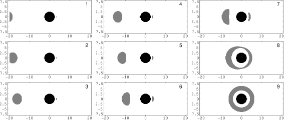
Figure 7: Attempted horizon hiding for $D=10,$ $0\leq\rho\leq 20$. Gray represents the geodesic hitting the second black hole, black indicates hitting the first.

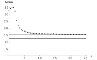
Figure 8: The area of the first covering when attempting to hide. The lower bar indicates the horizon area $=4\pi$, which we need to be above. The upper bar indicates the area of the first covering for a single black hole, which the second black hole must approach at large separation.

3.2 Intensity

Thinking about phase space as before, we see that for two black holes the situation is very similar except we now remember the rays leave the “real” screen, deflect off BH1 to form a “virtual screen,” then hit BH2. Thus

$$I = \frac{\textrm{phase space of rays leaving BH 2 }}{\textrm{phase space of rays hitting real screen}},$$ (3.11)

$$= \frac{\textrm{PS of rays leaving BH 2}}{\textrm{PS of rays hitting virtual screen}}\frac{\textrm{PS of rays hitting virtual screen}}{\textrm{PS of rays hitting real screen}},$$

$$= \frac{1}{(1+b_{2}^{2})^{3/2}\frac{d\phi(b_{2})}{db_{2}}}\frac{\textrm{differential area of virtual screen}}{\textrm{differential area of real screen}}.$$

where the first part is from our previous single BH analysis, and the second is just comparing the differential area containing the ray on the virtual screen versus the real screen. Note that we have omitted the phase space on the screens due to the tangent vector in this step, but this is just unity because both screens by definition only take only perpendicular rays and so have the same tangent phase space. The ratios of differential areas are then

$$\frac{b_{2}\ db_{2}\ d\kappa}{b_{1}\ db_{1}\ d\theta}$$ (3.12)

where $\kappa$ is shown in Fig. 6 and $\theta$ is the usual coordinate around the z axis. We evaluate this by switching to cartesian coordinates $(b_{1},y)$ for BH2:

$$b_{2}\ db_{2}\ d\kappa\rightarrow db_{1}\ dy$$ (3.13)

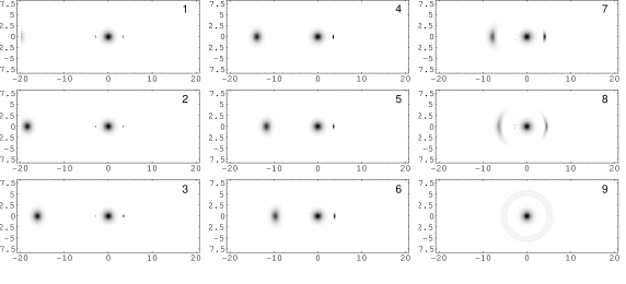
Figure 9: As a black hole hides behind another, the image becomes very faint.

Now see that this yields immediate cancellation with the $b_{1}$. As for $dy$, we see that this point being lifted out of the plane is a distance $b_{min}$ from the z-axis, thus $dy=b_{min}d\theta$. The $d\theta$’s cancel, leaving only $b_{min}/b_{1}$. With

$$b_{min}=b_{1}-L\cos\epsilon\sin(2\phi-\pi)$$ (3.14)

and the expression previously obtained for $L\cos\epsilon$ we get

$$\frac{b_{min}}{b_{1}}=1+\frac{L\cos\epsilon\sin 2\phi}{b_{1}}.$$ (3.15)

So the total intensity is just

$$I=\frac{1}{(1+b_{2}^{2})^{3/2}\frac{d\phi(b_{2})}{db_{2}}}\left(1+\frac{L\cos\epsilon\sin 2\phi(b_{1})}{b_{1}}\right).$$ (3.16)

We now repeat the previous lensing calculation, but including this intensity profile. The result is shown in Figure 9.

4 Conclusion

We have verified Susskind’s hypothesis that the entropy is maximal on the surface of a black hole. We did this for the two black hole case and found that no entropy-information is lost when one black hole attempts to hide behind the other. The holographic intensity of such a configuration was also calculated.

5 Acknowledgements

The author thanks B. Paczynski, H. Peiris, E. Weinberg, and especially R. Plesser for helpful comments.

References

- [1] G. ’t Hooft, “On the Quantization of Space and Time,” in Quantum Gravity: proceedings, ed. M.A. Markov, V.A. Berezin, V.P. Frolov (World Scientific, 1988).
- [2] J. D. Bekenstein, Phys. Rev. D 9 (1974) 3292.
- [3] L. Susskind, J. Math. Phys. 36 (1995) 6377, hep-th/9409089.
- [4] J. Maldacena, Adv. Theor. Math. Phys. 2 (1998) 231, hep-th/9711200.
- [5] S. Corley, T. Jacobson, Phys. Rev. D 53 (1996) 6720-6724, gr-qc/9602043.
- [6] V. Bozza, “Strong field limit of black hole gravitational lensing,” gr-qc/0102068.
- [7] K. S. Virbhadra, “Schwarzschild black hole lensing,” Phys. Rev. D 62 (2000) 084003, astro-ph/9904193