Space missions to detect the cosmic gravitational-wave background

Abstract

It is thought that a stochastic background of gravitational waves was produced during the formation of the universe. A great deal could be learned by measuring this Cosmic Gravitational-wave Background (CGB), but detecting the CGB presents a significant technological challenge. The signal strength is expected to be extremely weak, and there will be competition from unresolved astrophysical foregrounds such as white dwarf binaries. Our goal is to identify the most promising approach to detect the CGB. We study the sensitivities that can be reached using both individual, and cross-correlated pairs of space based interferometers. Our main result is a general, coordinate free formalism for calculating the detector response that applies to arbitrary detector configurations. We use this general formalism to identify some promising designs for a GrAvitational Background Interferometer (GABI) mission. Our conclusion is that detecting the CGB is not out of reach.

1 Introduction

Before embarking on a quest to discover the Cosmic Gravitational-wave Background (CGB), it is worth reflecting on how much has been learned from its electromagnetic analog, the Cosmic Microwave Background (CMB). The recent Boomerang[1] and Maxima[2] experiments have furnished detailed pictures of the universe some 300,000 years after the Big Bang. These measurements of the CMB anisotropies have been used to infer that the visible universe is, to a good approximation, spatially flat. The earlier COBE-DMR[3] measurements of the CMB anisotropy fixed the scale for the density perturbations that formed the large scale structure we see today, and showed that the density perturbations have an almost scale free spectrum. With all this excitement over the anisotropy measurements it is easy to forget how much the CMB taught us before the anisotropies were detected. The initial observation that the CMB is highly isotropic is one of the major observational triumphs of the Big Bang theory. Equally important was the discovery by COBE-FIRAS[4] that the CMB has an exquisite black body spectrum with a temperature of 2.728 Kelvin.

The lesson that we take from the CMB is that while it would be wonderful to have a COBE style map of the early universe in gravitational waves, a great deal can be learned by detecting the isotropic component. The main focus of this work is on the fixing the amplitude of the CGB at some frequency. Some attention will also be given to the prospects of measuring the the energy spectrum. Detecting anisotropies in the CGB is a considerably harder problem that we address elsewhere[5].

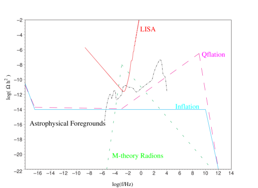
Figure 1: Possible sources of a stochastic gravitational wave background plotted against the sensitivity curve for the LISA mission.

There are two major obstacles that stand in the way of detecting the CGB. The first is the extreme weakness of the signal, and the second is the competing stochastic background produced by astrophysical sources. Figure 1 shows various predictions for the CGB energy spectra in several early universe scenarios including standard inflation, a particular M-theory model[6] and quintessence based inflation[7]. Also shown is the sensitivity curve for the proposed Laser Interferometer Space Antenna (LISA)[8], and a compilation of possible extragalactic astrophysical foregrounds taken from the work of Schneider et al.[9]. The spectrum is expressed in terms of $\Omega_{\rm gw}(f)$, the energy density in gravitational waves (in units of the critical density) per logarithmic frequency interval, multiplied by $h_{0}^{2}$, where $h_{0}$ is the Hubble constant in units of 100 km s^-1 Mpc^-1. The predictions for the CGB power spectra are fairly optimistic, and some of them come close to saturating existing indirect bounds on $\Omega_{\rm gw}(f)$ – see the review by Maggiore for details[10].

With the exception of the M-theory motivated model, we see that the major obstacle to detecting the CGB is not the sensitivity of our detectors, but competition from astrophysical foregrounds. The astrophysical foregrounds are produced by the combination of a great number of weak sources that add together to form a significant stochastic signal. Based on current estimates, it is thought that the contribution from astrophysical sources falls off fairly rapidly below 1 $\mu$Hz. For that reason, we will focus our attention on detecting the CGB in the sub-micro Hertz regime. To put this number into perspective, an interferometer built using LISA technology would need spacecraft separated by one-tenth of a light year to reach a peak sensitivity at 1 $\mu$Hz! A more practical approach is to use two smaller interferometers that lack the intrinsic sensitivity to detect the CGB on their own, but together are able to reach the necessary sensitivity. The idea is to cross correlate the outputs from the two interferometers and integrate over some long observation time $T$. Since the noise in the two interferometers is uncorrelated while the signal is correlated, the signal to noise ratio will steadily improve as the observation time is increased.

In principle, it is possible to detect an arbitrarily weak signal by observing for an arbitrarily long time. In practice, the prospects are not so rosy as the sensitivity of the detector pair only improves on the sensitivity of a single detector as $(T\Delta f)^{1/2}$, where $\Delta f$ is the frequency bandpass. The frequency bandpass is typically taken to equal the central observing frequency. Suppose we try and look for the CGB at a frequency of $f\approx\Delta f=10^{3}$ Hz using the two LIGO detectors. Over an observation time of $T=1$ year, the sensitivity is improved by a factor of $\sim 2\times 10^{5}$ by cross correlating the Washington and Louisiana detectors. For a pair of LISA detectors with a bandpass of $\Delta f\approx 10^{-2}$ Hz, cross correlating for a year would result in a 500 fold improvement in sensitivity. However, for detectors operating in the $\mu$Hz range, cross correlating two detectors for one year only improves on the sensitivity of a single detector by a factor of $\sim 6$. So why use two interferometers when one will do? The reason is simple: with a single interferometer it is not possible to tell the difference between the CGB and instrument noise since both are, to a good approximation, stationary Gaussian random processes. Moreover, it is impossible to shield a detector from gravitational waves in order to establish the noise floor. With two or more independent interferometers the cross correlated signal can be used to seperate the stochastic bacground from instrument noise. The LISA system has three arms, and the signal from these arms can be used to form three different Michelson interferometers. However, these interferometers share spacecraft, and thus common sources of noise, so nothing is gained by cross correlating the outputs. However, Tinto et al.[11] have recently suggested another way of combining the signals, known as a Sagnac system, that creates an interferometer that is fairly insensitive to gravitational waves. Since the response of this “bad” interferometer is noise dominated, its output can be used to estimate the noise floor for the standard interferometer configuration. Thus, a single LISA type observatory might be able to discriminate between the CGB and instrument noise.

We will show that cross correlating two LISA interferometers results in a signal to noise ratio of

$${\rm SNR}=1.4\left(\frac{T}{{\rm year}}\right)^{1/2}\left(\frac{\Omega_{{\rm gw}}h_{0}^{2}}{10^{-14}}\right)$$ (1)

for a scale invariant stochastic gravitational wave background. This represents a five hundred fold improvement over the sensitivity of a single LISA interferometer. If it were not for the astrophysical foregrounds that are thought to dominate the CGB signal in the LISA band, a pair of LISA detectors would stand a good chance of detecting the CGB. In an effort to avoid being swamped by astrophysical sources, we focus our efforts on detecting the CGB below 1 $\mu$Hz. We show that a pair of interferometers can reach a signal to noise of

$${\rm SNR}=3.1\left(\frac{T}{{\rm year}}\right)^{1/2}\left(\frac{\Omega_{\rm gw}h_{0}^{2}}{10^{-14}}\right)\left(\frac{L}{\sqrt{3}\,{\rm AU}}\right)^{2}\left(\frac{3\times 10^{-16}{\rm m}{\rm s}^{-2}}{\delta a}\right)^{2}\left(\frac{f}{\mu{\rm Hz}}\right)^{3/2}$$ (2)

for a scale invariant CGB spectrum. The above result is scaled against a possible LISA follow-on mission (LISA II) that calls for two identical interferometers, comprising six equally spaced spacecraft that form two equilateral triangles overlayed in a star pattern. The constellations follow circular orbits about the Sun in a common plane at a radius of 1 AU, so that each interferometer arm is $L=\sqrt{3}$ AU in length. The acceleration noise, $\delta a$, is scaled against a value that improves on the LISA specifications by one order of magnitude. The LISA II design could detect a stochastic background at 99% confidence with one year of observations if $\Omega_{\rm gw}h_{0}^{2}=10^{-14}$. Ideally we would like to reach a sensitivity of at least $\Omega_{\rm gw}h_{0}^{2}\sim 10^{-20}$ in order to detect inflationary spectra with a mild negative tilt. It is difficult to achieve this with spacecraft orbiting at 1 AU as thermal fluctuations due to solar heating of the spacecraft make it hard to reduce the acceleration noise below $\delta a\simeq 10^{-16}\,{\rm m}{\rm s}^{-2}$. The best strategy is to increase the size of the orbit, $R$, as this increases the size of the interferometer, $L=\sqrt{3}R$, and decreases the thermal noise by $R^{-2}$.

2 Outline

We begin by deriving the response of a pair of cross correlated space-based laser interferometers to a stochastic background of gravitational waves. Similar calculations have been done for ground based detectors[12, 13, 14, 15, 16], but these omit the high frequency transfer functions that play an important role in space based systems. Our calculations closely follow those of Allen and Romano[16], and reduce to theirs in the low frequency limit. Many of the calculational details that we omit for brevity can be found in their paper. Having established the general formalism for cross correlating space based interferometers we use our results to identify some promising configurations for a GrAvitational Background Interferometer (GABI) mission to detect the CGB.

3 Detector Response

We attack the problem of cross correlating two space based interferometers in stages. We begin by reviewing how the Doppler tracking of a pair of spacecraft can be used to detect gravitational waves. Using this result we derive the response of a two arm Michelson interferometer and express the result in a convenient coordinate-free form. The response of a single interferometer is then used to find the sensitivity that can be achieved by cross correlating two space based interferometers.

3.1 Single arm Doppler tracking

Following the treatment of Hellings[17], we consider two free spacecraft, one at the origin of a coordinate system and the other a distance $L$ away at an angle $\theta$ from the $z$ axis. Both spacecraft are at rest in this coordinate system. The spacecraft at the origin sends out a series of photons, while a weak plane gravitational wave is passing through space in the $+z$ direction. To leading order, the spacetime metric in the transverse-traceless gauge is:

$$\quad ds^{2}=-c^{2}dt^{2}+dz^{2}+(1+h\cos 2\psi)dx^{2}+(1-h\cos 2\psi)dy^{2}-h\sin 2\psi dxdy\,,$$ (3)

where $h(t-z/c)$ is the wave amplitude and $\psi$ is the angle between the principal polarization vector and the $x$ axis. If we choose our coordinates such that the second spacecraft is in the $x-z$ plane, the path of the photons can be parameterized by

$$x=\rho\sin\theta\quad\quad z=\rho\cos\theta\,.$$ (4)

The photon path in the perturbed spacetime is given by $ds^{2}=0$, or

$$c\,dt\simeq\pm(1+\frac{1}{2}h\cos 2\psi\sin^{2}\theta)\,d\rho\,.$$ (5)

The round trip journey from spacecraft 1 to spacecraft 2 and back again is given by

$$\quad\ell(t_{2}-t_{0})=\int_{t_{0}}^{t_{2}}c\,dt = 2L+\frac{1}{2}\cos 2\psi\sin^{2}\theta\left(\int_{0}^{L}h[t_{0}+\frac{\rho}{c}(1-\cos\theta)]d\rho\right.$$ (6)

$$\left.\hskip 72.26999pt+\int_{0}^{L}h[t_{1}+\frac{L}{c}-\frac{\rho}{c}(1+\cos\theta)]d\rho\right)\,.$$

Here $t_{0}$ is the time of emission, $t_{1}$ is the time of reception at spacecraft 2 and $t_{2}$ is the time of reception back at the first spacecraft. Using $h(q)=h_{0}\exp(i\omega q)$, the varying portion of the round-trip distance is

$$\delta\ell(t_{2})=L\,h(t_{2})\cos 2\psi\sin^{2}\theta\frac{1}{2} \left({\rm sinc}\left(\frac{f}{2f_{*}}(1-\cos\theta)\right)\exp\left(-i\frac{f}{2f_{*}}(3+\cos\theta)\right)\right.$$ (7)

$$\left.+{\rm sinc}\left(\frac{f}{2f_{*}}(1+\cos\theta)\right)\exp\left(-i\frac{f}{2f_{*}}(1+\cos\theta)\right)\right)\,,$$

where $f=\omega/(2\pi)$ is the frequency of the gravitational wave and $f_{*}=c/(2\pi L)$ is the transfer frequency. To zeroth order in $h$, the optical path length is $\ell=2L$. The general, coordinate independent version of this expression is given by

$$\frac{\delta\ell}{\ell}=\frac{1}{2}({\bf u}\otimes{\bf u}):{\bf h}(\widehat{\Omega})\,{\cal T}({\bf u}\cdot\widehat{\Omega},f)\,,$$ (8)

where $\bf{u}$ is a unit vector pointing from the first to the second spacecraft and $\widehat{\Omega}$ is a unit vector in the direction the gravitational wave is propagating. The colon denotes the double contraction ${\bf a}:{\bf b}=a_{ij}b^{ij}$. The transfer function ${\cal T}$ is given by

$${\cal T}({\bf u}\cdot\widehat{\Omega},f) = \frac{1}{2}\left[{\rm sinc}\left(\frac{f}{2f_{*}}(1-{\bf u}\cdot\widehat{\Omega})\right)\exp\left(-i\frac{f}{2f_{*}}(3+{\bf u}\cdot\widehat{\Omega})\right)\right.$$ (9)

$$+ \left.{\rm sinc}\left(\frac{f}{2f_{*}}(1+{\bf u}\cdot\widehat{\Omega})\right)\exp\left(-i\frac{f}{2f_{*}}(1+{\bf u}\cdot\widehat{\Omega})\right)\right]\,.$$

This expression for ${\cal T}$ agrees with the one derived by Schilling[18]. The gravitational wave is described by the tensor

$${\bf h}(t,{\bf x})=h^{+}(\omega t-\omega\widehat{\Omega}\cdot{\bf x}){\bf\epsilon}^{+}(\widehat{\Omega},\psi)+h^{\times}(\omega t-\omega\widehat{\Omega}\cdot{\bf x}){\bf\epsilon}^{\times}(\widehat{\Omega},\psi)\,,$$ (10)

with polarization tensors

$${\bf\epsilon}^{+}(\widehat{\Omega},\psi)={\bf e}^{+}(\widehat{\Omega})\cos 2\psi-{\bf e}^{\times}(\widehat{\Omega})\sin 2\psi$$

$${\bf\epsilon}^{\times}(\widehat{\Omega},\psi)={\bf e}^{+}(\widehat{\Omega})\sin 2\psi+{\bf e}^{\times}(\widehat{\Omega})\cos 2\psi\,.$$ (11)

The basis tensors can be written as

$${\bf e}^{+}(\widehat{\Omega})=\hat{m}\otimes\hat{m}-\hat{n}\otimes\hat{n}$$

$${\bf e}^{\times}(\widehat{\Omega})=\hat{m}\otimes\hat{n}+\hat{n}\otimes\hat{m}$$ (12)

where $\hat{m}$, $\hat{n}$ and $\widehat{\Omega}$ are an orthonormal set of unit vectors. The expression in (7) can be recovered from (8) by setting

$$h^{+}=h,\quad h^{\times}=0,\quad\widehat{\Omega}=\hat{z},\quad{\bf u}=\hat{x}\sin\theta+\hat{z}\cos\theta,$$

$${\bf e}^{+}=\hat{x}\otimes\hat{x}-\hat{y}\otimes\hat{y},\;\;{\rm and}\;\;{\bf e}^{\times}=\hat{x}\otimes\hat{y}+\hat{y}\otimes\hat{x}\,.$$ (13)

The transfer function ${\cal T}$ approaches unity for $f\ll f_{*}$, and falls of as $1/f$ for $f\gg f_{*}$ by virtue of the sinc function. For a ground based detector such as LIGO the transfer function can be ignored since instrument noise keeps the operational range below LIGO’s transfer frequency of $f_{*}\approx 10^{4}$ Hz (not to mention that LIGO is a Fabry-Perot interferometer so our results do not really apply[13]). For a space based detector such as LISA, the instrument noise does not rise appreciably at high frequencies, and it is the transfer function that limits the high frequency response. The sinc function is responsible for the wiggly rise in the LISA sensitivity curve at high frequency that can be seen in Figure 4.

3.2 Interferometer response

We can form an interferometer by introducing a third spacecraft at a distance $L$ from the corner spacecraft and differencing the outputs of the two arms. The measured strain is given by

$$s(\widehat{\Omega},f,{\bf x},t) = \frac{\delta\ell_{{\bf u}}(t)-\delta\ell_{{\bf v}}(t)}{\ell}$$ (14)

$$= {\bf D}(\widehat{\Omega},f):{\bf h}(\widehat{\Omega},f,{\bf x},t)\,,$$

where

$${\bf D}(\widehat{\Omega},f)=\frac{1}{2}\left(({\bf u}\otimes{\bf u})\,{\cal T}({\bf u}\cdot\widehat{\Omega},f)-({\bf v}\otimes{\bf v})\,{\cal T}({\bf v}\cdot\widehat{\Omega},f)\right)$$ (15)

is the detector response tensor and ${\bf u}$ and ${\bf v}$ are unit vectors in the direction of each interferometer arm, directed out from the vertex of the interferometer. The above expression gives the response of the interferometer to a plane wave of frequency $f$ propagating in the $\widehat{\Omega}$ direction. A general gravitational wave background can be expanded in the terms of plane waves:

$$h_{ij}(t,{\bf x}) = \int_{-\infty}^{\infty}df\,\int d\widehat{\Omega}\;\tilde{h}_{ij}(\widehat{\Omega},f,{\bf x},t)$$ (16)

$$= \sum_{A}\int_{-\infty}^{\infty}df\int d\widehat{\Omega}\;\tilde{h}_{A}(f,\widehat{\Omega})e^{-2\pi ift}e^{2\pi if\widehat{\Omega}\cdot{\bf x}/c}e_{ij}^{A}(\widehat{\Omega})\,.$$

Here $\int d\widehat{\Omega}=\int_{0}^{2\pi}d\phi\int_{0}^{\pi}\sin\theta d\theta$ denotes an all sky integral. The Fourier amplitudes obey $\tilde{h}_{A}(-f)=\tilde{h}^{*}_{A}(f)$ since the waves have real amplitudes. In the final expression we have chosen $\bf{e}^{+}$ and $\bf{e}^{\times}$ as basis tensors for the decomposition of the two independent polarizations. The response of the detector (which we are free to locate at $\bf{x}={\bf 0}$) to a superposition of plane waves is then

$$s(t) = \int_{-\infty}^{\infty}df\,\int d\widehat{\Omega}\;s(\widehat{\Omega},f,{\bf 0},t)$$ (17)

$$= \sum_{A}\int_{-\infty}^{\infty}df\,\int d\widehat{\Omega}\;\tilde{h}_{A}(f,\widehat{\Omega})e^{-2\pi ift}\,{\bf D}(\widehat{\Omega},f):{\bf e}^{A}(\widehat{\Omega}).$$

From this we infer that the Fourier transform of $s(t)$ is given by

$$\tilde{s}(f)=\sum_{A}\int d\widehat{\Omega}\;\tilde{h}_{A}(f,\widehat{\Omega}){\bf D}(\widehat{\Omega},f):{\bf e}^{A}(\widehat{\Omega})\,.$$ (18)

In the low frequency limit the transfer function ${\cal T}$ approaches unity and ${\bf D}(\widehat{\Omega},f)$ only depends on the geometry of the detector:

$${\bf D}=\frac{1}{2}\left({\bf u}\otimes{\bf u}-{\bf v}\otimes{\bf v}\right)\,.$$ (19)

To a first approximation, a stochastic gravitational wave background can be taken to be isotropic, stationary and unpolarized. It is fully specified by the ensemble averages:

$$\langle\tilde{h}_{A}(f,\widehat{\Omega})\rangle=0\;,\quad\quad\langle\tilde{h}_{A}(f,\widehat{\Omega})\tilde{h}_{A^{\prime}}(f^{\prime},\widehat{\Omega}^{\prime})\rangle=0\;,$$ (20)

and

$$\langle\tilde{h}^{*}_{A}(f,\widehat{\Omega})\tilde{h}_{A^{\prime}}(f^{\prime},\widehat{\Omega}^{\prime})\rangle=\frac{1}{2}\delta(f-f^{\prime})\frac{\delta^{2}(\widehat{\Omega},\widehat{\Omega}^{\prime})}{4\pi}\delta_{AA^{\prime}}\,S_{h}(f)\,.$$ (21)

Here $S_{h}(f)$ is the spectral density of the stochastic background and the normalization is chosen such that

$$\langle\tilde{h}^{*}_{A}(f)\tilde{h}_{A^{\prime}}(f^{\prime})\rangle \equiv \int d\widehat{\Omega}\,d\widehat{\Omega}^{\prime}\langle\tilde{h}^{*}_{A}(f,\widehat{\Omega})\,\tilde{h}_{A^{\prime}}(f^{\prime},\widehat{\Omega}^{\prime})\rangle$$ (22)

$$= \frac{1}{2}\delta(f-f^{\prime})\delta_{AA^{\prime}}\,S_{h}(f)\,.$$

The spectral density has dimension Hz^-1 and satisfies $S_{h}(f)=S_{h}(-f)$. It is related to $\Omega_{\rm gw}(f)$ by

$$\Omega_{\rm gw}(f)=\frac{4\pi^{2}}{3H_{0}^{2}}f^{3}S_{h}(f)\,.$$ (23)

The time averaged response of the interferometer,

$$\langle s(t)\rangle_{\tau}=\lim_{\tau\rightarrow\infty}\frac{1}{\tau}\int_{-\tau/2}^{\tau/2}s(t)dt\,,$$ (24)

when applied to a stochastic background, is equivalent to the ensemble average

$$\langle s(t)\rangle_{\tau} = \langle s(t)\rangle$$ (25)

$$= \sum_{A}\int_{-\infty}^{\infty}df\,\int d\widehat{\Omega}\;\langle\tilde{h}_{A}(f,\widehat{\Omega})\rangle e^{-2\pi ift}\,{\bf D}(\widehat{\Omega},f):{\bf e}^{A}(\widehat{\Omega})$$

$$= 0\,.$$

Since the expectation value of $s(t)$ vanishes we need to consider higher moments such as $s^{2}(t)$. Using equations (14) and (16) we find

$$\langle s^{2}(t)\rangle=\int_{0}^{\infty}dfS_{h}(f){\cal R}(f)\,,$$ (26)

where the transfer function ${\cal R}(f)$ is given by

$${\cal R}(f)=\int\frac{d\widehat{\Omega}}{4\pi}\sum_{A}F^{A}(\widehat{\Omega},f)F^{A}(\widehat{\Omega},f)^{*}\,,$$ (27)

and $F^{A}(\widehat{\Omega},f)={\bf D}(\widehat{\Omega},f):{\bf e}^{A}(\widehat{\Omega})$ is the detector response function. In the low frequency limit, $f\ll f_{*}$, it is easy to show that ${\cal R}(f)=2/5\,\sin^{2}\beta$, where $\cos\beta={\bf u}\cdot{\bf v}$ is the angle between the interferometer arms.

The response of the interferometer can be expressed in terms of the strain spectral density, $\tilde{h}_{s}(f)$, which has units of Hz^-1/2 and is defined by

$$\langle s^{2}(t)\rangle=\int_{0}^{\infty}df\tilde{h}_{s}^{2}(f)=\int_{0}^{\infty}dfS_{h}(f){\cal R}(f)$$ (28)

We see that the strain spectral density in the interferometer is related to the spectral density of the source by

$$\tilde{h}_{s}(f)=\sqrt{S_{h}(f){\cal R}(f)}\,.$$ (29)

The total output of the interferometer is given by the sum of the signal and the noise:

$$S(t)=s(t)+n(t)\,.$$ (30)

Assuming the noise is Gaussian, it can be fully characterized by the expectation values

$$\langle\tilde{n}(f)\rangle=0\,,\quad{\rm and}\quad\langle\tilde{n}^{*}(f)\tilde{n}(f^{\prime})\rangle=\frac{1}{2}\delta(f-f^{\prime})S_{n}(f)\,,$$ (31)

where $S_{n}(f)$ is the noise spectral density. The total noise power in the interferometer is thus

$$\langle n^{2}(t)\rangle=\int_{0}^{\infty}dfS_{n}(f)=\int_{0}^{\infty}df\,\tilde{h}_{n}^{2}(f)$$ (32)

where $\tilde{h}_{n}(f)$ is the the strain spectral density due to the noise. Comparing equations (28) and (32), we define the signal to noise ratio at frequency $f$ by

$${\rm SNR}(f)=\frac{\tilde{h}_{s}^{2}(f)}{\tilde{h}_{n}^{2}(f)}=\frac{S_{h}(f){\cal R}(f)}{S_{n}(f)}\,.$$ (33)

Sensitivity curves for space-based interferometers typically display the effective strain noise

$$\tilde{h}_{\rm eff}(f)=\sqrt{\frac{S_{n}(f)}{{\cal R}(f)}}\,.$$ (34)

At high frequencies it is the decay of the transfer function ${\cal R}(f)$ leads to a rise in the effective noise floor. The actual noise power, $S_{n}(f)$, does not rise significantly at high frequencies for space based systems.

3.3 The LISA interferometer

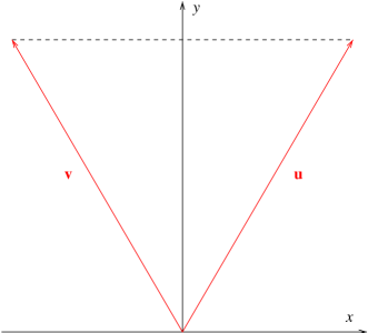
Figure 2: The coordinate system used to evaluate LISA’s transfer function.

As a concrete example of the general formalism described above we derive the sensitivity curve for the LISA interferometer using the design specifications quoted in the LISA Pre-Phase A Report[8]. Using the coordinate system shown in Figure 2, the unit vectors along each arm are given by

$${\bf u}=\frac{1}{2}\hat{x}+\frac{\sqrt{3}}{2}\hat{y}$$

$${\bf v}=-\frac{1}{2}\hat{x}+\frac{\sqrt{3}}{2}\hat{y}\,,$$ (35)

and the gravitational wave is described by

$$\widetilde{\Omega}=\cos\phi\,\sin\theta\,\hat{x}+\sin\phi\,\sin\theta\,\hat{y}+\cos\theta\,\hat{z}$$ (36)

$$\hat{m}=\sin\phi\,\hat{x}-\cos\phi\,\hat{y}$$ (37)

$$\hat{n}=\cos\phi\,\cos\theta\,\hat{x}+\sin\phi\,\cos\theta\,\hat{y}-\sin\theta\,\hat{z}\,.$$ (38)

The angle between the interferometer arms is ${\rm arccos}({\bf u}\cdot{\bf v})=\beta=\pi/3$. The various ingredients we need to calculate ${\cal R}(f)$ are

$${\bf u}\cdot\widehat{\Omega}=\sin(\phi+\pi/6)\sin\theta$$ (39)

$${\bf v}\cdot\widehat{\Omega}=\sin(\phi-\pi/6)\sin\theta$$ (40)

and

$$({\bf u}\otimes{\bf u}):{\bf e}^{+}=\frac{1}{4}\sin^{2}\theta+\frac{1}{2}\cos^{2}\theta\cos^{2}\phi-\frac{\sqrt{3}}{4}\sin 2\phi\,(1+\cos^{2}\theta)\,.$$ (41)

$$({\bf v}\otimes{\bf v}):{\bf e}^{+}=\frac{1}{4}\sin^{2}\theta+\frac{1}{2}\cos^{2}\theta\cos^{2}\phi+\frac{\sqrt{3}}{4}\sin 2\phi\,(1+\cos^{2}\theta)\,.$$ (42)

$$({\bf u}\otimes{\bf u}):{\bf e}^{\times}=-\cos\theta\sin(2\phi+\pi/3)\,.$$ (43)

$$({\bf v}\otimes{\bf v}):{\bf e}^{\times}=-\cos\theta\sin(2\phi-\pi/3)\,.$$ (44)

Before proceeding to find ${\cal R}(f)$ it is instructive to evaluate the detector response functions, $F^{A}(\widehat{\Omega},f)$, at zero frequency:

$$F^{+}(\widehat{\Omega}) = \frac{1}{2}({\bf u}\otimes{\bf u}-{\bf v}\otimes{\bf v}):{\bf e}^{+}$$ (45)

$$= -\frac{\sqrt{3}}{4}\sin 2\phi\,(1+\cos^{2}\theta)\,,$$

and

$$F^{\times}(\widehat{\Omega}) = \frac{1}{2}({\bf u}\otimes{\bf u}-{\bf v}\otimes{\bf v}):{\bf e}^{\times}$$ (46)

$$= -\frac{\sqrt{3}}{2}\cos 2\phi\,\cos\theta\,,$$

The magnitudes of these response functions are shown in Figure 3. They can be thought of as the polarization dependent antenna patterns for the LISA detector appropriate to a stochastic background of gravitational waves.

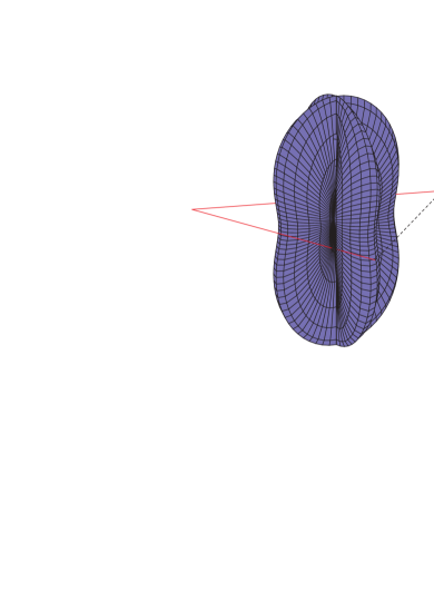
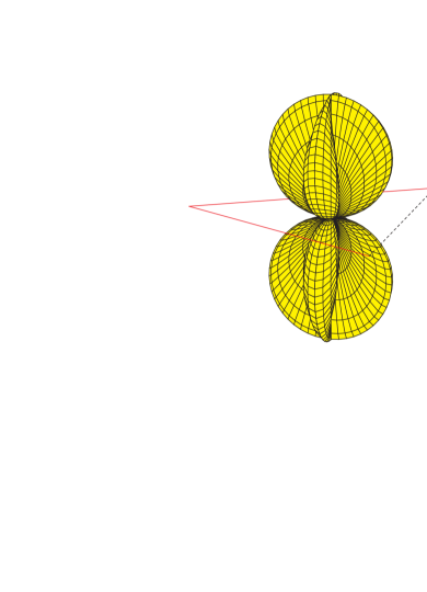
Figure 3: The magnitudes of the detector response functions $F^{+}(\widehat{\Omega},f)$ and $F^{\times}(\widehat{\Omega},f)$ in the low frequency limit.

Inserting equations (39) through (44) into equation (27) gives the transfer function ${\cal R}(f)$ in terms of an integral over the angles $\theta$ and $\phi$. Our explicit expression for LISA’s transfer function agrees with the one found by Larson, Hiscock and Hellings[20] using an alternative approach. We were unable to perform the angular integral to arrive at a general form for ${\cal R}(f)$, but for low frequencies the integrand can be expanded in a series to give

$${\cal R}(f)=\frac{2}{5}\sin^{2}\beta\left(1-\frac{37\cos^{2}(\beta/2)-10\cos^{4}(\beta/2)-1}{84\cos^{2}(\beta/2)}\left(\frac{f}{f_{*}}\right)^{2}\right.$$

$$+\left.\frac{20\cos^{6}(\beta/2)+163\cos^{2}(\beta/2)-80\cos^{4}(\beta/2)-6}{2268\cos^{2}(\beta/2)}\left(\frac{f}{f_{*}}\right)^{4}-\dots\right).$$ (47)

At frequencies above $f\sim\frac{3}{2}f_{*}$, the sinc function takes over and the transfer function falls of as $1/f^{2}$. Setting $\beta=\pi/3$, we find that a good approximation for the transfer function is given by

$${\cal R}(f)=\left\{\begin{array}[]{ll}{\displaystyle\frac{3}{10}\left(1-\frac{169}{504}\left(\frac{f}{f_{*}}\right)^{2}+\frac{425}{9072}\left(\frac{f}{f_{*}}\right)^{4}-\frac{165073}{47900160}\left(\frac{f}{f_{*}}\right)^{6}\right)},&f<\frac{3}{2}f_{*}\\ \>{\displaystyle\frac{16783143}{126156800}\left(\frac{3f_{*}}{2f}\right)^{2}},&f\geq\frac{3}{2}f_{*}\end{array}\right..$$ (48)

The coefficient in front of the high frequency term is chosen so that the transfer function is continuous at $f=\frac{3}{2}f_{*}$.

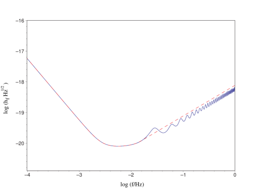
Figure 4: The effective noise floor for the LISA mission. The solid line was obtained numerically while the dashed line is our analytic approximation.

Now that we have calculated the transfer function, our next task is to estimate the the detector noise power, $S_{n}(f)$. There are many noise contributions discussed in the LISA Pre-Phase A Report[8]. The dominant ones are thought to be acceleration noise from the inertial sensors and position noise due to laser shot noise. A position noise of $\widetilde{\delta x}=2\times 10^{-11}$ m Hz^-1/2 is quoted for each LISA spacecraft. There are two such contributions per arm, giving a total of 4 contributions for the interferometer. Since the contributions are uncorrelated they add in quadrature to give a total position noise of $2\widetilde{\delta x}$. Dividing this by the optical path length of $2L$ and squaring gives the position noise power:

$$S_{n}^{\rm pos}(f)=\left(\frac{\widetilde{\delta x}}{L}\right)^{2}\;\,.$$ (49)

An acceleration noise of $\widetilde{\delta a}=3\times 10^{-15}$ ms^-2 Hz^-1/2 is quoted for each inertial sensor. This noise acts coherently on the incoming and outgoing signal, for a combined acceleration noise of $2\widetilde{\delta a}$ per spacecraft. There are four such contributions in the interferometer that add in quadrature for a total acceleration noise of $4\widetilde{\delta a}$. Dividing this by the square of the angular frequency of the gravitational wave yields the effective position noise due to spurious accelerations. Dividing the effective position noise by the optical path length and squaring gives the acceleration noise power:

$$S_{n}^{\rm accl}(f)=\left(\frac{2\widetilde{\delta a}}{(2\pi f)^{2}L}\right)^{2}\,.$$ (50)

Adding together the acceleration and position noise power gives the total noise power. Using the nominal values for the LISA mission[8] we obtain

$$S_{n}(f)=\left(9.24\times 10^{-40}\left(\frac{{\rm mHz}}{f}\right)^{4}+1.6\times 10^{-41}\right)\;{\rm Hz}^{-1}\,.$$ (51)

Inserting the above expression for $S_{n}(f)$, along with the approximate expression for the transfer function (48), into equation (34) yields a useful analytic approximation for the effective strain noise, $\tilde{h}_{\rm eff}(f)$, in the LISA interferometer. The analytic approximation is compared to the full numerical result in Figure 4.

LISA reaches a peak sensitivity in the frequency range $3\times 10^{-3}\rightarrow 10^{-2}$ Hz. Using equations (33) and (34) we have

$$S_{h}(f)=\tilde{h}_{\rm eff}^{2}(f)\,{\rm SNR}(f)\,.$$ (52)

For a SNR of 2, this translates into a sensitivity of

$$\tilde{h}_{\rm eff}(f)=6.2\times 10^{-21}\left(\frac{\Omega_{\rm gw}(f)h_{0}^{2}}{10^{-13}}\right)^{1/2}\left(\frac{f}{{\rm mHz}}\right)^{3/2}\,{\rm Hz}^{-1/2}\,.$$ (53)

Thus, a stochastic background with $\Omega_{\rm gw}(f)h_{0}^{2}>7\times 10^{-12}$ should dominate LISA’s instrument noise for frequencies near 3 mHz. The difficulty would come in deciding if the interferometer response was due to instrument noise or a stochastic background, as both are Gaussian random processes. One way to be sure is to fly two LISA interferometers and cross correlate their outputs.

4 Cross correlating two interferometers

Having demonstrated that our formalism recovers the standard results for a single interferometer, we now investigate how the sensitivity can be improved by cross correlating two interferometers. The most general form for the cross correlation of two detectors is given by

$$C = \int_{-T/2}^{T/2}dt\int_{-T/2}^{T/2}dt^{\prime}\,S_{1}(t)S_{2}(t^{\prime})Q(t-t^{\prime})$$ (54)

$$\simeq \int_{-\infty}^{\infty}df\int_{-\infty}^{\infty}df^{\prime}\delta_{T}(f-f^{\prime})\tilde{S}_{1}^{*}(f)\tilde{S}_{2}(f^{\prime})\widetilde{Q}(f^{\prime})\,.$$

Here $Q(t-t^{\prime})$ is a filter function and the $S_{i}$’s are the strain amplitudes that we read out from the $i^{\rm th}$ detector:

$$S_{i}(t)=h_{i}^{\rm astro}(t)+s_{i}(t)+n_{i}(t)\,.$$ (55)

The contributions are from resolvable astrophysical sources $h_{i}^{\rm astro}$, the stochastic background $s_{i}$, and intrinsic detector noise $n_{i}$. The function $\delta_{T}$ that appears in the Fourier space version of the correlation function is the “finite time delta function”

$$\delta_{T}=\int_{-T/2}^{T/2}dt\,e^{-2\pi ift}=\frac{\sin(\pi fT)}{\pi f}\,.$$ (56)

It obeys

$$\delta_{T}(0)=T\,\quad{\rm and}\quad\delta(x)=\lim_{T\rightarrow\infty}\delta_{T}(x)\,.$$ (57)

After removing resolvable astrophysical sources, the ensemble average of $C$ is given by

$$\langle C\rangle=\langle s_{1},s_{2}\rangle+\langle s_{1},n_{2}\rangle+\langle n_{1},s_{2}\rangle+\langle n_{1},n_{2}\rangle=\langle s_{1},s_{2}\rangle\,.$$ (58)

Notice that terms involving the noise vanish as the noise is uncorrelated with the signal, and the noise in different detectors is also uncorrelated. Thus,

$$\langle C\rangle=\langle s_{1},s_{2}\rangle=\int_{-\infty}^{\infty}df\int_{-\infty}^{\infty}df^{\prime}\delta_{T}(f-f^{\prime})\langle\tilde{s}_{1}^{*}(f)\tilde{s}_{2}(f^{\prime})\rangle\,\widetilde{Q}(f^{\prime})\,.$$ (59)

Our next task is to evaluate the quantity $\langle\tilde{s}_{1}^{*}(f)\tilde{s}_{2}(f^{\prime})\rangle$ that appears in equation (59). Taking the Fourier transform of the expression in (14) and performing the ensemble average we find

$$\langle\tilde{s}_{1}^{*}(f)\tilde{s}_{2}(f^{\prime})\rangle=\frac{1}{2}\delta(f-f^{\prime})S_{h}(f)\,\gamma(f)\,\frac{2}{5}\sin^{2}\beta\,,$$ (60)

where $\gamma(f)$ is the overlap reduction function

$$\gamma(f)=\frac{5}{2\sin^{2}\beta}\int\frac{d\widehat{\Omega}}{4\pi}\left({F_{1}^{+}}^{*}(\widehat{\Omega},f)F_{2}^{+}(\widehat{\Omega},f)+{F_{1}^{\times}}^{*}(\widehat{\Omega},f)F_{2}^{\times}(\widehat{\Omega},f)\right)e^{-2\pi if\widehat{\Omega}\cdot({\bf x}_{1}-{\bf x}_{2})/c}\,.$$ (61)

The normalization is chosen so that $\gamma(0)=1$. The function $\gamma(f)$ is Hermitian in the sense that $\gamma_{12}(f)=\gamma^{*}_{21}(f)$. The inverse Fourier transform of $\gamma(f)$ is a real function since $\gamma^{*}(f)=\gamma(-f)$. The term “overlap reduction function” refers to the fact that $\gamma(f)$ takes into account the misalignment and separation of the interferometers. In addition, $\gamma(f)$ contains the transfer functions for each detector, as can be seen by setting $F_{1}=F_{2}$ in (61) and comparing with (27):

$$\gamma_{1=2}(f)=\frac{5}{2\sin^{2}\beta}\;{\cal R}(f)\,.$$ (62)

In other words, $\gamma(f)$ is an overlap reduction function and detector transfer function all rolled into one. Inserting equation (60) into equation (59) yields the expectation value of $C$:

$$\langle C\rangle = \frac{T}{5}\sin^{2}\beta\,\int^{\infty}_{-\infty}df\,S_{h}(f)\gamma(f)\widetilde{Q}(f)$$ (63)

$$= \frac{2T}{5}\sin^{2}\beta\,\int^{\infty}_{0}df\,S_{h}(f)\Re[\gamma(f)\widetilde{Q}(f)]\,.$$

In the final line we have switched from the mathematically convenient range of integration $f\in(-\infty,\infty)$ to the physically relevant range $f\in[0,\infty)$.

The noise in a measurement of $C$ is given by $N=C-\langle C\rangle$, and the signal to noise ratio (squared) is given by

$${\rm SNR}^{2}\equiv\frac{\langle C\rangle^{2}}{\langle N^{2}\rangle}=\frac{\langle C\rangle^{2}}{\langle C^{2}\rangle-\langle C\rangle^{2}}\,.$$ (64)

Our task is to find the filter function $\widetilde{Q}(f)$ that maximizes this signal to noise ratio. A lengthy but straightforward calculation yields

$${\langle N^{2}\rangle}=\frac{T}{4}\int_{-\infty}^{\infty}|\widetilde{Q}(f)|^{2}M(f)\,df\,.$$ (65)

where

$$M(f) = S_{n1}(f)\,S_{n2}(f)+S_{n1}(f)S_{h}(f){\cal R}_{2}(f)+S_{n2}(f)S_{h}(f){\cal R}_{1}(f)$$ (66)

$$\hskip 72.26999pt+S_{h}^{2}(f)\left(|\gamma(f)|^{2}+\frac{{\cal R}_{1}(f){\cal R}_{2}(f)}{(2/5\,\sin^{2}\beta)^{2}}\right)\,.$$

Here $S_{n,i}$ and ${\cal R}_{i}$ denote the spectral noise and the transfer function for the $i^{\rm th}$ interferometer. The square of the signal to noise ratio can be written as

$${\rm SNR}^{2}=\frac{8T}{25}\sin^{4}\beta\;\frac{\{\widetilde{P},\widetilde{Q}\}^{2}}{\{\widetilde{Q},\widetilde{Q}\}}\,,$$ (67)

where $\{A,B\}$ denotes the inner product[15]

$$\{A,B\}=\int_{-\infty}^{\infty}df\,A^{*}(f)B(f)M(f)\,,$$ (68)

and

$$\widetilde{P}(f)=\frac{S_{h}(f)\gamma^{*}(f)}{M(f)}\,.$$ (69)

The signal to noise ratio is maximized by choosing the optimal filter “parallel” to $\widetilde{P}$. Since the normalization of $\widetilde{Q}$ drops out, we set $\widetilde{Q}(f)=\widetilde{P}(f)$[14, 15]. Using this filter, the optimal signal to noise ratio for the cross correlated interferometers is given by

$${\rm SNR}^{2}=\frac{8T}{25}\sin^{4}\beta\int_{0}^{\infty}df\frac{|\gamma(f)|^{2}S_{h}^{2}(f)}{M(f)}\,,$$ (70)

or, equivalently, as

$${\rm SNR}^{2}=\frac{9H_{0}^{4}\sin^{4}\beta}{50\pi^{4}}\,T\int_{0}^{\infty}df\frac{|\gamma(f)|^{2}\,\Omega_{{\rm gw}}^{2}(f)}{f^{6}M(f)}\,.$$ (71)

In the limit that the noise power in each interferometer is very much larger than the signal power we find

$${\rm SNR}^{2}=\frac{9H_{0}^{4}\sin^{4}\beta}{50\pi^{4}}\,T\int_{0}^{\infty}df\frac{|\gamma(f)|^{2}\,\Omega_{{\rm gw}}^{2}(f)}{f^{6}S_{n1}(f)S_{n2}(f)}\,,$$ (72)

which recovers the expressions quoted by Flanagan[14] and Allen[15] when we set $\beta=\pi/2$. The factor of $\sin^{4}\beta$ was missed in these papers, as the implicit assumption that $\beta=\pi/2$ crept into supposedly general expressions. The main new ingredient in our expression are the transfer functions ${\cal T}_{i}(f)$ that reside in the overlap reduction function $\gamma(f)$. The transfer functions prevent us from performing the integral over the two-sphere in equation (61) in closed form except at low frequency. However, it is a simple matter to numerically evaluate $\gamma(f)$ for a given detector configuration.

If we are trying to detect a weak stochastic background with a noisy detector, then equation (72) is the appropriate expression to use for the SNR. However, there may be some range of frequencies where the signal power dominates the noise power in each detector. The contribution to the SNR from a clean frequency window of this sort is given by

$${\rm SNR}^{2}(f,\Delta f)=T\,\frac{8\sin^{4}\beta}{25}\int_{f-\Delta f/2}^{f+\Delta f/2}df^{\prime}\,\frac{|\gamma(f^{\prime})|^{2}}{\left(|\gamma(f^{\prime})|^{2}+{\cal R}_{1}(f^{\prime}){\cal R}_{2}(f^{\prime})/(2/5\,\sin^{2}\beta)^{2}\right)}\,.$$ (73)

The integrand is approximately equal to $1/2$ for all frequencies, so that

$${\rm SNR}(f,\Delta f)\simeq\frac{2}{5}\sin^{2}\beta\,\sqrt{T\Delta f}\,.$$ (74)

This expression provides a useful lower bound for the SNR that can be achieved for detectors with a clean frequency window of width $\Delta f$ centered at some frequency $f$. For example, the spectral density due to white dwarf binaries in our galaxy is expected to exceed LISA’s noise spectral density for frequencies in the range $10^{-4}\rightarrow 3\times 10^{-3}$ Hz. To detect this background at 90% confidence requires a signal to noise ratio of SNR=1.65, which can be achieved with less than three hours of integration time $T$.

4.1 Cross correlating two LISA interferometers

One possible modification to the current LISA proposal[8] would be to fly six spacecraft instead of three, and thereby form two independent interferometers. The cost of doing this is considerably less than twice the cost of the current proposal, and it has the advantage of providing additional redundancy to the mission. How would we best use a pair of LISA interferometers? If our main concern is getting better positional information on bright astrophysical sources, then we would fly the two interferometers far apart, eg. with one leading and the other trailing the Earth. However, if we want to maximize the cross correlation then we need the interferometers to be coincident and coaligned. However, a configuration of this type is likely to share correlated noise sources, which would defeat the purpose of cross correlating the interferometers. A better choice is to use a configuration that is coaligned but not coincident. This can be done by placing six spacecraft at the corners of a regular hexagon as shown in Figure 5. Notice that interferometers have parallel arms and that the corner spacecraft are separated by the diameter of the circle.

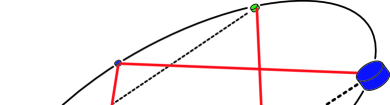
Figure 5: The hexagonal cross correlation pattern.

Using the same coordinate system that we used earlier for a single interferometer, the unit vectors ${\bf u}_{i}$ and ${\bf v}_{i}$ along each interferometer arm are:

$${\bf u}_{1}=-{\bf u}_{2}=\frac{1}{2}\hat{x}+\frac{\sqrt{3}}{2}\hat{y}$$

$${\bf v}_{1}=-{\bf v}_{2}=-\frac{1}{2}\hat{x}+\frac{\sqrt{3}}{2}\hat{y}\,,$$ (75)

where the index $i=1,2$ labels the two interferometers. The displacement of the corner spacecraft is given by

$${\bf x}_{1}-{\bf x}_{2}=-2R\,\hat{y}$$ (76)

where $R$ is the radius of the orbit. The angle between the interferometer arms is $\beta=\pi/3$, and the length of each arm is $L=\sqrt{3}R$. The light crossing time between the two interferometers, $2R/c$, is almost equal to the light crossing time along each interferometer arm, $\sqrt{3}R/c$. Thus, the loss of sensitivity due to multiple wavelengths fitting between the interferometers occurs for frequencies near the transfer frequency $f_{*}$ (the transfer frequency corresponds to wavelengths that fit inside the interferometer arms). For LISA the transfer frequency is $f_{*}=9.54\times 10^{-3}$ Hz.

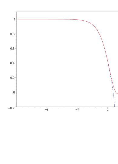
Figure 6: The overlap reduction function for the hexagonal cross correlation patern. The solid line was generated numerically while the dashed line is our analytic approximation from equation (77).

The various ingredients we need to calculate $\gamma(f)$ follow from those given in equations (39) through (44). Putting everything together in (61) and working in the low frequency limit we find

$$\gamma(f)=1-\frac{383}{504}\left(\frac{f}{f_{*}}\right)^{2}+\frac{893}{3888}\left(\frac{f}{f_{*}}\right)^{4}-\frac{5414989}{143700480}\left(\frac{f}{f_{*}}\right)^{6}+\dots$$ (77)

For frequencies above $f_{*}$ the overlap reduction function decays as $f^{-2}$. A numerically generated plot of $\gamma(f)$ is displayed in Figure 6. Scaling the signal to noise ratio (72) in units appropriate to a pair of LISA interferometers we have

$${\rm SNR}^{2}=34.4\left(\frac{T}{{\rm year}}\right)\int_{0}^{\infty}\left(\frac{df}{{\rm mHz}}\right)\,|\gamma(f)|^{2}\left(\frac{\Omega_{{\rm gw}}(f)h_{0}^{2}}{10^{-15}}\right)^{2}\left(\frac{{\rm mHz}}{f}\right)^{6}\left(\frac{10^{-41}\,{\rm Hz}^{-1}}{S_{n}(f)}\right)^{2}\,.$$ (78)

Using equation (51) for $S_{n}(f)$ and assuming a scale invariant stochastic background yields a signal to noise of

$${\rm SNR}=1.44\sqrt{\frac{T}{{\rm year}}}\left(\frac{\Omega_{{\rm gw}}h_{0}^{2}}{10^{-14}}\right)\,.$$ (79)

This represents a 500 fold improvement on the sensitivity of a single LISA detector. Indeed, if it were not for the astrophysical foregrounds, a pair of LISA detectors would be well poised to detect a scale invariant gravitational wave background from inflation.

5 Missions to detect the CGB

We will work on the assumption that astrophysical foregrounds swamp the CGB for frequencies above a few $\mu$Hz, and design our missions accordingly. What we have in mind is a post-LISA mission based on the (by then) tried and tested LISA technology, but with some allowance for improvements in basic technologies such as the accelerometers. Since cross-correlating two interferometers at ultra-low frequencies does not buy us a major improvement in sensitivity, we need to start with a design that has excellent sensitivity at low frequencies. Basically this means building bigger interferometers with better accelerometers. To be concrete, we show the sensitivity curves for three generations of LISA missions in Figure 7. LISA I corresponds to the current LISA design with the spacecraft cart-wheeling about the Sun at 1 AU, separated by $L=5\times 10^{9}$ m. LISA II refers to a possible follow on mission with the three spacecraft evenly spaced around an orbit at 1 AU, so that the spacecraft are separated by $L=\sqrt{3}$ AU. The LISA II mission would use similar optics to LISA I (same laser power and telescope size), but allows for an order of magnitude improvement in accelerometer performance. LISA III is similar to LISA II, except that the constellation would orbit at 35 AU (between Neptune and Pluto) and the accelerometers would be improved by a further two orders of magnitude. The acceleration noise for LISA III would benefit from the three orders of magnitude reduction in solar radiation relative to LISAs I and II, but this would come at the cost of having to power the spacecraft using nuclear generators (RTGs).

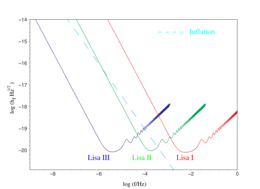
Figure 7: Sensitivity curves for three generations of LISA missions. Also shown is a prediction for the CGB in a scale invariant inflationary scenario.

For all three missions we see that the $\mu$Hz range lies well below the interferometer’s transfer frequency

$$f_{*}=1.84\times 10^{-4}\left(\frac{\sqrt{3}\,{\rm AU}}{L}\right)\;{\rm Hz}\,.$$ (80)

Indeed, it would take a mission orbiting at 180 AU ( somewhere inside the Kuiper belt) to achieve a transfer frequency of $f_{*}=10^{-6}$ Hz. In practical terms this allows us to work in the low frequency limit $f\ll f_{*}$ where it is easy to derive analytic expressions for the overlap reduction function $\gamma(f)$. Moreover, we need only consider acceleration noise when working below 1$\mu$Hz. All our calculations are based on the same hexagonal cross correlation shown in Figure 5 that we used for the LISA I cross correlation. Using equation (50) for the acceleration noise and ignoring the position noise yields

$$S_{n}(f)=3.42\times 10^{-33}\left(\frac{\sqrt{3}\,{\rm AU}}{L}\right)^{2}\left(\frac{\mu{\rm Hz}}{f}\right)^{4}\left(\frac{\delta a}{3\times 10^{-16}{\rm m}{\rm s}^{-2}}\right)^{2}\,{\rm Hz}^{-1}.$$ (81)

In the limit that the noise power dominates the spectral density of the CGB we arrive at an estimate for the signal to noise ratio for frequencies below 1$\mu$Hz

$${\rm SNR}^{2} = 29.4\left(\frac{T}{{\rm year}}\right)\left(\frac{L}{\sqrt{3}\,{\rm AU}}\right)^{4}\left(\frac{3\times 10^{-16}{\rm m}{\rm s}^{-2}}{\delta a}\right)^{4}\times$$

$$\quad\int_{0}^{f}|\gamma(f^{\prime})|^{2}\left(\frac{\Omega_{\rm gw}(f^{\prime})h_{0}^{2}}{10^{-14}}\right)^{2}\left(\frac{f^{\prime}}{\mu{\rm Hz}}\right)^{2}\left(\frac{df^{\prime}}{\mu{\rm Hz}}\right)\,.$$ (82)

The SNR is scaled against the LISA II specifications. Since $f/f_{*}\ll 1$ it is a good approximation to set $\gamma(f)=1$ inside the integral. We model the CGB spectrum near 1$\mu$Hz by a simple power law:

$$\Omega_{\rm gw}(f)=\Omega_{\mu{\rm Hz}}\left(\frac{f}{\mu{\rm Hz}}\right)^{\alpha}\,,$$ (83)

scaled relative to a reference value at 1$\mu$Hz. With these approximations we arrive at our final expression for the SNR for a pair of cross correlated interferometers in the ultra low frequency regime:

$${\rm SNR}=\frac{3.13}{\sqrt{1+2\alpha/3}}\left(\frac{T}{{\rm year}}\right)^{1/2}\left(\frac{L}{\sqrt{3}\,{\rm AU}}\right)^{2}\left(\frac{3\times 10^{-16}{\rm m}{\rm s}^{-2}}{\delta a}\right)^{2}\left(\frac{\Omega_{\mu{\rm Hz}}\,h_{0}^{2}}{10^{-14}}\right)\left(\frac{f}{\mu{\rm Hz}}\right)^{\alpha+3/2}$$

(84)

We can compare this to the SNR of a single interferometer in the ultra low frequency regime by combining equations (23), (33) and (81) to find

$${\rm SNR}_{s}(f)=0.683\left(\frac{L}{\sqrt{3}\,{\rm AU}}\right)^{2}\left(\frac{3\times 10^{-16}{\rm m}{\rm s}^{-2}}{\delta a}\right)^{2}\left(\frac{\Omega_{\mu{\rm Hz}}\,h_{0}^{2}}{10^{-14}}\right)\left(\frac{f}{\mu{\rm Hz}}\right)^{\alpha+1}\,.$$ (85)

We see that the individual and cross correlated sensitivities are related:

$${\rm SNR}=\frac{0.82}{\sqrt{1+2\alpha/3}}\,(T\Delta f)^{1/2}\;{\rm SNR}_{s}(f)\,,\quad{\rm for}\;f\approx\Delta f\approx 1\,\mu{\rm Hz}\,.$$ (86)

This supports our earlier assertion that cross correlating two interferometers improves on the sensitivity of a single interferometer by $(T\Delta f)^{1/2}$ where $\Delta f$ is approximately equal to the central observing frequency $f$.

Equation (5) tells us that a GABI detector built from two LISA II interferometers could detect the CGB at greater than 90% confidence with one year of data taking if $\Omega_{\rm gw}(1\mu{\rm Hz})h_{0}^{2}=10^{-14}$. The same equation also tells us what has to be done to achieve greater sensitivity. It is clear that increasing the duration of the mission is not the best answer as the SNR only improves as the square root of the observation time. In contrast, increasing the size of the interferometer or reducing the acceleration noise produces a quadratic increase in sensitivity. For example, a GABI detector built from a pair of LISA III interferometers could detect the CGB at 90% confidence for signals as small as $\Omega_{\rm gw}(1\mu{\rm Hz})h_{0}^{2}=4\times 10^{-22}$. In-fact, for signal strengths above this value the LISA III detectors are signal dominated and we need to use equation (74) instead of (5) to calculate the SNR.

We can also use equation (5) to determine how well a GABI mission can measure the CGB power spectrum. Suppose that we break up the frequency spectrum into bins of width $\delta f$. Nyquist’s theorem tells us that $\delta f\geq 1/T$, eg. for an observation time of one year the frequency resolution is $3.17\times 10^{-8}$ Hz. Writing $\delta f=n/T$ where $n\geq 1$, and taking $\delta f\ll f$, we find from (5) that in the frequency window $(f-\delta f/2,f+\delta f/2)$ the SNR is

$${\rm SNR}(f,\delta f)=0.965\sqrt{n}\left(\frac{L}{\sqrt{3}\,{\rm AU}}\right)^{2}\left(\frac{3\times 10^{-16}{\rm m}{\rm s}^{-2}}{\delta a}\right)^{2}\left(\frac{\Omega_{\mu{\rm Hz}}\,h_{0}^{2}}{10^{-14}}\right)\left(\frac{f}{\mu{\rm Hz}}\right)^{\alpha+1}\,.$$ (87)

We see that the SNR in each frequency bin scales as $f^{1+\alpha}$. For a scale invariant spectrum ($\alpha=0$) this translates into poor performance at frequencies below 1 $\mu$Hz and limits the range over which we can measure the spectrum. For example, if the CGB has a scale invariant spectrum and an amplitude of $\Omega_{{\rm gw}}h_{0}^{2}\geq 2\times 10^{-13}$, a pair of LISA II interferometers could measure the spectrum over the range $10^{-7}\rightarrow 10^{-6}$ Hz. For a pair of LISA III detectors the main limitation at low frequencies comes from Nyquist’s theorem. Since mission lifetimes are limited to tens of years, it will not be possible to measure the CGB spectrum much below $10^{-8}$ Hz using space based interferometers. Indeed, it may be difficult to push much below $10^{-7}$ Hz unless ways can be found to build detectors that are stable for many months. A pair of LISA III interferometers could measure the spectrum between $10^{-8}\rightarrow 10^{-6}$ Hz if $\Omega_{{\rm gw}}(10^{-8}\,{\rm Hz})h_{0}^{2}\geq 10^{-18}$. To measure the CGB spectrum below $10^{-8}$ Hz requires a return, full circle, to the world of CMB physics. Detailed polarization measurements of the CMB can be used to infer[21] the CGB power spectrum for frequencies in the range $10^{-18}\rightarrow 10^{-16}$ Hz.

6 Discussion

The LISA follow-on missions we have described will be able to detect or place stringent bounds on the CGB amplitude and spectrum between $10^{-8}$ and $10^{-6}$ Hz. But how can we be sure that it is the CGB we have detected and not some unresolved astrophysical foreground? The answer can be found in the statistical character of the competing signals. Most early universe theories predict that the CGB is truly stochastic. In contrast, the astrophysical signal is only approximately stochastic, in a sense that can be made precise by appealing to the central limit theorem. The line in Figure 1 indicating the predicted amplitude of various astrophysical foregrounds corresponds to what is known as the confusion limit. It marks the amplitude at which we can expect to find, on average, one source per frequency bin. It is not until we reach signal strengths considerably smaller than the confusion limit that the astrophysical signal starts to look stochastic. And therein lies the answer to our question. A “stochastic” signal due to astrophysical sources will always have bright outliers that sit just above the amplitude of the stochastic signal. The number and distribution of the outliers can be predicted on statistical grounds. If we do not see the outliers, then we can safely conclude that we have detected the CGB.

References

References

- [1] de Bernardis P et al. 2000 Nature 404 955.
- [2] Balbi A et al. 2000 Astrophys. J. 545 L1.
- [3] Bennett C L et al. 1996 Astrophys. J. 464 L1.
- [4] Mather J C et al. 1990 Astrophys. J. 354 L37.
- [5] Cornish N J & Larson S L 2001 in preparation
- [6] Hogan, C J 2000 Phys. Rev. Lett.85, 2044.
- [7] Riazuelo A & Uzan J-P 2000 Phys. Rev.D62 083506.
- [8] Bender P et al. 1998 LISA Pre-Phase A Report.
- [9] Schneider R, Ferrara A, Ciardi B, Ferrari V & Matarrese S 2000 Mon. Not. Roy. Astron. Soc. 317, 365; Schneider R, Ferrari V, Matarrese S & Portegies Zwart S F 2000 Mon. Not. Roy. Astron. Soc..
- [10] Maggiore M 2000 Phys. Rep. 331, 283.
- [11] Tinto M, Armstrong J W & Estabrook F B 2001 Phys. Rev.D63, 021101(R).
- [12] Michelson P F 1987 Mon. Not. Roy. Astron. Soc. 227, 933.
- [13] Christensen N 1992 Phys. Rev.D46, 5250.
- [14] Flanagan E E 1993 Phys. Rev.D48, 2389.
- [15] Allen B 1996 Proceedings of the Les Houches School on Astrophysical Sources of Gravitational Waves eds. Marck J-A and Lasota J-P (Cambridge: Cambridge University Press) p 373
- [16] Allen B & Romano J D 1999 Phys. Rev.D59, 102001.
- [17] Hellings R W 1983 Gravitational Radiation eds. Dereulle N and Piran T (Amsterdam: North Holland) p 485.
- [18] Schilling R 1997 Class. Quantum Grav.14, 1513.
- [19] Armstrong J W, Estabrook F B & Tinto M 1999 Astrophys. J. 527, 814.
- [20] Larson S L, Hiscock W A & Hellings R W 2000 Phys. Rev.D62, 062001.
- [21] Caldwell R R, Kamionkowski M & Wadley L 1999 Phys. Rev.D59, 027101.