Late-time dynamics of rapidly rotating black holes

Abstract

We study the late-time behaviour of a dynamically perturbed rapidly rotating black hole. Considering an extreme Kerr black hole, we show that the large number of virtually undamped quasinormal modes (that exist for nonzero values of the azimuthal eigenvalue $m$) combine in such a way that the field (as observed at infinity) oscillates with an amplitude that decays as $1/t$ at late times. This is in clear contrast with the standard late time power-law fall-off familiar from studies of non-rotating black holes. This long-lived oscillating “tail” will, however, not be present for non-extreme (presumably more astrophysically relevant) black holes, for which we find that many quasinormal modes (individually excited to a very small amplitude) combine to give rise to an exponentially decaying field. This result could have implications for the detection of gravitational-wave signals from rapidly spinning black holes, since the required theoretical templates need to be constructed from linear combinations of many modes. Our main results are obtained analytically, but we support the conclusions with numerical time-evolutions of the Teukolsky equation. These time-evolutions provide an interesting insight into the notion that the quasinormal modes can be viewed as waves trapped in the spacetime region outside the horizon. They also suggest that a plausible mechanism for the behaviour we observe for extreme black holes is the presence of a “superradiance resonance cavity” immediately outside the black hole.

I Introduction

I.1 A brief background

The generic response of a black hole to dynamical perturbations was first investigated more than thirty years ago. Vishveshwara vishu was the first to observe, in simple numerical experiments where a Schwarzschild black hole was pelted by Gaussian wave-pulses, the “ringing” associated with the exponentially damped quasinormal modes (QNMs). Shortly thereafter, the late time power-law fall-off (that all perturbative fields decay as $t^{-2l-3}$ in the Schwarzschild geometry) was discovered by Price price . Since these first studies, a considerable body of work has established the importance of these two phenomena for black hole physics (see novikov for a review).

We now know that the late-time tail is due to radiation backscattered by the weak gravitational potential in the far-zoneGPP . It is independent of the central object’s strong-field features (such as the presence of an event horizon), and will consequently be the same for (say) a neutron star and a black hole with the same gravitational mass. In contrast, the QNMs represent radiation scattered in the strong-field regime. Hence, they provide the means for making a clear distinction between a neutron star and a black hole. A neutron star has many families of fluid pulsations modes, an observation of which would provide useful constraints on the supranuclear equation of state astero . In addition, there is a set of modes that arise because gravitational waves can be temporarily trapped by the spacetime curvature caused by the presence of the star. These modes share some qualitative features with the QNMs of a black hole, which arise as waves are temporarily trapped in the vicinity of the black hole’s gravitational potential peak (located near the unstable photon orbit at $r=3M$ in the Schwarzschild case). The modes are analogous to scattering resonances in quantum physics and thus decay exponentially in time. In a detailed study, Leaver leaver1 identified the QNMs as complex-frequency poles of the relevant Green’s function (see also na ). In addition, he showed that the power-law tail, that dominates the black holes dynamical response once the QNMs have died away, originates from the presence of a branch cut in the Green’s function (customarily placed along the negative imaginary frequency axis).

Most previous studies of QNMs and power-law tails have focused on non-rotating black holes, and our understanding of this case has reached a mature level. The same can not be said about the rotating case, however. A few years ago, the QNMs had been calculated also for Kerr black holes leaver2 ; onozawa , but there were no actual calculations demonstrating the presence of power-law tails. Several recent developments have improved our understanding of dynamical rotating black holes. Of particular relevance has been an effort to develop a reliable framework for perturbative time-evolutions of Kerr black holes tcode1 ; tcode2 ; tcode3 ; tcode4 . There has also been recent efforts to analytically approximate the late-time power-law tails for Kerr black holes hod ; barack1 ; barack2 . The main conclusions of these studies support the standard picture: The QNM signal (typically dominated by the slowest damped mode) gives way at late times to a power-law fall-off. Although the QNM frequencies and the late-time power-law are slightly altered by rotation, the results are qualitatively similar to the Schwarzschild ones. For example, for a massless scalar field Ori and Barack barack1 ; barack2 predict a fall-off (for non-extreme Kerr black holes) proportional to $t^{-l-|m|-3-q}$ where $q=0/1$ for even/odd $l+m$. This should be compared to the Schwarzschild result $t^{-2l-3}$. The difference can be attributed to the rotation-induced coupling of the various $l$-multipoles in the signal.

I.2 Motivation: The observability of QNM signals

With a new generation of gravitational-wave detectors due to reach their projected sensitivities within the next few years, the question whether we can realistically hope to do “black-hole spectroscopy” by detecting QNM signals following (say) the formation of a black hole in a supernova is of obvious interest. In principle, such a detection should enable us to infer the black-hole mass and angular momemtum and therefore provide an unambiguous identification of astrophysical black holes.

For slowly rotating black holes this presents a serious challenge. To demonstrate this in a simple way we consider the gravitational wave signal associated with a certain QNM. Far away from the black hole the associated flux follows from the standard formula

$$F={1\over 16\pi}|\dot{h}|^{2}={1\over 4\pi r^{2}}{dE\over dt}.$$ (1)

Using this together with

$${dE\over dt}={E\over 2\tau_{e}}$$ (2)

where $\tau_{e}$ is the e-folding time of the QNM, and assuming a monochromatic wave (of frequency $f$) such that $\dot{h}=2\pi fh$ (although we note that this assumption is not justified for rapidly damped QNMs), we get

$$h=\left({E\over\tau_{e}}\right)^{1/2}{1\over\pi rf}$$ (3)

Finally, we estimate the effective amplitude achievable after matched filtering as

$$h_{\rm eff}=h\sqrt{N}=h\sqrt{f\tau_{e}}$$ (4)

where $N$ is the number of detected cycles of the signal. Parameterising this result we arrive at (cf. similar estimates for pulsating stars astero )

$$h_{\rm eff}\approx 4.2\times 10^{-24}\left({\delta\over 10^{-6}}\right)^{1/2}\left({M\over M_{\odot}}\right)\left({15{\rm Mpc}\over r}\right)$$ (5)

where $\delta$ is the radiated energy as a fraction of the black hole’s mass $M$. For a Schwarzschild black hole the frequency of the radiation depends on the black-hole mass as $f\approx 12({M_{\odot}/M}){\rm kHz}$. Given these relations, and recalling the estimated sensitivity of the generation of ground based detectors that is under construction (LIGO, VIRGO, GEO600 and TAMA), we see that it is going to be difficult to see QNM signals from slowly rotating solar-mass black holes. The mode-signals are basically too rapidly damped. But there are reasons not to despair. First of all, the situation is much more favourable for low-frequency signals from supramassive black holes in galactic nuclei and detection with LISA, the space-based interferometric gravitational-wave antenna. Secondly, there have been recent indications that “middle weight” black holes, with masses in the range $100-1000M_{\odot}$, exist mediumbh1 ; mediumbh2 . For such black holes the most important QNMs would radiate at frequencies where the new generation of ground based detectors reach their peak sensitivity ($\sim 100$ Hz). If there are such black holes in our galaxy, and they are dynamically perturbed by some external agent, we may hope to detect the resultant QNM ringing in the future.

It has been suggested that QNM signals from rapidly rotating black holes would be easier to detect than what the above estimate suggests. This belief is based on the fact that some QNMs become very long lived as $a\to M$ (where $0\leq a\leq M$ is the rotation parameter of the black hole). QNM calculations predict the existence of an infinite set of essentially undamped modes in the extreme Kerr limit leaver2 ; onozawa ; detweiler , and previous investigations into the detectability of QNM signals have focused on the slow damping of these modes echeverria ; finn ; flanagan . It is easy to see how the decreased damping of the modes may increase the detectability considerably. But it is also easy to understand that a slowly damped mode is only easier to detect than a short-lived one if the modes are excited to a comparable amplitude. This then forces us to address (rather difficult) issues regarding QNM excitation na ; nollert . In particular, we must investigate whether it is easier to excite a slowly damped QNM than a short-lived one. Intuitively, one might expect this not to be the case. In similar physical situations the build-up of energy in a long-lived resonant mode takes place on a time-scale similar to the eventual mode damping. Consequently, it ought to be quite difficult to excite a QNM that has characteristic damping several times longer than the dynamical timescale of the excitation process. This argument suggests that the amplitude of each long-lived mode ought to vanish in the limit $a\to M$ when the e-folding time of the mode increases dramatically. Indications that this is the case were provided by Ferrari and Mashhoon some years ago ferrari .

To illustrate this further, we connect (4) to the amplitude of the QNM under consideration. We do this by assuming that the mode-signal can be represented by

$$h\approx{Ae^{-t/\tau_{e}}\over r}\sin(2\pi ft)\ .$$ (6)

Then we can use (3) to infer the “amplitude” $A$ that corresponds to a certain “total energy radiated through the mode” $E$. We get

$$E={\pi^{2}f^{2}\tau_{e}\over 4}A^{2}\ ,$$ (7)

and the effective gravitational-wave amplitude

$$h_{\rm eff}={\sqrt{f\tau_{e}}\over 2}A\approx\left(1-{a\over M}\right)^{-3/10}{A\over\sqrt{2\pi}}\ .$$ (8)

Here we have used an empirical approximation for the frequency and damping rate of the fundamental $l=m=2$ mode echeverria . When the effective amplitude is expressed in this form it is quite clear that a decrease in $A$ can easily compensate for the increase in $\tau_{e}$ that occurs as the black hole spins up. In other words, in order to correctly discuss the detectability of the Kerr QNMs one must necessarily investigate this balance. This provides the prime motivation for the present work.

I.3 A brief summary of previous work

In a previous paper prl we discussed some issues concerning the long-lived QNMs of a Kerr black hole. Our results essentially followed by studying a suitably defined excitation coefficient (defined in terms of the asymptotic behaviour of the perturbed field, see Section IIE of the present paper), $A^{\rm out}/\alpha_{n}$. Provided that one can calculate this quantity (which is far from trivial na ) for a given QNM as the black hole spin varies one can estimate the associated change in level of excitation of the mode. This follows since we can express the effective amplitude (8) associated with a single QNM (with complex frequency $\omega_{n}$) as

$$h_{\rm eff}=\frac{\sqrt{f\tau_{e}}}{2}A\sim\sqrt{{\mbox{Re }\omega_{n}\over\mbox{Im }\omega_{n}}}{A^{\rm out}\over\alpha_{n}}\ .$$ (9)

Using results derived in the main part of this paper we find, for an extreme Kerr black hole, that

$$h_{\rm eff}\sim e^{-n\pi/2\delta}$$ (10)

where $\delta$ is a positive real constant (see Section IID for its definition), and the least damped modes correspond to large values of the integer $n$. From this we immediately deduce that the “effective detectability” is exponentially small for these modes.

Similar evidence is provided by recently obtained numerical data modepaper relevant for the full range of $a$. Before we discuss these results we recall that the QNMs of a non-rotating black hole are located symmetrically with respect to the imaginary frequency axis in the complex $\omega$-plane. For non-zero $a$ this symmetry is broken and co- and counter-rotating modes will be affected in different ways. The counter-rotating modes remain rapidly damped, while the co-rotating modes become very slowly damped as $a\to M$. These conclusions follow from eg. Figure 3 in leaver2 .

In Figure  1 we compare the “effective gravitational-wave amplitude” obtained from (9) for the slowest damped co- and counter-rotating QNMs of a Kerr black hole perturbed by a massless scalar field. From the figure we see that, even though the co-rotating mode is much longer lived, its “detectability” decreases significantly as $a\to M$. In fact, our results suggest that the effective amplitude of the slowest damped QNM for a rapidly rotating black hole may be as much as three orders of magnitude smaller than the amplitude of the corresponding mode of a Schwarzschild black hole. This is clearly very bad news as far as detecting the various QNMs of a rapidly spinning black hole is concerned.

Figure 1: An assessment of the “detectability” of Kerr black hole QNMs as $a\to M$. The effective amplitude $h_{\rm eff}$ (as estimated from Eq. (9)) is plotted as a function of the spin parameter $a$. We compare the slowest damped co-rotating QNM to the slowest damped counter-rotating one. The figure shows that the co-rotating mode (which becomes very long lived in the near extreme case) has a much smaller excitation coefficient than the counter-rotating mode as $a\to M$.

However, one further complication must be accounted for. Our argument shows that each individual QNM has a small amplitude in the limit of a rapidly spinning black hole. But we need to account for the fact that a large number of modes approach the same limiting frequency as $a\to M$. Conceivably, these modes could interfere constructively and result in a considerable signal. Indeed, our previous estimates prl suggest that, despite the fact that the individual long-lived modes are excited to a negligible level their collective contribution to the late-time signal is significant. This then leads to a late-time behaviour of a rapidly rotating black-hole that is not at all well described in the standard terms (as a signal mainly consisting of the leading QNM and the late-time power-law tail). Instead, for an extreme black hole the long-lived modes completely dominate the late-time behaviour, by giving rise to an oscillating signal with an amplitude that decays as $1/t$. In this paper we present the complete derivation of this result, and discuss the extent to which it remains relevant also for astrophysical (non-extreme) black holes.

I.4 Organisation of this paper

The remainder of the paper is organised as follows. Part II contains (Section IIA & IIB) the formulation of the initial-value problem in the Kerr geometry, a brief description of the analytic properties of the relevant Green’s function in the complex frequency plane (Section IIC), and a discussion of the long-lived Kerr QNMs (Section IID). Part II then concludes with the calculation of the late-time field due to these modes, which leads to the main result of this paper (Section IIE). Section III concerns numerical time-evolutions and QNM signal reconstructions that amplify and strengthen the analytical results. In Part IV we discuss a physical interpretation of the results, and introduce the concept of a “superradiance resonance cavity”. Our conclusions are in Part V. Some technical details are discussed in Appendices A-C. In Appendix A we present approximate solutions of the Teukolsky equation for near extreme black holes first obtained by Teukolsky and Press teuk2 . In Appendix B the analytical properties of the solutions of the Teukolsky equation are examined in some detail. Finally, in Appendix C, the realistic case of gravitational perturbations is briefly discussed. Throughout the paper geometrised units $G=c=1$ have been adopted.

II The Cauchy Problem in Kerr Geometry

In the last decade several results have emphasized the surprising accuracy of black-hole perturbation theory in situations where one would intuitively expect it to fail. The most celebrated example of this is the close-limit approximation for black hole collisions devised by Pullin and Price climit . It has become clear that perturbative methods provide not only a benchmark test for fully nonlinear numerical relativity, but that it often offers a reliable alternative or complement lousto . In fact, in many problems black-hole perturbation theory captures a significant part of the physics, although it obviously will not provide any insights into the non-linear behaviour (unless taken to higher orders campa ).

Perturbative studies are attractive because of their relative transparency. Once we make the assumption that the perturbative field is weak in the sense that its contribution to the spacetime curvature can be neglected, the black hole evolution equations can be cast in the form of a wave equation with a complicated effective potential novikov ; chandra . This makes the initial-value problem amenable to an analytical (or comparatively simple numerical) treatment. Furthermore, in studies where the emphasis is on the qualitative behaviour one can make further simplifications by considering a massless scalar field. Since the more realistic cases of gravitational or electromagnetic fields are governed by perturbation equations very similar to the scalar wave equation, one would expect the simple toy problem (recall that no scalar fields have not yet been observed in Nature) to provide generally relevant information. The advantage of the scalar field problem is simply that one does not have to go through the several steps involved in recreating (say) the perturbed metric from the employed variables. Consequently, we mainly focus on the dynamics of a massless scalar field in the Kerr background in this paper. But since some of our conclusions may prove relevant for future gravitational-wave detection we discuss the gravitational field problem in Appendix C. The main conclusions drawn from this Appendix is that all the results from the scalar field problem remain relevant also in the gravitational case.

II.1 A formal solution

The standard formalism for studying Kerr black hole perturbations is based on the Newman-Penrose approach. As was first shown by Teukolsky almost thirty years ago teuk1 , the evolution of any perturbative field can be described by a single “master equation”, which in the case of a scalar field takes the form

$$\left[\frac{(r^{2}+a^{2})^{2}}{\Delta}-a^{2}\sin^{2}\theta\right]\frac{\partial^{2}\Phi}{\partial t^{2}}+\frac{4Mar}{\Delta}\frac{\partial^{2}\Phi}{\partial t\partial\varphi}$$

$$+\left[\frac{a^{2}}{\Delta}-\frac{1}{\sin^{2}\theta}\right]\frac{\partial^{2}\Phi}{\partial\varphi^{2}}-\frac{\partial}{\partial r}\left(\Delta\frac{\partial\Phi}{\partial r}\right)-\frac{1}{\sin\theta}\frac{\partial}{\partial\theta}\left(\sin\theta\frac{\partial\Phi}{\partial\theta}\right)=0$$ (11)

where we have used standard Boyer-Lindquist coordinates. In (11) we have also used $\Delta=r^{2}-2Mr+a^{2}$. The two horizons of the black hole then follow from $\Delta=0$ and can readily be found to be $r_{\pm}=M\pm\sqrt{M^{2}-a^{2}}$. In order to simplify (11) we introduce the tortoise coordinate $r_{\ast}$, which is defined as

$$\frac{dr_{\ast}}{dr}=\frac{r^{2}+a^{2}}{\Delta}$$ (12)

Integrating, we have for $a<M$

$$r_{\ast}=r+{2Mr_{+}\over r_{+}-r_{-}}\ln\left({r\over r_{+}}-1\right)-{2Mr_{-}\over r_{+}-r_{-}}\ln\left({r\over r_{-}}-1\right)\ .$$ (13)

and for $a=M$

$$r_{\ast}=r-\frac{2M^{2}}{r-M}+2M\ln\left({r\over M}-1\right)$$ (14)

Furthermore, the axisymmetry of the Kerr background allows us to immediately separate out the dependence on the azimuthal angle $\varphi$ by introducing

$$\Phi=(r^{2}+a^{2})^{-1/2}\sum_{m=-\infty}^{\infty}\Phi_{m}(t,r,\theta)e^{im\varphi}$$ (15)

The function $\Phi_{m}(t,r,\theta)$ then satisfies

$$\left[{(r^{2}+a^{2})^{2}\over\Delta}-a^{2}\sin^{2}\theta\right]\frac{\partial^{2}\Phi_{m}}{\partial t^{2}}+\left[\frac{4iMamr}{\Delta}\right]\frac{\partial\Phi_{m}}{\partial t}-{(r^{2}+a^{2})^{2}\over\Delta}{\partial^{2}\Phi_{m}\over\partial r_{\ast}^{2}}$$

$$+{(r^{2}+a^{2})^{2}\over\Delta}\left[{dG\over dr_{\ast}}+G^{2}\right]\Phi_{m}-m^{2}\left[\frac{a^{2}}{\Delta}-\frac{1}{\sin^{2}\theta}\right]\Phi_{m}-\frac{1}{\sin\theta}\frac{\partial}{\partial\theta}\left(\sin\theta\frac{\partial\Phi_{m}}{\partial\theta}\right)=0$$ (16)

where $G=r\Delta/(r^{2}+a^{2})^{2}$.

In order to proceed further we use a Laplace-type integral transform;

$$\hat{F}(\omega) = \int_{0^{-}}^{+\infty}F(t)e^{i\omega t}dt\ ,$$ (17)

$$F(t) = {1\over 2\pi}\int_{-\infty+ic}^{+\infty+ic}\hat{F}(\omega)e^{-i\omega t}d\omega\ ,$$ (18)

where $c$ is some (positive) constant, to bring the problem into the frequency domain. If the initial data for the field $\Phi_{m}(t,r,\theta)$ is given by

$$\Phi_{0} = \Phi_{m}(0,r,\theta)\ ,$$ (19)

$$\dot{\Phi}_{0} = \left.{\partial\Phi_{m}(t,r,\theta)\over\partial t}\right|_{t=0}\ ,$$ (20)

we then get the transformed equation

$${\cal D}\hat{\Phi}_{m}+{\cal L}\hat{\Phi}_{m}={\cal S}(\Phi_{0},\dot{\Phi}_{0})\ .$$ (21)

Here we have defined the two differential operators

$${\cal D}={(r^{2}+a^{2})^{2}\over\Delta}\left\{{\partial^{2}\over\partial r_{\ast}^{2}}+\left[{K^{2}+(2am\omega-a^{2}\omega^{2})\Delta\over(r^{2}+a^{2})^{2}}-{dG\over dr_{\ast}}-G^{2}\right]\right\}\ ,$$ (22)

where $K=(r^{2}+a^{2})\omega-am$, and

$${\cal L}={1\over\sin\theta}{\partial\over\partial\theta}\left(\sin\theta{\partial\over\partial\theta}\right)+a^{2}\omega^{2}\cos^{2}\theta-{m^{2}\over\sin^{2}\theta}\ ,$$ (23)

and the source term is

$${\cal S}(\Phi_{0},\dot{\Phi}_{0})=\left[\frac{i\omega(r^{2}+a^{2})^{2}-4iamMr}{\Delta}-i\omega a^{2}\sin^{2}\theta\right]\Phi_{0}-\left[{(r^{2}+a^{2})^{2}\over\Delta}-a^{2}\sin^{2}\theta\right]\dot{\Phi}_{0}$$ (24)

Finally, we would like to separate the radial and angular dependencies. To do this we assume that we can find a function $S(\theta)$ such that

$${\cal L}S+ES=0\ ,$$ (25)

where $E$ is an eigenvalue that ensures that $S$ is regular at both $\theta=0$ and $\theta=\pi$. The angular eigenfunctions are then defined via a Sturm-Liouville problem for $E$. The theory of such problems tells us that the eigenfunctions form a complete, orthogonal set on the interval $0\leq\theta\leq\pi$ for each combination of $a\omega$ and $m$. Since the functions must limit to the standard spin-weighted spherical harmonics (once the factor $e^{im\varphi}$ is included) as $a\omega\to 0$ it makes sense to label each eigenfunction by the integer $l$ (with $l\in[0,\infty]$). In other words, we denote the solutions to (25) as $S_{lm}(\omega,\theta)$. We further require that the eigenfunctions are normalised in such a way that

$$\int_{0}^{\pi}\sin\theta S_{lm}\bar{S}_{nm}d\theta=\delta_{ln}\ ,$$ (26)

with the bar denoting complex conjugation. By assuming that the left- and right-hand sides of (21) are both expanded in the complete set of angular functions, i.e. that $\hat{\Phi}_{m}=\sum_{l=|m|}^{\infty}R_{lm}(\omega,r)S_{lm}(\theta,a\omega)$ etcetera, we now get

$${d^{2}R_{lm}\over dr_{\ast}^{2}}+\left[{K^{2}+(2am\omega-a^{2}\omega^{2}-E)\Delta\over(r^{2}+a^{2})^{2}}-{dG\over dr_{\ast}}-G^{2}\right]R_{lm}={\Delta\over(r^{2}+a^{2})^{2}}{\cal S}_{lm}(\omega,r)\ ,$$ (27)

where

$${\cal S}_{lm}(\omega,r)=\int_{0}^{\pi}\bar{S}_{lm}(\theta,a\omega){\cal S}(\Phi_{0},\dot{\Phi}_{0})\sin\theta d\theta\ .$$ (28)

We note that the effective radial “potential” is

$$Q(r,\omega)={K^{2}+(2am\omega-a^{2}\omega^{2}-E)\Delta\over(r^{2}+a^{2})^{2}}-{dG\over dr_{\ast}}-G^{2}$$ (29)

A solution to (27) can be obtained via the Green’s function technique. Specifically, we find that

$$R_{lm}(\omega,r)=\int_{-\infty}^{\infty}{\Delta(r^{\prime})G(r_{\ast}^{\prime},r_{\ast})\over[(r^{\prime})^{2}+a^{2}]^{2}}{\cal S}_{lm}(\omega,r^{\prime})dr_{\ast}^{\prime}\ ,$$ (30)

where the primed variables represent the source point and the unprimed represent the location of the observer. The required Green’s function can be expressed in terms of two linearly independent solutions to the homogeneous version of (27). These solutions are defined by their behaviour close to the event horizon and at spatial infinity in such a way that

$$u^{\rm up}\sim\left\{\begin{array}[]{ll}B^{\rm out}e^{ikr_{\ast}}+B^{\rm in}e^{-ikr_{\ast}}\quad\mbox{as }r\to r_{+}\ ,\\ e^{i\omega r_{\ast}}\quad\quad\mbox{as }r\to+\infty\ ,\end{array}\right.$$ (31)

and

$$u^{\rm in}\sim\left\{\begin{array}[]{ll}e^{-ikr_{\ast}}\quad\mbox{as }r\to r_{+}\ ,\\ A^{\rm out}e^{i\omega r_{\ast}}+A^{\rm in}e^{-i\omega r_{\ast}}\quad\mbox{as }r\to+\infty\ .\end{array}\right.$$ (32)

Here

$$k=\omega-{ma\over 2Mr_{+}}=\omega-m\omega_{+}\ ,$$ (33)

where $\omega_{+}$ is the angular velocity of the event horizon. Finally, we have

$$G(r_{\ast}^{\prime},r_{\ast})=-{1\over 2i\omega A^{\rm in}}\left\{\begin{array}[]{ll}u^{\rm up}(r_{\ast})u^{\rm in}(r^{\prime}_{\ast})\ ,\quad r^{\prime}_{\ast}<r_{\ast}\ ,\\ u^{\rm in}(r_{\ast})u^{\rm up}(r^{\prime}_{\ast})\ ,\quad r^{\prime}_{\ast}>r_{\ast}\ .\end{array}\right.$$ (34)

and the scalar field follows after inverting the integral transform:

$$\Phi_{m}(t,r,\theta)={1\over 2\pi}\sum_{l=|m|}^{\infty}\int_{-\infty+ic}^{+\infty+ic}R_{lm}(\omega,r)S_{lm}(\theta,a\omega)e^{-i\omega t}d\omega\ .$$ (35)

In this way we have arrived at a formal solution to the initial value problem for the Teukolsky equation.

II.2 The asymptotic approximation

Our aim now is to analyse the Kerr problem further and assess the level of excitation of the various QNMs. It is generally accepted that this is a far from trivial problem, see na ; nollert for a detailed discussion, and we will not try to provide a complete solution here. Instead, we will study a particular model scenario that allows us to make further simplifications. Thus we use the so-called “asymptotic approximation” that was first introduced in na , i.e. assume that i) the observer is situated far away from the black hole, and ii) the initial data has support only in the far zone (but inside the observer). The first of these assumptions corresponds to $r_{\ast}>>M$, while the second means that $M<<r^{\prime}_{\ast}<<r_{\ast}$. Given these assumptions we can use the asymptotic behaviour (31) and (32) of the solutions to the Teukolsky equation to construct the required Green’s function analytically.

The asymptotic approximation is convenient, but is it realistic to introduce these two assumptions? The assumption that the observer is located at large distances from the black hole should be relevant for most problems of astrophysical interest (and we note that one could readily devise an analogous approximation for the case when the observer is located close to the horizon). Furthermore, there is certainly a class of problems for which the second assumption holds. Namely, when well-defined wave pulses fall onto the black hole. This is is a standard scenario considered in qualitative studies of black-hole dynamics, but it is not a scenario likely to give rise to detectable astrophysical gravitational waves. For the astrophysical scenarios that would seem the most relevant, gravitational collapse to form a black hole and the coalescence of two black holes following binary inspiral, the assumption that the “initial data” is located far from the horizon will not hold. But again, one could devise a similar approximation in which the data has support only close to the horizon. Of course, we know from previous studies of related problems na that the main QNM excitation arises from data in the region near the peak of the perturbative potential (which is located near the unstable photon orbit). For such data the asymptotic approximation will not be accurate, and it is therefore likely to be of limited use in realistic scenarios.

Anyway, once we introduce the asymptotic approximation, we get

$$G(r^{\prime}_{\ast},r_{\ast})\approx-{e^{i\omega r_{\ast}}\over 2i\omega}\left\{{A^{\rm out}\over A^{\rm in}}e^{i\omega r^{\prime}_{\ast}}+e^{-i\omega r^{\prime}_{\ast}}\right\}\ .$$ (36)

Then, the solution to the radial Teukolsky equation follows from

$$R_{lm}(\omega,r)\approx-{e^{i\omega r_{\ast}}\over 2i\omega}\int_{-\infty}^{\infty}{\Delta(r^{\prime})\over[(r^{\prime})^{2}+a^{2}]^{2}}\left\{{A^{\rm out}\over A^{\rm in}}e^{i\omega r^{\prime}_{\ast}}+e^{-i\omega r^{\prime}_{\ast}}\right\}{\cal S}_{lm}(\omega,r^{\prime})dr^{\prime}_{\ast}\ .$$ (37)

and expression (35) for the field becomes

$$\Phi_{m}(r,\theta,t)\approx-\frac{1}{2\pi}\sum_{l=m}^{\infty}\int_{-\infty+ic}^{+\infty+ic}\frac{e^{-i\omega(t-r_{\ast})}}{2i\omega}S_{lm}(\theta,a\omega)\left[\frac{A^{\rm out}}{A^{\rm in}}{\cal I}_{lm}^{+}(\omega)+{\cal I}_{lm}^{-}(\omega)\right]d\omega$$ (38)

Here we have defined the two integrals

$${\cal I}_{lm}^{\pm}(\omega)=\int_{-\infty}^{+\infty}\frac{\Delta(r^{\prime})}{[(r^{\prime})^{2}+a^{2}]^{2}}e^{\pm i\omega r^{\prime}_{\ast}}{\cal S}_{lm}(\omega,r^{\prime})dr^{\prime}_{\ast}$$ (39)

Given specific initial data, the calculation of the field requires evaluation of the frequency integral in (38). If we make further simplifications by assuming static initial data, i.e. $\dot{\Phi}_{0}=0$, we arrive at

$${\cal I}_{lm}^{\pm}(\omega)\approx i\omega\int_{0}^{\pi}d\theta\sin\theta\bar{S}_{lm}(\theta,\omega)\int_{-\infty}^{+\infty}e^{\pm i\omega r_{\ast}^{\prime}}\Phi_{0}(r^{\prime},\theta)dr_{\ast}^{\prime}$$ (40)

II.3 Working in the complex frequency plane

In practice, the frequency integrals in (35) and (38) cannot be directly evaluated analytically. It is a straightforward task to evaluate them numerically for any acceptable initial data, but this does not provide much insight into the qualitative features of the solution. As is by now well known, a useful alternative is to analyze the problem in the complex $\omega$-plane leaver1 ; na . To do this, we bend the integration contour into the lower half of the complex frequency plane and use Cauchy’s theorem to calculate the integral as a sum over the contributions from the deformed contour plus a sum of the residues of the poles encircled by the contour. Naturally, we need to understand the analytical properties of the Green’s function in order to follow this approach.

The properties of the Schwarzschild black hole Green’s function have been exhaustively investigated, but the Kerr case has not attracted nearly as much attention hw . We find that we must consider two different cases depending on whether we are interested in an extreme ($a=M$) or a non-extreme ($a<M$) black hole. The analytical properties of the Green’s function for the latter case are exactly as in the Schwarzschild problem: An infinite set of simple poles, corresponding to the QNMs, are located in the lower half plane and a branch point (originating from the $u^{\rm up}$ function) at $\omega=0$ leads to a branch cut that is usually placed along the negative imaginary axis, cf. Figure 1 of na . The existence of this branch cut is related to the asymptotic behaviour of the effective potential in the Teukolsky equation. Namely the fact that the potential (beyond the centrifugal term) falls off as $\ln(r_{\ast})/r_{\ast}^{3}$ as $r_{\ast}\rightarrow+\infty$, see ching for a detailed discussion of this point.

For $a=M$ we find an additional feature: The function $u^{\rm in}$ now has a branch point at $\omega=m\omega_{+}$. This means that there will in principle be a second branch cut in the complex $\omega$-plane. This time, it is the behaviour of the potential at $r_{\ast}\rightarrow-\infty$ that leads to the presence of a branch cut. The effective potential near the horizon falls off as $1/r_{\ast}$ instead of exponentially (as in the non-extreme case). The presence of this second branch cut is discussed further in Appendix B.

III The long-lived Kerr quasinormal modes

In analogy with standard scattering theory, the quasinormal modes can be interpreted as “resonances” of the black hole’s gravitational field. This is apparent since they correspond to the poles of the Green’s function which, as can be seen from (36), means that they correspond to

$$\left.\frac{A^{\rm in}}{A^{\rm out}}\right|_{\omega=\omega_{n}}=0\ .$$ (41)

The physical interpretation of this is that the QNMs correspond to waves that are purely outgoing at spatial infinity, while at the same time corresponding to purely ingoing waves crossing the event horizon. Given this definition, it is straightforward to see that “conservation laws” force the solutions to (41) to be complex-valued ferrari (in fact, for a Kerr black hole, a QNM could exist on the real axis as well, but all attempts to find such modes have failed teuk2 ; hw ). It further turns out that there is an infinite set of such mode solutions for each given combination $(l,m)$, corresponding to complex eigenfrequencies $\omega_{n}=\omega_{n}(M,a,l,m)$. The QNM spectra of non-rotating black holes have been exhaustively discussed in the literature and are by now well understood novikov . In contrast, there have only been a few studies of the corresponding Kerr problem. Kerr black hole QNMs were first calculated by Detweiler detweiler . The most detailed calculations were done by Leaver leaver2 a few years later, and more recently Onozawa onozawa extended Leaver’s continued fraction approach to discuss near-extreme black holes. Kerr QNMs and excitation coefficients have also been calculated by the present authors by integrating suitably chosen phase-functions along paths in the complex $r_{\ast}$-plane modepaper . These studies lead to the following conclusions: As the black hole spins up, each Schwarzshild QNM (belonging to an infinite family of modes for each $l$) splits into $2l+1$ separate modes (due to the breakdown of spherical symmetry which makes the various $m$ solutions distinct). How the modes are influenced by the black hole’s rotation essentially depends on whether they are co- or counter-rotating with the black hole. One finds that modes that co-rotate ($m>0$) with the black hole become longer lived as $a$ increases (i.e. the imaginary part of the QNM frequency is significantly reduced). At the same time the oscillation frequency increases. This effect is most pronounced for the $l=m$ modes. In fact, as $a\rightarrow M$ these modes all approach the $\omega=m\omega_{+}$ point on the real frequency axis, cf. Figure 3 in leaver2 . This behaviour can be understood if we note that the $l=m$ modes can be interpreted as being “associated with” the black hole’s equatorial plane (cf. the symmetry of the spherical harmonics). If such a mode was co-rotating with the black hole it would experience maximal frame-dragging effects (see ferrari for a particularly transparent treatment in the eikonal approximation). If we recall that the QNMs can be associated with waves being trapped in the vicinity of the unstable photon orbit we see that, as the black hole approaches extreme rotation rates, the co-rotating modes will be located closer and closer to the horizon until at $a=M$ when the frequency of these “equatorial” modes is a multiple of the rotation frequency of the horizon ($\omega_{+}$). This then makes the extremely slow damping of these QNMs natural. Furthermore, it is easy to understand why other QNMs are less effected by rotation. Other co-rotating modes, with $l\neq m$, will be dragged along with the black hole but they never become extremely long-lived (essentially because they are not symmetric with respect to the equatorial plane). And the “counter-rotating” modes are much less affected by rotation, remaining close to their Schwarzschild counterparts as the black hole spins up. These qualitative results are the same for all perturbative fields (gravitational, electromagnetic or scalar).

III.1 Approximating the QNM frequencies

We aim to investigate the extent to which the extremely long-lived QNMs of a rapidly spinning black hole are excited by a generic perturbation. As outlined in the Introduction, the main motivation for this study is the question whether one should expect these modes to be present in the gravitational-wave signal from astrophysical black holes. If this were the case, such signals would be considerably easier to detect than the short bursts that would be characteristic of a Schwarzschild black hole.

As demonstrated by Detweiler detweiler , the long-lived QNMs can be obtained analytically using an approximation to the Teukolsky equation that is valid for $a\approx M$ and $\omega\approx m\omega_{+}$. This approximation was first introduced by Teukolsky and Press teuk2 , and for completeness we reproduce their calculation in Appendix A. Adopting their notation, we define new variables

$$x = {r-r_{+}\over r_{+}}\ ,$$ (42)

$$\sigma = {r_{+}-r_{-}\over r_{+}}\ ,$$ (43)

$$\tau = M\left(\omega-m\omega_{+}\right)\ ,$$ (44)

$$\hat{\omega} = \omega r_{+}\,$$ (45)

$$\delta^{2} = 4\hat{\omega}^{2}-1/4-\lambda\ ,$$ (46)

where $\lambda=E+a^{2}\omega^{2}-2ma\omega$. This means that the extreme Kerr limit corresponds to $\sigma\to 0$. Furthermore, one can show that $\delta$ is almost purely real (imaginary) for $l=m$ $(l\neq m)$. As can be seen from the equations below, this fact distinguishes the $l=m$ case and leads, from a computational point of view, to the presence of the long-lived QNMs.

From the equations in Appendix A we see that the condition (41) corresponds to the following equation;

$$-{\Gamma(2i\delta)\Gamma(1+2i\delta)\over\Gamma(-2i\delta)\Gamma(1-2i\delta)}\left[{\Gamma(1/2-2i\hat{\omega}-i\delta)\over\Gamma(1/2-2i\hat{\omega}+i\delta)}\right]^{2}=(-2i\hat{\omega}\sigma)^{2i\delta}{\Gamma(1/2+2i\hat{\omega}+i\delta-4i\tau/\sigma)\over\Gamma(1/2+2i\hat{\omega}-i\delta-4i\tau/\sigma)}\ .$$ (47)

The left-hand side of this equation has a well-defined limit as $a\to M$ and $\omega\to m\omega_{+}$. We represent that limit by

$$\mbox{LHS }=qe^{i\chi}\ .$$ (48)

Meanwhile, we see that we cannot have a consistent solution unless $\tau/\sigma\to\infty$ as $a\to M$. Then the right-hand side of the mode-condition can be written (using Stirling’s formula)

$$\mbox{ RHS }=(-8\hat{\omega}\tau)^{2i\delta}\ .$$ (49)

In other words, a QNM must be a solution to

$$f(\omega)=(-8\hat{\omega}\tau)^{2i\delta}-qe^{i\chi}=0\ .$$ (50)

Using $-8\hat{\omega}\tau=\rho e^{i\zeta}$ we see that solutions follow from (remembering that $\delta$ is real for $l=m$ and $\omega\to\omega_{+}$)

$$\rho=\exp\left[{\chi-2n\pi\over 2\delta}\right]$$ (51)

$$\zeta=-{1\over 2\delta}lnq\ .$$ (52)

From this, we can conclude that there are an infinite number of QNMs such that $\tau\to 0$ as $a\to M$. For the extreme black hole we can use $\hat{\omega}=\omega r_{+}=\omega M$, so the long lived QNMs should be well approximated by

$$\omega_{n}M\approx{m\over 2}-{1\over 4m}\exp\left[{\chi-2n\pi\over 2\delta}+i\zeta\right]\ .$$ (53)

This can, of course, be written sasaki

$$\omega_{n}M\approx{m\over 2}-{1\over 4m}e^{(\chi-2n\pi)/2\delta}\cos\zeta-{i\over 4m}e^{(\chi-2n\pi)/2\delta}\sin\zeta\ .$$ (54)

It can be verified numerically that $\sin\zeta>0$, i.e. these QNMs are all damped.

The approximate result (54) provides a useful insight into the nature of the slowly-damped QNMs, but it is only relevant for very nearly extreme black holes. The condition (47) should, however, remain valid for a larger range of spin-rates. Thus we can solve this condition numerically to shed light also on the modes in the near extreme case (that may be astrophysically more relevant). When we do this we find that the $l=m$ QNMs are qualitatively similar to (54) also for $a\neq M$ in the sense that, for a give rotation rate, they lie distributed parallel to the imaginary $\omega$-axis modepaper . As $a\to M$ the separation between the mode-frequencies decreases until (54) is recovered.

III.2 The excitation of the slowly damped QNMs

Having established the existence of the long-lived Kerr QNMs we are ready to turn to our main question: Should we expect these modes to be excited to a considerable level by a “realistic” astrophysical perturbation? In order to begin answering this question, we return to equation (38). Let us focus on the contribution from the long lived QNMs (and the new branch cut that exists in the $a=M$ case). The remaining contributions to the emerging field should not be much altered from the Schwarzschild case. In particular, all the $l\neq m$ QNMs have frequencies similar to their Schwarzschild counterparts and ought to be excited to a comparable level, leading to a signal that dies out after a few oscillation periods. The contribution from the “high frequency” arcs can be shown, just like in the Schwarzschild case leaver1 ; na , to be zero for late-times, and the field that originates from the familiar $\omega=0$ branch cut leads to a late-time power-law tail which has been recently discussed by Hod hod . For the near extreme case, it follows immediately from Cauchy’s theorem that the QNM field is

$$\Phi_{m}(r,\theta,t)\approx\frac{i}{2}\sum_{l=|m|}^{+\infty}\int_{-\infty}^{+\infty}dr_{\ast}^{\prime}\sum_{n}\frac{A^{\rm out}_{n}}{\alpha_{n}}e^{-i\omega_{n}(t-r_{\ast}-r_{\ast}^{\prime})}S_{lm}(\theta,a\omega_{n}){\cal J}_{lm}(r_{\ast}^{\prime},\omega_{n})$$ (55)

where we have used the fact that $A^{\rm in}(\omega)\approx(\omega-\omega_{n})\alpha_{n}$ near $\omega_{n}$. We have further defined

$${\cal J}_{lm}(r_{\ast}^{\prime},\omega)=\int_{0}^{\pi}d\theta\sin\theta\bar{S}_{lm}(\theta,a\omega)\Phi_{0}(r_{\ast}^{\prime},\theta)$$ (56)

Explicit expressions for $A^{\rm in}$ and $A^{\rm out}$ deduced for the approximate Teukolsky equation can be found in Appendix A. Moreover, the calculation of

$$\alpha_{n}=\left.{dA^{\rm in}\over d\omega}\right|_{\omega=\omega_{n}}$$ (57)

is straightforward.

After some manipulations we obtain for the “excitation coefficient”

$$\frac{A^{\rm out}}{\alpha_{n}} = (-1)^{1/2+2i\hat{\omega}_{n}+i\delta_{n}}(2i\hat{\omega}_{n})^{4i\hat{\omega}_{n}}\frac{\Gamma(1/2-2i\hat{\omega}_{n}-i\delta_{n})}{\Gamma(1/2+2i\hat{\omega}_{n}-i\delta_{n})}\left\{e^{2\pi\delta_{n}}-\frac{\Gamma(1/2-2i\hat{\omega}_{n}+i\delta_{n})\Gamma(1/2+2i\hat{\omega}_{n}-i\delta_{n})}{\Gamma(1/2-2i\hat{\omega}_{n}-i\delta_{n})\Gamma(1/2+2i\hat{\omega}_{n}+i\delta_{n})}\right\}$$ (58)

$$\times\mbox{LHS}(\omega_{n})\left[\frac{df}{d\omega}\right]^{-1}_{\omega=\omega_{n}}$$

where $\delta_{n}=\delta(\omega_{n})$. As above $\mbox{LHS}(\omega)$ stands for the left-hand side of (47) but without assuming the double limit $(\omega\to m\omega_{+}$, $a\to M)$. The same statement holds for $f(\omega)=\mbox{RHS}(\omega)-\mbox{LHS}(\omega)$. Its derivative at $\omega=\omega_{n}$ is

$$\left.\frac{df}{d\omega}\right|_{\omega=\omega_{n}} = i\mbox{RHS}(\omega_{n})\left\{\left(2r_{+}+\delta_{n}^{\prime}-\frac{4M}{\sigma_{n}}\right)\psi(1/2+2i\hat{\omega}_{n}+i\delta_{n}-4i\tau_{n}/\sigma_{n})\right.$$ (59)

$$- \left.\left(2r_{+}-\delta_{n}^{\prime}-\frac{4M}{\sigma_{n}}\right)\psi(1/2+2i\hat{\omega}_{n}-i\delta_{n}-4i\tau_{n}/\sigma_{n})+2\left(\delta_{n}^{\prime}\ln(-2i\hat{\omega}_{n})+\frac{\delta_{n}}{\omega_{n}}\right)\right\}$$

$$- 2i\mbox{LHS}(\omega_{n})\left\{\delta_{n}^{\prime}\left(\psi(2i\delta_{n})+\psi(-2i\delta_{n})+\psi(1+2i\delta_{n})+\psi(1-2i\delta_{n})\right)\right.$$

$$- \left.\left(2r_{+}+\delta_{n}^{\prime}\right)\psi(1/2-2i\hat{\omega}_{n}-i\delta_{n})+\left(2r_{+}-\delta_{n}^{\prime}\right)\psi(1/2-2i\hat{\omega}_{n}+i\delta_{n})\right\}$$

where we have used

$$\delta_{n}^{\prime}=\left.{d\delta\over d\omega}\right|_{\omega=\omega_{n}}$$ (60)

and $\psi$ denotes the digamma function stegun .

Given any reasonable initial data we can now “reconstruct” the signal from the long-lived QNMs using (55),(58) and (59). Results of such a calculation are presented in Figure 5.

The equations above are, however, somewhat complicated and it is useful to consider the $a=M$ case for which they simplify considerably. Let us first consider the $l=m$ term in (55). Bearing in mind that for extreme black holes the point $\omega=m\omega_{+}$ is both a pole and a branch point (see Appendix B), we place the necessary branch cut along the family of Green’s function poles corresponding to (54), see Figure 2. After it has crossed the last mode (meaning the mode with the largest imaginary part out of the subset of $l=m$ QNMs that approach $\omega=m\omega_{+}$) the cut bends to become parallel to the imaginary $\omega$-axis. Choosing an integration contour as illustrated in Figure 2, it is straigthforward to show that each of the circles $C_{i}$ will give a contribution equal to the residue of the $\omega_{i}$ pole. That is, we get

$$-\frac{1}{2\pi}\int_{\rm branch-cut}d\omega\frac{e^{-i\omega(t-r_{\ast})}}{2i\omega}S_{mm}(\theta,M\omega)\left(\frac{A^{out}}{A^{in}}{\cal I}_{mm}^{+}(\omega)+{\cal I}_{mm}^{-}(\omega)\right)=S_{\rm M}+{\cal L}_{mm}$$ (61)

where we have defined

$$S_{\rm M}\equiv\frac{1}{2}\sum_{n=N}^{+\infty}\frac{A^{out}}{\omega_{n}\alpha_{n}}S_{mm}(\theta,M\omega_{n}){\cal I}_{mm}(\omega_{n})e^{-i\omega_{n}(t-r_{\ast})}$$ (62)

for the mode-sum (with $n$ running from some $N>0$ to $+\infty$). The quantity ${\cal L}_{mm}$ represents the contribution from the rest of the branch cut (from point $A$ in Figure 2 downwards). Explicitly we have

$${\cal L}_{mm}=\frac{1}{2\pi}e^{-i\omega_{\rm A}(t-r_{\ast})}\int_{0}^{-i\infty}d\rho~{}e^{-i\rho(t-r_{\ast})}\left[F(\omega_{\rm A}+\rho e^{2\pi i})-F(\omega_{\rm A}+\rho)\right]$$ (63)

where $\rho=\omega-\omega_{\rm A}$. The function $F(\omega)$, defined as,

$$F(\omega)\equiv\frac{S_{mm}(\theta,M\omega)}{2i\omega}\frac{A^{\rm out}}{A^{\rm in}}{\cal I}_{mm}(\omega)\ ,$$ (64)

can be considered as analytic (after analytic continuation) along the integration contour. This will also be true for the function $\tilde{F}(\rho)\equiv F(\omega_{\rm A}+\rho e^{2\pi i})-F(\omega_{\rm A}+\rho)$. Therefore, we can expand this function in a power series around $\omega_{A}$.

$${\cal L}_{mm}=\frac{1}{2\pi}e^{-i\omega_{A}(t-r_{\ast})}\int_{0}^{-i\infty}d\rho~{}e^{-i\rho(t-r_{\ast})}\left[\tilde{F}(0)+{\cal O}(\rho)\right]\ .$$ (65)

Integration then yields

$${\cal L}_{mm}\sim\frac{e^{-\omega_{\rm A}(t-r_{\ast})}}{t}\quad\mbox{as}\quad t\to+\infty\ .$$ (66)

As we will soon argue, this contribution can be neglected at late times.

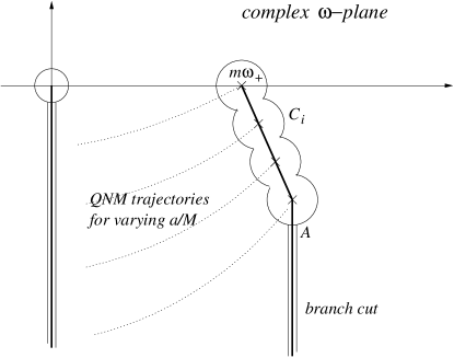
Figure 2: Schematic description of the QNM location (crosses) and placement of the required branch cuts (solid lines) in the case of an extreme Kerr black hole.

We now compute the mode-sum (62). The quantity $\alpha_{n}$ can be deduced from the derivative of the mode-condition (or equivalently, by taking the $a=M$ limit in (59) ). We get

$$\left.{df\over d\omega}\right|_{\omega=\omega_{n}}\approx-8imM\delta_{n}\exp\left[\left(i-{1\over 2\delta_{n}}\right)(\chi-2n\pi)+i(2i\delta_{n}-1)\zeta\right]\ .$$ (67)

Given this, we find that

$${A^{\rm out}\over\alpha_{n}}\approx(-1)^{1/2+im+i\delta_{n}}(im)^{2im}\frac{\Gamma(1/2-im-i\delta_{n})}{\Gamma(1/2+im-i\delta_{n})}qe^{i\chi}\left[e^{2\pi\delta_{n}}-\frac{\Gamma(1/2-im+i\delta_{n})\Gamma(1/2+im-i\delta_{n})}{\Gamma(1/2-im-i\delta_{n})\Gamma(1/2+im+i\delta_{n})}\right]\left[{df\over d\omega}\right]_{\omega=\omega_{n}}^{-1}\ .$$ (68)

Hence, we have shown that

$${A^{\rm out}\over\alpha_{n}}\sim e^{-n\pi/\delta_{n}}$$ (69)

i.e. each long-lived QNM is excited to an exponentially small amplitude. The total QNM response, $S_{\rm M}$, can now be approximated by

$$S_{\rm M}\sim\sum_{n=N}^{+\infty}\frac{A^{\rm out}}{\alpha_{n}}e^{-i\omega_{n}(t-r_{\ast}-r_{\ast}^{\prime})}\ .$$ (70)

Using (68) and (54), we see that,

$$S_{\rm M}\sim\sum_{n=N}^{+\infty}\exp\left[-(1-2i\delta){n\pi\over\delta}-\beta e^{-n\pi/\delta}\right]\ ,$$ (71)

where $\beta=iu\exp(\theta/2\delta-i\varphi)/4mM$, and we have introduced the retarded time $u=t-r_{\ast}-r_{\ast}^{\prime}$. This can be written as

$$S_{\rm M}\sim\sum_{n=0}^{+\infty}\exp\left[-(1-2i\delta){n\pi\over\delta}-\tilde{\beta}e^{-n\pi/\delta}\right]\ ,$$ (72)

with $\tilde{\beta}=\beta e^{N\pi/\delta}$. Since the main contribution to the sum is coming from the large values of $n$, we can approximate the sum by an integral,

$$S_{\rm M}\sim{\delta\over\pi}\int_{0}^{\infty}\exp\left[-\alpha x-\tilde{\beta}e^{-x}\right]dx$$ (73)

where $\alpha=1-2i\delta$. Expanding the expression in the bracket as a Taylor series and integrating we get

$$S_{\rm M}\sim{\delta\over\pi}\sum_{k=0}^{\infty}{(-1)^{k}\tilde{\beta}^{k}\over k!(k+\alpha)}={\delta\over\pi}\tilde{\beta}^{-\alpha}\gamma(\alpha,\tilde{\beta})\ ,$$ (74)

after identifying the series representation of the incomplete gamma function stegun . Since $\gamma(\alpha,\tilde{\beta})\to\Gamma(\alpha)$ as $\tilde{\beta}\to\infty$ we can deduce that

$$S_{\rm M}\sim{e^{-im\omega_{+}t}\over t}\quad\mbox{ as }t\to\infty\ .$$ (75)

Since this decays slower than (66) we can neglect the contribution from the extreme Kerr branch cut.

Next, we turn to the $l>m$ terms in (38). In view of the absence of any poles in the vicinity of $\omega=m\omega_{+}$, we simply place the branch cut parallel to the imaginary axis. The only multivalued quantity at $\omega=m\omega_{+}$ in the integrand of (38) is the ratio $A^{\rm out}/A^{\rm in}$ (see Appendix A). A standard branch cut calculation then yields

$$\Phi_{m}(r,\theta,t) = \frac{1}{4\pi M}\int_{-\infty}^{+\infty}dr_{\ast}^{\prime}e^{-imu/2M}\int_{0}^{-i\infty}d\tau e^{-i\tau/M}S_{lm}(\theta,a\tau/M+am/2M){\cal J}_{lm}(r_{\ast}^{\prime},\tau/M+m/2M)$$ (76)

$$\times\left[\frac{A^{\rm out}}{A^{\rm in}}(\tau e^{2\pi i}/M+m/2M)-\frac{A^{\rm out}}{A^{\rm in}}(\tau/M+m/2M)\right]$$

We can split the frequency integral into two parts (for brevity we omit the integrands):

$$\int_{0}^{-i\infty}d\tau\left\{...\right\}=\int_{0}^{-i\epsilon}d\tau\left\{...\right\}+\int_{-i\epsilon}^{-i\infty}d\tau\left\{...\right\}$$ (77)

The constant $\epsilon$ is chosen in order to allow us to use the $a=M$, $\omega\approx m\omega_{+}$ approximation

$$\frac{A^{\rm out}}{A^{\rm in}}(\omega,a=M) = (-1)^{1/2+2i\omega M+i\delta}(2i\omega M)^{4i\omega M}\frac{\Gamma(1/2-2i\omega M-i\delta)}{\Gamma(1/2+2i\omega M-i\delta)}$$ (78)

$$\times \left[\frac{\Gamma(2i\delta)\Gamma(1+2i\delta)\Gamma(1/2+2i\omega M-i\delta)\Gamma(1/2-2i\omega M-i\delta)}{\Gamma(-2i\delta)\Gamma(1-2i\delta)\Gamma(1/2-2i\omega M+i\delta)\Gamma(1/2+2i\omega M+i\delta)}+(8\omega M\tau)^{2i\delta}\right]$$

$$\times \left[{\Gamma(2i\delta)\over\Gamma(-2i\delta)}{\Gamma(1+2i\delta)\over\Gamma(1-2i\delta)}\left({\Gamma(1/2-2i\omega M-i\delta)\over\Gamma(1/2-2i\omega M+i\delta)}\right)^{2}+(-8\omega M\tau)^{2i\delta}\right]^{-1}$$

The key point here is that for $l\neq m$ the quantity $\delta$ is almost purely imaginary near $m\omega_{+}$, with positive imaginary part. We then have for $\tau\to 0$;

$$\tau^{2i\delta}\to+\infty$$ (79)

Hence, the expression inside the bracket in the first integral of the right-hand side of (77), will be vanishingly small and therefore the contribution from the part of the branch cut close to $m\omega_{+}$ is negligible for $l\neq m$. The second integral in (77) can be evaluated using arguments similar to the ones involved in the derivation of (66). We end up with an exponentially decaying field that can be neglected compared to (75).

Finally, we have to consider the contribution from the remaining QNMs. But because all these modes are “short-lived” their contribution is important only during the early phase of QNM ringing, cf. the Schwarzschild results na .

The main conclusion of this Section is that even though the contribution of each long lived QNM to the emerging field is exponentially small, the total mode contribution cannot be neglected. When summed, the slowly damped QNMs of an extreme Kerr black hole give rise to an oscillating signal whose magnitude falls off with time as a power-law. This result is particularly interesting since the decay of this signal is considerably slower than the standard power-law tail in the Kerr case hod ; barack1 ; barack2 . It is worth mentioning that oscillating power-laws are known to arise in standard scattering theory whenever the Green’s function has multiple poles newton . In our case, one could argue that it is the exponentially small “spacing” between neighbouring poles (see expression (54)) that causes the $1/t$ power-law.

It is also worth pointing out that the prediction (69) for the excitation of each individual long-lived QNM agrees with the intuitive arguments we made in the Introduction. For example, we see that the leading QNM is not excited for $a=M$ (as it corresponds to the limit $n\to\infty$ in (69)). This is in agreement with, and generalises, the $l=m\gg 1$ result (which is valid only for the fundamental mode) obtained in ferrari using the eikonal approximation.

IV Numerical results

IV.1 Time evolutions

In the previous Section we used analytic approximations to analyze the long-lived QNMs of a near extreme Kerr black hole. We obtained results that agree with our anticipations that these modes would not individually be excited to a significant level. But our calculation also provided surprises, the most important being that the large number of slowly damped QNMs combine to give a significant signal the amplitude of which falls of as $1/t$ at late times. However, in view of the many approximations involved in the derivation of (75) considerable caution is warranted, and a confirmation of the analytic prediction is desirable. One way to obtain support for the results would be to perform time-evolutions of the Teukolsky equation from given initial data. In other words, the recent effort to develop a framework for doing perturbative time-evolutions for Kerr black holes tcode1 ; tcode2 ; tcode3 ; tcode4 provides the means for testing our analytical predictions.

We have performed a set of evolutions (for various values of $m$) using the same scalar field code that was used to study superradiance in a dynamical context tcode4 . As initial data we have chosen a generic Gaussian pulse originally located far away from the black hole. The evolution of this pulse, as it travels towards the black hole and excites the QNM ringing is then studied. The numerical results we obtain support the following conclusions: i) In the case of extreme Kerr black holes ($a=M$) we verify the predicted oscillating $1/t$ behaviour for all $m\neq 0$, cf. Figure 3. ii) For $a<M$ we recover the anticipated exponential fall-off at late times, cf. tcode2 . Still, the emerging signal differs considerably from a single QNM oscillation at intermediate times for near extreme black holes. This agrees well with the analytical results from the previous Section: For near extreme black holes a large number of long-lived QNMs are excited to roughly the same level, and for a considerable time window the resulting signal is a superposition of many slowly decaying exponentials (each with a very small amplitude). As we depart further from $a=M$ we retain the standard result: The signal is completely dominated by the slowest damped QNM. iii) For axisymmetric perturbations ($m=0$) the numerical evolution recovers the standard power-law tail. For our particular choice of initial data (that contains the $l=0$ multipole) the tail falls off as $t^{-3}$. This agrees with the predictions of, for example, Ori and Barack barack1 ; barack2 .

Figure 3: A numerical evolution showing the late-time behaviour of a scalar field in the geometry of a rapidly rotating Kerr black hole. We show (on a logarithmic scale) the field as viewed by an observer situated well away from the black hole for $a=M$. At late times the field falls off according to an oscillating power-law with the amplitude decaying as $1/t$. The data corresponds to a narrow Gaussian (initially centered at $r_{\ast}=50M$) that hits the black hole, and is observed at $r_{\ast}=10M$

Although our numerical simulations generally support the analytic results, there is still room for some caution. It is very difficult to investigate the late-time behaviour of a perturbed Kerr black hole using the Teukolsky code. After all, we would like to be able to distinguish a slowly damped exponential from an oscillating power-law at very late times. Given our current numerical code we cannot obtained absolute proof of our analytic results. Detailed convergence tests show that the code has the expected properties, but also unveil that it is difficult to reliably determine the late time oscillating tail predicted by our analytical work. While the overall amplitude envelope can be determined for many hundred dynamical timescales as the resolution is increased, the signal typically goes out of phase on a shorter timescale. This means that, even though the numerical results provide support for our theoretical predictions, one would have to build an evolution code that could be trusted at very late times, eg. based on a double-null evolution, in order to obtain definite results.

Figure 4: We compare the late-time QNM oscillations in a typical scalar field evolution (initial data and observer location are the same as in Figure 3) for $m=2$ and $a=0.99M$ to the damping rates of the two slowest damped QNMs (indicated by dashed lines). From this figure it is clear that the late-time behaviour is not well represented by either of these modes individually.

IV.2 Reconstructing the long-lived QNM signal

In addition to investigating the late-time field through direct numerical evolutions, we can reconstruct it from our analytical results. Using expressions (55) - (59) it is a straightforward task to calculate the long-lived QNM signal provided that we have already acquired the corresponding mode-frequencies. In this way one can expect to obtain a fairly accurate description of the full signal for sufficiently late times (i.e. after some e-folding times of the dominant short-lived QNM: typically the slowest damped $m=-l$ mode), spanning a time window of several hundred dynamical timescales. Eventually one would expect this signal (after all, it decays exponentially) to give way to the standard power-law tail. However, as is clear from all our illustrations this will not happen until at very very late times.

In Table 1 we present a small subset of our numerical data for long-lived QNMs frequencies and the corresponding excitation coefficents for near extreme black holes. As anticipated, these amplitudes vanish as $a\to M$. Moreover, as already pointed out, the higher overtones are excited to a level comparable to the leading mode. In Figure 5 we illustrate the typical field as constructed from the long-lived QNMs. For this particular calculation, we have chosen, as initial data, a Gaussian pulse with angular dependence $\sim Y_{22}(\theta,\phi)$. It follows then from (55), that only the $l=m=2$ field component will be important at late times. The result in Figure 5 should be compared to the fully numerical evolution data in Figures 3-4.

Figure 5: The signal (shown on a logarithmic scale) from the long-lived QNMs (the first ten modes are included here), for an $a=0.9999M$ Kerr black hole. The required mode-data is given in Table 1. The observer is located at $r_{\ast}=100M,\theta=\pi/2$ and a narrow Gaussian pulse (centered at $r_{\ast}=50M$) was used as initial data. The dashed line represents the damping rate of the slowest decaying QNM. It is clear that for several hundreds of black hole’s dynamical times, the slowest damped mode is not dominant. This is in contrast to the results for slowly rotating black holes.

V A physical interpretation: The superradiance resonance cavity

Our analytical results, supported by the outcome of numerical evolutions, give rise to an intriguing picture. It would seem as if the extremely long-lived QNMs will, even though they are hardly excited at all individually, dominate the signal from a very rapidly spinning black hole. The emergence of this late-time signal, to which many QNMs contribute would be a new phenomenon in black-hole physics. Given that both the standard QNMs and the power-law tail have simple intuitive explanations it may be worthwhile trying to understand the extreme Kerr case in a similar way. From the evidence provided by our numerical evolutions, see Figure 8, we propose the following “explanation”. Consider the fate of an essentially monochromatic wave that falls onto the black hole, cf. Figure 6 for a schematic description. Provided that the frequency is in the interval $0<\omega<m\omega_{+}$ the wave will be superradiant: scattering of these waves in the black hole’s ergosphere results in their amplification by extraction of the black hole’s rotational energy. In effect, this means that a distant observer will see waves “emerging from the horizon”, cf. (32), even though a local observer sees the waves crossing the event horizon (at $r_{+}$) teuk2 . In addition to this, one can establish that the effective potential has a peak outside the black hole (which is not immediately obvious since the “potential” $Q$ is frequency dependent in the Kerr case) for a range of frequencies including the superradiant interval. Indeed, we can find the following approximate expression for the potential near the horizon (valid for $a=M$ only)

$$Q(r,\omega)=(\omega-m\omega_{+})^{2}-2(\omega-m\omega_{+})\frac{m}{r_{\ast}}+{\cal O}\left(\frac{\ln(r_{\ast}/M)}{r_{\ast}^{2}}\right)$$ (80)

This shows that, for $\omega\approx m\omega_{+}$, there will be a peak (corresponding to a minimum of $Q$) just outside the horizon. This can be verified by graphing the exact potential (29), cf. Figure 7.

Figure 6: Schematic explanation of the new phenomenon seen in the numerical evolutions of Kerr perturbations. The left panel illustrates the standard scenario: An infalling pulse excites the QNMs that then propagate to infinity and the horizon. At late times, backscattering due to the curvature in the far-zone dominates and leads to the familiar power-law tail behaviour. Right panel: For frequencies that i) lie in the superradiant regime, and ii) experience a “potential peak” in the region $[r_{+},\infty]$ there will be a superradiance resonance cavity outside the black hole. At late times, the waves leaking out of this cavity to infinity dominate the signal.

The combination of the causal boundary condition at the horizon effectively corresponding to waves “coming out of the black hole” (according to a distant observer) and the presence of a potential peak leads to waves potentially being trapped in the region close to the horizon. In effect, there is a “superradiance resonance cavity” outside the black hole. Again according to a distant observer, waves can only escape from this cavity by leakage through the potential barrier to infinity. Since the superradiant amplification is strongest for frequencies close to $m\omega_{+}$, waves in the cavity experience a kind of parametric amplification and at very late times the dominant oscillation frequency ought to be $m\omega_{+}$. This is exactly what we have deduced from our analytic and numerical calculations. In Figure 8 we present a series of snapshots of the evolution of a scalar field around an extreme Kerr black hole. In this series of pictures one can see how “trapped” oscillations develop in the vicinity of the black hole’s horizon. After an initial drop in amplitude (roughly at the timescale of the e-folding time of the rapidly damped “Schwarzschild-like” QNMs) these oscillations decay very slowly. These snapshots indicate the presence of a standing wave in the region just outside the horizon. In the extreme black hole case leakage from the superradiance cavity leads to the observed $1/t$ decay. In the near extreme case, the existence of the cavity provides an intuitive explanation for the extremely slow damping of corotating QNMs with frequencies close to $m\omega_{+}$. In a way, the superradiance cavity we have described here can be viewed as the black hole analogue of the potential “well” present in the gravitational field of ultracompact stars chandra2 which also leads to the existence of a long-lived family of $w$-modes ultra .

Figure 7: Graph of the $l=m=2$ effective radial potential $Q(r_{\ast},\omega)$ as a function of $r_{\ast}$, for $\omega=0.9m\omega_{+}$ (dashed curve), $m\omega_{+}$ (solid curve) , $1.1m\omega_{+}$ (dotted curve). The black hole spin is $a=0.999M$. Note the appearance of a potential barrier ($Q<0$) as soon as we enter the superradiant frequency regime $\omega<m\omega_{+}$.

Figure 8: A series of snapshots of a typical numerical evolution of a rapidly spinning black hole. We show the scalar field a function of both $r_{\ast}$ and $\theta$ at various times (as indicated in the upper right hand corner of each image). The images illustrate how “trapped” oscillations develop in the vicinity of the black hole’s horizon. After an initial drop in amplitude, cf. the first four images, (roughly at the timescale of the e-folding time of the rapidly damped “Schwarzschild-like” QNMs) these oscillations decay very slowly. These last four snapshots indicate the presence of a very slowly damped standing wave in the region just outside the horizon.

VI Concluding Discussion

We have presented the results of an investigation into the late-time behaviour of a perturbed Kerr black hole. An analytic calculation for scalar fields in the geometry of an extreme Kerr black hole provided two important results. The first concerns the level of excitation of the QNMs that become very slowly damped as $a\to M$. We find that these modes are much more difficult to excite than their rapidly damped Schwarzschild counterparts. This means that (individually) these modes may not be easy to detect with the new generation of gravitational-wave detectors. However, there may still be a detectable, slowly damped, QNM signal owing to the fact that a large number of virtually undamped QNMs exist for each value of $m\neq 0$. We find that these modes combine in such a way that the field oscillates with an amplitude that decays as $1/t$ at late times. This decay is considerably slower than the standard power-law tail. We have used numerical time-evolutions of the Teukolsky equation to verify this analytic prediction for extreme black holes.

After extending our study to near extreme black holes we find that, even though the QNM signal decays exponentially in the familiar way, there is still a considerable time interval where a large number of small-amplitude slowly-damped QNMs are present in the signal. This means that the signal from a rapidly spinning black hole would not be well represented by a single QNM approximation. Only at very late times do the leading mode become dominant and eventually it should give way to the power-law tail predicted in previous work barack1 ; barack2 ; hod .

Whether our results are astrophysically relevant or not is in many ways still an open question. In particular, the excitation of the long-lived QNMs by more realistic initial data (representing, for example, the close-limit approximation of merging Kerr black holes) must be studied. One should obviously also try to understand whether one would expect to find almost extreme black holes in Nature (recall that Thorne kip has shown that accretion cannot spin a black hole up beyond $a=0.998M$). It seems quite reasonable, however, to expect that the effects we have observed will play a role at intermediate times for rapidly rotating non-extreme black holes. If our predictions are correct one must investigate in detail to what extent the late-time signals from a rapidly rotating black-hole are detectable even though they contain a large number of QNMs (each with a small amplitude). In particular, it is crucial to determine whether one can hope to infer the black-hole parameters from a signal that contains such a superposition of QNMs (perhaps using techniques similar to those introduced in nollert ). It is also interesting to ask whether there exists a critical value of the rotation parameter $a$ above which the new effect we have observed becomes relevant (recall that our approximate modes are only relevant for $a\approx M$). More detailed numerical work is needed to answer this question. Finally, we note that the observed phenomenon can be intuitively explained in terms of a “superradiance resonance cavity” outside the black hole, in which waves of certain frequencies are effectively trapped. As the waves slowly leak out from this cavity, they give rise the “long-lived” QNM signal observed at infinity. In conclusion, it is interesting to note that, even though black-hole perturbations is a very well researched field, it can still provide interesting and surprising results.

Appendix A Approximate solutions of the Teukolsky equation for near extreme rotation

In this Appendix we reproduce the solution of the Teukolsky equation for $a\approx M$, $\omega\approx m\omega_{+}$, as given by Teukolsky and Press teuk2 . Throughout this paper we have (as far as possible) used the notation of their Appendix A1. The equation to be solved is not the “usual” Teukolsky equation, but the one that follows if we consider the problem in “ingoing Kerr” coordinates. These are related to the Boyer-Lindquist coordinates by

$$v = t+\int{r^{2}+a^{2}\over\Delta}dr\ ,$$ (81)

$$\tilde{\varphi} = \varphi+\int{a\over\Delta}dr\ .$$ (82)

In these coordinates the separation of variables follows from (note that the radial functions here differ from the one used in Section IIA by the factor $(r^{2}+a^{2})^{-1/2}$)

$$\Phi_{lm}=\int\tilde{R}_{lm}(\omega,r)S_{lm}(\theta,a\omega)e^{im\tilde{\varphi}-i\omega v}d\omega\ .$$ (84)

Comparing this expression to the standard Boyer-Lindquist decomposition

$$\Phi_{lm}=\int R_{lm}(\omega,r)S_{lm}(\theta,a\omega)e^{im\varphi-i\omega t}d\omega\ ,$$ (85)

we can immediately relate the radial wavefunctions via

$$R_{lm}(\omega,r)=\tilde{R}_{lm}(\omega,r)\exp\left[-i\int{K\over\Delta}dr\right]\ .$$ (86)

Since

$$\int{K\over\Delta}dr\sim\left\{\begin{array}[]{ll}\omega r_{\ast}\ ,\quad\mbox{ as }r_{\ast}\to+\infty\ ,\\ kr_{\ast}\ ,\quad\mbox{ as }r_{\ast}\to-\infty\ .\end{array}\right.\\$$ (87)

where we recall that $k=\omega-m\omega_{+}$. Hence, we see that the “physically acceptable” solution behaves as

$$\tilde{R}^{\rm in}\sim\left\{\begin{array}[]{ll}1\quad\quad\quad\mbox{as}\quad r\to r_{+}\ ,\\ Z^{\rm out}r^{-1}e^{2i\omega r_{\ast}}+Z^{\rm in}r^{-1}\quad\mbox{as }r\to+\infty\ .\end{array}\right.$$ (88)

In ingoing Kerr coordinates, the radial Teukolsky equation takes the form,

$$x(x+\sigma)\frac{d^{2}\tilde{R}_{lm}}{dx^{2}}-\{2i\hat{\omega}x^{2}+2x(2i\hat{\omega}-1)-\sigma+4i\tau\}\frac{d\tilde{R}_{lm}}{dx}-\{2i\hat{\omega}(x+1)+\lambda\}\tilde{R}_{lm}=0$$ (89)

The variables $x$ etcetera were defined by (42)-(46). The double limit $a\to M$, $\omega\to m\omega_{+}$ corresponds to $\sigma\to 0$, $~{}\tau\to 0$. Let us first consider this equation in the limit when $x>>\mbox{max }(\sigma,\tau)$, i.e., for large radii. Then (89) is well approximated by

$$x^{2}\frac{d^{2}\tilde{R}_{lm}}{dx^{2}}-\{2i\hat{\omega}x^{2}+2x(2i\hat{\omega}-1)\}\frac{d\tilde{R}_{lm}}{dx}-\{2i\hat{\omega}(x+1)+\lambda\}\tilde{R}_{lm}=0\ .$$ (90)

A solution to (90) that satisfies (88) can be written in terms of confluent hypergeometric functions stegun

$$\tilde{R}_{lm}=Ax^{-1/2+2i\hat{\omega}+i\delta}M(1/2+2i\hat{\omega}+i\delta,1+2i\delta,2i\hat{\omega}x)+B(\delta\rightarrow-\delta)$$ (91)

where $A$,$B$ are constants and the notation $(\delta\rightarrow-\delta)$ means “replace $\delta$ by $-\delta$ in the preceding term”. We next turn to the case when $x<<1$, i.e., try to find a solution that is valid close to the black hole’s horizon. The original equation simplifies (slightly) to

$$x(x+\sigma)\frac{d^{2}\tilde{R}_{lm}}{dx^{2}}-\{2x(2i\hat{\omega}-1)-\sigma+4i\tau)\}\frac{\tilde{R}_{lm}}{dx}-\{2i\hat{\omega}+\lambda\}\tilde{R}_{lm}=0\ .$$ (92)

This is the hypergeometric equation, and one solution can be written as

$$\tilde{R}_{lm}={}_{2}F_{1}(1/2-2i\hat{\omega}+i\delta,1/2-2i\hat{\omega}-i\delta,1-4i\tau/\sigma,-x/\sigma)\ .$$ (93)

It is straightforward to verify that ${}_{2}F_{1}\to 1$ as $x\to 0$, which means that this solution has the desired “purely ingoing wave” behaviour close to the event horizon. The solutions (91) and (93) can be matched in the overlap region, max($\sigma$,$\tau$) $\ll x\ll 1$. The $x\to 0$ limit of (91) yields,

$$\tilde{R}_{lm}\to Ax^{-1/2+2i\hat{\omega}+i\delta}+B(\delta\to-\delta)$$ (94)

Similarly, for $x\to\infty$, (93) becomes,

$$\tilde{R}_{lm}\to\frac{\Gamma(1-4i\tau/\sigma)\Gamma(2i\delta)\sigma^{1/2-2i\hat{\omega}-i\delta}}{\Gamma(1/2-2i\hat{\omega}+i\delta)\Gamma(1/2+2i\hat{\omega}+i\delta+4i\tau/\sigma)}x^{-1/2+2i\hat{\omega}+i\delta}+(\delta\to-\delta)$$ (95)

We can extract $A$ and $B$ by matching the solutions (94) and (95),

$$A = \frac{\Gamma(1-4i\tau/\sigma)\Gamma(2i\delta)\sigma^{1/2-2i\hat{\omega}-i\delta}}{\Gamma(1/2-2i\hat{\omega}+i\delta)\Gamma(1/2+2i\hat{\omega}+i\delta-4i\tau/\sigma)}$$ (96)

$$B = \frac{\Gamma(1-4i\tau/\sigma)\Gamma(-2i\delta)\sigma^{1/2-2i\hat{\omega}+i\delta}}{\Gamma(1/2-2i\hat{\omega}-i\delta)\Gamma(1/2+2i\hat{\omega}-i\delta-4i\tau/\sigma)}$$ (97)

On the other hand, approximating (91) for $x\to\infty$ we get for the amplitudes $Z^{\rm in}$,$Z^{\rm out}$,

$$Z^{\rm in} = r_{+}A\frac{\Gamma(1+2i\delta)}{\Gamma(1/2-2i\hat{\omega}+i\delta)}(-2i\hat{\omega})^{-1/2-2i\hat{\omega}-i\delta}+B(\delta\to-\delta)$$ (98)

$$Z^{\rm out} = r_{+}A\frac{\Gamma(1+2i\delta)}{\Gamma(1/2+2i\hat{\omega}+i\delta)}(2i\hat{\omega})^{-1/2+2i\hat{\omega}-i\delta}+B(\delta\to-\delta)$$ (99)

Using (86), it is easy to see that $A^{\rm in}=Z^{\rm in}$ and $A^{\rm out}=Z^{\rm out}$ where $A^{\rm out}$ and $A^{\rm in}$ are the asymptotic amplitudes in the standard Boyer-Lindquist decomposition. Explicitly we get

$$A^{\rm in}(\omega) = r_{+}(-2i\hat{\omega})^{-1/2-2i\hat{\omega}-i\delta}\sigma^{1/2-2i\hat{\omega}-i\delta}\frac{\Gamma(-2i\delta)\Gamma(1-2i\delta)\Gamma(1-4i\tau/\sigma)}{(\Gamma(1/2-2i\hat{\omega}-i\delta))^{2}\Gamma(1/2+2i\hat{\omega}+i\delta-4i\tau/\sigma)}$$ (100)

$$\times \left[{\Gamma(2i\delta)\over\Gamma(-2i\delta)}{\Gamma(1+2i\delta)\over\Gamma(1-2i\delta)}\left({\Gamma(1/2-2i\hat{\omega}-i\delta)\over\Gamma(1/2-2i\hat{\omega}+i\delta)}\right)^{2}+(-2i\hat{\omega}\sigma)^{2i\delta}{\Gamma(1/2+2i\hat{\omega}+i\delta-4i\tau/\sigma)\over\Gamma(1/2+2i\hat{\omega}-i\delta-4i\tau/\sigma)}\right]$$

$$A^{\rm out}(\omega) = r_{+}(2i\hat{\omega})^{-1/2+2i\hat{\omega}-i\delta}\sigma^{1/2-2i\hat{\omega}-i\delta}\frac{\Gamma(-2i\delta)\Gamma(1-2i\delta)}{\Gamma(1/2+2i\hat{\omega}-i\delta)\Gamma(1/2-2i\hat{\omega}-i\delta)}\frac{\Gamma(1-4i\tau/\sigma)}{\Gamma(1/2+2i\hat{\omega}+i\delta-4i\tau/\sigma)}$$ (101)

$$\times \left[\frac{\Gamma(2i\delta)\Gamma(1+2i\delta)\Gamma(1/2+2i\hat{\omega}-i\delta)\Gamma(1/2-2i\hat{\omega}-i\delta)}{\Gamma(-2i\delta)\Gamma(1-2i\delta)\Gamma(1/2-2i\hat{\omega}+i\delta)\Gamma(1/2+2i\hat{\omega}+i\delta)}+(2i\hat{\omega}\sigma)^{2i\delta}\frac{\Gamma(1/2+2i\hat{\omega}+i\delta-4i\tau/\sigma)}{\Gamma(1/2+2i\hat{\omega}-i\delta-4i\tau/\sigma)}\right]$$

and their ratio will be

$$\frac{A^{\rm out}}{A^{\rm in}} = (-1)^{1/2+2i\hat{\omega}+i\delta}(2i\hat{\omega})^{4i\hat{\omega}}\frac{\Gamma(1/2-2i\hat{\omega}-i\delta)}{\Gamma(1/2+2i\hat{\omega}-i\delta)}$$ (102)

$$\times \left[\frac{\Gamma(2i\delta)\Gamma(1+2i\delta)\Gamma(1/2+2i\hat{\omega}-i\delta)\Gamma(1/2-2i\hat{\omega}-i\delta)}{\Gamma(-2i\delta)\Gamma(1-2i\delta)\Gamma(1/2-2i\hat{\omega}+i\delta)\Gamma(1/2+2i\hat{\omega}+i\delta)}+(2i\hat{\omega}\sigma)^{2i\delta}\frac{\Gamma(1/2+2i\hat{\omega}+i\delta-4i\tau/\sigma)}{\Gamma(1/2+2i\hat{\omega}-i\delta-4i\tau/\sigma)}\right]$$

$$\times \left[{\Gamma(2i\delta)\over\Gamma(-2i\delta)}{\Gamma(1+2i\delta)\over\Gamma(1-2i\delta)}\left({\Gamma(1/2-2i\hat{\omega}-i\delta)\over\Gamma(1/2-2i\hat{\omega}+i\delta)}\right)^{2}+(-2i\hat{\omega}\sigma)^{2i\delta}{\Gamma(1/2+2i\hat{\omega}+i\delta-4i\tau/\sigma)\over\Gamma(1/2+2i\hat{\omega}-i\delta-4i\tau/\sigma)}\right]^{-1}$$

In the special case of an extreme Kerr black hole we have $\sigma=0$, and (102) then reduces to

$$\left.\frac{A^{\rm out}}{A^{\rm in}}\right|_{a=M} = (-1)^{1/2+2i\omega M+i\delta}(2i\omega M)^{4i\omega M}\frac{\Gamma(1/2-2i\omega M-i\delta)}{\Gamma(1/2+2i\omega M-i\delta)}$$ (103)

$$\times \left[\frac{\Gamma(2i\delta)\Gamma(1+2i\delta)\Gamma(1/2+2i\omega M-i\delta)\Gamma(1/2-2i\omega M-i\delta)}{\Gamma(-2i\delta)\Gamma(1-2i\delta)\Gamma(1/2-2i\omega M+i\delta)\Gamma(1/2+2i\omega M+i\delta)}+(8\omega M\tau)^{2i\delta}\right]$$

$$\times \left[{\Gamma(2i\delta)\over\Gamma(-2i\delta)}{\Gamma(1+2i\delta)\over\Gamma(1-2i\delta)}\left({\Gamma(1/2-2i\omega M-i\delta)\over\Gamma(1/2-2i\omega M+i\delta)}\right)^{2}+(-8\omega M\tau)^{2i\delta}\right]^{-1}$$

Note that this expression is multivalued at $\omega=m\omega_{+}$ due to the presence of the $\tau^{2i\delta}$ term (see Appendix B).

Appendix B Analytical properties of solutions of the Teukolsky equation

In this Appendix we study the analytical properties of the $u^{\rm in}$ function in the complex $\omega$-plane. A much more rigorous and detailed treatment has been provided by Hartle and Wilkins hw . However, as we will show here their conclusion that $u^{\rm in}$ has a branch point for $a<M$ is incorrect. Instead, we find that $u^{\rm in}$ has a series of (physically insignificant) poles. Only for the special case $a=M$ do these poles disappear, and $u^{in}$ has indeed a branch point.

To begin we write the radial Teukolsky equation (27) in a more compact form (in this Appendix we shall be considering perturbations of an arbitrary spin $s$ field)

$$\frac{d^{2}u}{dr_{\ast}^{2}}+Q(r_{\ast},\omega)u=0\ .$$ (104)

It is a well-known fact in scattering theory newton that certain analytical properties (with relevance for the late-time behaviour of the field) of the solutions to an equation of the form (104), can be found by studying the asymptotic behaviour of these solutions as $r_{\ast}\to\pm\infty$. Therefore, we consider (104) in the limit $r\to r_{+}$. For $a<M$ the potential has the asymptotic form,

$$Q(r_{\ast},\omega)\approx(\omega-m\omega_{+})^{2}-V_{\rm h}(\omega)+V_{\rm o}(\omega)e^{cr_{\ast}}\quad\mbox{as}\quad r_{\ast}\to-\infty\ ,$$ (105)

where

$$V_{\rm h}(\omega)=2is(\omega-m\omega_{+}){(r_{+}-M)\over 2Mr_{+}}+s^{2}{(r_{+}-M)^{2}\over(2Mr_{+})^{2}}\ ,$$ (106)

and $c=(r_{+}-r_{-})/2Mr_{+}$. The explicit form of the $V_{\rm o}(\omega)$ function will not be required in the following. Setting

$$\Omega=(\omega-m\omega_{+})-{is(r_{+}-M)\over 2Mr_{+}}\ ,$$ (107)

equation (104) becomes

$${d^{2}u\over dr^{2}_{*}}+\left[\Omega^{2}-V_{\rm o}e^{cr_{\ast}}\right]u=0\ ,$$ (108)

near the horizon. This equation can be solved by employing the standard Born approximation. However, it turns out that we can solve it exactly newton . By setting $y=e^{cr_{\ast}}$ we can rewrite the equation as

$$y^{2}\frac{d^{2}u}{dy^{2}}+y\frac{du}{dy}+\frac{1}{c^{2}}\left(\Omega^{2}-V_{\rm o}y\right)u=0$$ (109)

This is a Bessel-type equation and the solution $u^{\rm in}$ is

$$u^{\rm in}(r_{\ast},\omega)=\left(\frac{-iV_{\rm o}^{1/2}}{c}\right)^{2i\Omega/c}\Gamma(1-2i\Omega/c)J_{-2i\Omega/c}\left(\frac{-2iV_{\rm o}^{1/2}}{c}e^{cr_{\ast}/2}\right)$$ (110)

From the small argument approximation for the Bessel function (recall that $r_{\ast}\to-\infty$ as we approach the horizon), it is easy to see that this solution indeed satisfies the appropriate boundary behaviour at the horizon: $u^{\rm in}\to\Delta^{-s/2}e^{-ikr_{\ast}}$. The presence of the $\Gamma$ function signals the existence of simple poles at the points $1-2i\Omega/c=-n$ (where $n$ a non-negative integer) or, equivalently, at frequencies

$$\omega=m\omega_{+}+i(s-n-1)\frac{r_{+}-r_{-}}{4Mr_{+}}$$ (111)

If we had chosen to use the Born approximation, then at leading order, we would had picked up the first of these poles. The existence of these poles can be directly deduced by inspection of equation (93). These poles have, however, no physical significance. The black hole Green’s function does not inherit them since the factor $\Gamma(1-2i\Omega/c)$ will be cancelled by an identical factor in the Wronskian (in the $r_{\ast}\to+\infty$ form of $u^{\rm in}$ these poles are contained in the amplitudes $A^{\rm in}$, $A^{\rm out}$, see eqs. (96), (97) of Appendix A ). As a consequence, these are called “false” poles in quantum scattering theory newton .

Due to the appearance of the Bessel function of a noninteger power in (110), one would expect $u^{\rm in}$ to have branch points at those frequencies $\omega_{b}$ that solve $V_{\rm o}(\omega_{b})=0$. However, since $J_{\rm\nu}(ze^{2\pi i})=e^{2\pi\nu i}J_{\rm\nu}(z)$ stegun we are effectively left with a single-valued function. It is a quite general result in scattering theory that exponentially decaying potentials cannot lead to the existence of branch points newton .

We now turn to the $a=M$ case. Approximating the effective radial potential near the horizon for $a=M$ yields

$$Q(r,\omega)\approx(\omega-m\omega_{+})^{2}-2(\omega-m\omega_{+})\frac{(m-is)}{r_{\ast}}\quad\mbox{as}\quad r_{\ast}\to-\infty\ .$$ (112)

Near the horizon then, eqn. (104) effectively becomes

$$\frac{d^{2}u}{dr_{\ast}^{2}}+\left(\tilde{\Omega}^{2}+\frac{\beta}{r_{\ast}}\right)u=0$$ (113)

with $\tilde{\Omega}=\omega-m\omega_{+}$ and $\beta=-2(m-is)\tilde{\Omega}$. This equation can be easily transformed to a Whittaker equation stegun with two independent solutions $W_{\kappa,\mu}(2i\tilde{\Omega}r_{\ast}),W_{-\kappa,\mu}(-2i\tilde{\Omega}r_{\ast})$ where $\kappa=im+s,~{}\mu=\pm 1/2$. The Whittaker function $W_{\kappa,\mu}(z)$ is defined by,

$$W_{\kappa,\mu}(z) = z^{1/2+\mu}e^{-z/2}U(1/2+\mu-\kappa,1+2\mu,z)\ ,$$ (114)

Taking a large argument approximation for the confluent hypergeometric functions we deduce that $W_{\kappa,\mu}(2i\tilde{\Omega}r_{\ast})$ is the solution with the desired “ingoing wave” behaviour at the horizon. Clearly, $W_{\kappa,\mu}(z)$ is a multi-valued function with a branch point at $z=0$, which in the present case corresponds to $\omega=m\omega_{+}$. This is in agreement with the result of Hartle and Wilkins hw . In this case the branch point is inherited by the relevant Green’s function. More specifically, it is contained in the ratio $A^{\rm out}/A^{\rm in},~{}$ see equation (103).

Appendix C Gravitational perturbations

So far, we have mainly considered the model problem of a massless scalar field. We did this for reasons of simplicity. However, it turns out that our results are easily extended to the physically more interesting case of gravitational perturbations. In fact, the calculation proceeds very much along the same lines. This means that all conclusions reached in the main part of this paper remain valid also for the gravitational case.

In the Teukolsky formalism, gravitational perturbations are represented by the the scalar functions ${}_{s}\Psi$ with $s=\pm 2$ teuk1 . As before, we can separate the dependence on the $\varphi$ angle

$${}_{s}\Psi=\Delta^{-s/2}(r^{2}+a^{2})^{-1/2}\sum_{m=-\infty}^{+\infty}{}_{s}\psi_{m}(r,\theta,t)e^{im\varphi}$$ (116)

Further decomposition is possible in the Fourier domain

$${}_{s}\psi_{m}(r,\theta,t)={1\over 2\pi}\sum_{l={\rm max}(|m|,|s|)}^{\infty}\int_{-\infty+ic}^{+\infty+ic}{}_{s}R_{lm}(\omega,r){}_{s}S_{lm}(\theta,a\omega)e^{-i\omega t}d\omega\ .$$ (117)

where ${}_{s}R_{lm}$ solves (27) with the potential,

$$Q(r,\omega)={K^{2}-2is(r-M)K+(4i\omega rs-2am\omega-a^{2}\omega^{2}-E)\Delta\over(r^{2}+a^{2})^{2}}-{dG\over dr_{\ast}}-G^{2}$$ (118)

with $G=s(r-M)/(r^{2}+a^{2})+r\Delta/(r^{2}+a^{2})^{2}$. The solutions of the homogeneous equation (27) which are used for the construction of the Green’s function are now

$${}_{s}u^{\rm up}\sim\left\{\begin{array}[]{ll}{}_{s}D^{\rm out}\Delta^{s/2}e^{ikr_{\ast}}+{}_{s}D^{\rm in}\Delta^{-s/2}e^{-ikr_{\ast}}\quad\mbox{as }r\to r_{+}\ ,\\ r^{-s}e^{i\omega r_{\ast}}\quad\mbox{as }r\to+\infty\ ,\end{array}\right.$$ (119)

and

$${}_{s}u^{\rm in}\sim\left\{\begin{array}[]{ll}\Delta^{-s/2}e^{-ikr_{\ast}}\quad\mbox{as }r\to r_{+}\ ,\\ {}_{s}A^{\rm out}r^{-s}e^{i\omega r_{\ast}}+{}_{s}A^{\rm in}r^{s}e^{-i\omega r_{\ast}}\quad\mbox{as }r\to+\infty\ .\end{array}\right.$$ (120)

Repeating the same steps as in Section IIA, we end up with an expression similar to (38)

$${}_{s}\psi_{m}(r,\theta,t)\approx-\frac{1}{2\pi r^{s}}\sum_{l={\rm max}(|m|,|s|)}^{\infty}\int_{-\infty+ic}^{+\infty+ic}\frac{e^{-i\omega(t-r_{\ast})}}{2i\omega}{}_{s}S_{lm}^{a\omega}(\theta)\left[\frac{{}_{s}A^{\rm out}}{{}_{s}A^{\rm in}}{}_{s}{\cal I}_{lm}^{+}(\omega)+{}_{s}{\cal I}_{lm}^{-}(\omega)\right]$$ (121)

The analytical properties of the Green’s function are identical to the scalar case (recall that the analysis in Appendix B is valid for an arbitrary spin field). The long-lived QNMs are now solutions of detweiler

$$-\frac{\Gamma(2i\delta)\Gamma(1+2i\delta)\Gamma(1/2+s-2i\hat{\omega}-i\delta)\Gamma(1/2-s-2i\hat{\omega}-i\delta)}{\Gamma(-2i\delta)\Gamma(1-2i\delta)\Gamma(1/2+s-2i\hat{\omega}+i\delta)\Gamma(1/2-s-2i\hat{\omega}+i\delta)}=(-2i\hat{\omega}\sigma)^{2i\delta}{\Gamma(1/2+2i\hat{\omega}+i\delta-4i\tau/\sigma)\over\Gamma(1/2+2i\hat{\omega}-i\delta-4i\tau/\sigma)}\ .$$ (122)

This equation turns out to be invariant under the change $s\to-s$. It thus follows that the $s=\pm 2$ components share the same set of long-lived QNMs.

We need to find approximate ($a\approx M,\omega\approx m\omega_{+}$) expressions for the coefficients ${}_{s}A^{\rm in},{}_{s}A^{\rm out}$. Press and Teukolsky teuk2 give the relevant approximate radial wavefunctions in a Kerr-ingoing coordinates. We need to relate their solutions to the respective wavefunctions ${}_{s}u^{\rm in},{}_{s}u^{\rm up}$ in order to extract the asymptotic amplitudes ${}_{s}A^{\rm in}$ and ${}_{s}A^{\rm out}$. In the standard Boyer-Lindquist coordinates, a spin-$s$ field can be decomposed as

$${}_{s}\Psi={}_{s}{\cal R}_{lm}(r,\omega){}_{s}S_{lm}^{a\omega}(\theta)e^{im\varphi-i\omega t}\ .$$ (123)

Similarly, in Kerr-ingoing coordinates, we get

$${}_{s}\tilde{\Psi}={}_{s}\tilde{{\cal R}}_{lm}(r,\omega){}_{s}S_{lm}^{a\omega}(\theta)e^{im\tilde{\varphi}}e^{-i\omega\upsilon}\ .$$ (124)

These two representations are related by teuk2

$${}_{-s}\Psi=\left(\frac{\Delta}{2}\right)^{s}{}_{s}\tilde{\Psi}\ .$$ (125)

We adopt the following normalisation for the “in” radial wavefunctions, at $r\to\infty$ (hereafter, for brevity, we drop the $lm$ subscript)

$${}_{s}{\cal R}^{\rm in}\sim\left\{\begin{array}[]{ll}\Delta^{-s}e^{-ikr_{\ast}}\quad\mbox{as }r\to r_{+}\ ,\\ \quad{}_{s}B^{\rm in}r^{-1}e^{-i\omega r_{\ast}}+{}_{s}B^{\rm out}r^{-2s-1}e^{i\omega r_{\ast}}\quad\mbox{as }r\to+\infty\ .\end{array}\right.$$ (126)

$${}_{s}\tilde{{\cal R}}^{\rm in}\sim\left\{\begin{array}[]{ll}1\quad\mbox{as }r\to r_{+}\ ,\\ \quad{}_{s}Z^{\rm in}r^{-2s-1}+{}_{s}Z^{\rm out}r^{-1}e^{2i\omega r_{\ast}}\quad\mbox{as }r\to+\infty\ .\end{array}\right.$$ (127)

We are mainly interested in the $s=-2$ component, as it leads to the dominant contribution to the gravitational waves reaching infinity teuk1 . Inspection of (120) and (126) gives,

$$\frac{{}_{-2}A^{\rm in}}{{}_{-2}A^{\rm out}}=\frac{{}_{-2}B^{\rm in}}{{}_{-2}B^{\rm out}}$$ (128)

From (125) and (126) we obtain,

$${}_{-2}{\cal R}^{\rm in}=f\Delta^{2}{}_{2}\tilde{{\cal R}}^{\rm in}\exp\left[-i\int\frac{K}{\Delta}dr\right]$$ (129)

where $f$ some proportionality factor. Furthermore, it is possible to relate the two $s=-2$ fields, by means of the Starobinsky identity teuk2 :

$${}_{-2}{\cal R}_{lm}(r,\omega)=\frac{\Delta^{2}}{4|C|^{2}}J_{+}^{4}[\Delta^{2}{}_{2}{\cal R}_{lm}(r,\omega)]$$ (130)

where $J_{+}=d/dr+iK/\Delta$ and

$$|C|^{2}=(\lambda^{2}+4a\omega m-4a^{2}\omega^{2})[(\lambda-2)^{2}+36a\omega m-36a^{2}\omega^{2}]+(2\lambda-1)(96a^{2}\omega^{2}-48a\omega m)+144\omega^{2}(M^{2}-a^{2})$$ (131)

with $\lambda=E+a^{2}\omega^{2}-2a\omega m$. Combining (129) and (130) we get

$${}_{-2}{\cal R}=f\frac{\Delta^{2}}{4|C|^{2}}\frac{d^{4}}{dr^{4}}({}_{-2}\tilde{{\cal R}})e^{-i\int\frac{K}{\Delta}dr}$$ (132)

Eqns. (129) and (132) can be used to relate the coefficients (${}_{-2}A^{\rm in},{}_{-2}A^{\rm out}$) to (${}_{2}Z^{\rm in},{}_{2}Z^{\rm out}$) and (${}_{-2}Z^{\rm in},{}_{-2}Z^{\rm out}$), respectively. The first of these connecting formulas simply yields ${}_{-2}A^{\rm in}/{}_{-2}A^{\rm out}={}_{2}Z^{\rm in}/{}_{2}Z^{\rm out}$. The QNM frequencies therefore satisfy

$$\left.\frac{{}_{-2}A^{\rm in}}{{}_{-2}A^{\rm out}}\right|_{\omega=\omega_{n}}=\left.\frac{{}_{2}Z^{\rm in}}{{}_{2}Z^{\rm out}}\right|_{\omega=\omega_{n}}=0$$ (133)

This equation yields (122) for $s=2$, which is, as pointed out, invariant under the operation $s\to-s$. It is easy to verify that the long-lived gravitational QNMs are given by an expression similar to (54). We have,

$$\frac{{}_{-2}A^{\rm out}}{{}_{-2}A^{\rm in}}(\omega) = r_{+}^{-4}(2i\hat{\omega})^{4+4i\hat{\omega}}\frac{\Gamma(-3/2-2i\hat{\omega}-\delta)}{\Gamma(5/2+2i\hat{\omega}-i\delta)}$$ (134)

$$\times \left[{\Gamma(2i\delta)\over\Gamma(-2i\delta)}{\Gamma(1+2i\delta)\over\Gamma(1-2i\delta)}{\Gamma(5/2-2i\hat{\omega}-i\delta)\Gamma(-3/2-2i\hat{\omega}-i\delta)\over\Gamma(5/2-2i\hat{\omega}+i\delta)\Gamma(-3/2-2i\hat{\omega}+i\delta)}+(-2i\hat{\omega}\sigma)^{2i\delta}{\Gamma(1/2+2i\hat{\omega}+i\delta-4i\tau/\sigma)\over\Gamma(1/2+2i\hat{\omega}-i\delta-4i\tau/\sigma)}\right]^{-1}$$

$$\times \left[\frac{\Gamma(2i\delta)\Gamma(1+2i\delta)\Gamma(5/2+2i\hat{\omega}-i\delta)\Gamma(5/2-2i\hat{\omega}-i\delta)}{\Gamma(-2i\delta)\Gamma(1-2i\delta)\Gamma(5/2-2i\hat{\omega}+i\delta)\Gamma(5/2+2i\hat{\omega}+i\delta)}+(2i\hat{\omega}\sigma)^{2i\delta}\frac{\Gamma(1/2+2i\hat{\omega}+i\delta-4i\tau/\sigma)}{\Gamma(1/2+2i\hat{\omega}-i\delta-4i\tau/\sigma)}\right]$$

It follows that the analysis presented in Section IIE can be used also in the gravitational case, yielding results indentical to the scalar ones.

We note that the gravitational perturbation problem can alternatively be approached exclusively via the $s=-2$ fields, see equation (132). This choice was made by Sasaki and Nakamura sasaki in their study of the late-time response of an extreme Kerr hole perturbed by an orbiting test particle. Their results do not agree with ours in that they find that the late-time signal decays as $\sim 1/t^{1/2}$. Such a power-law would lead to an (unphysical) divergent flux integral sasaki . We believe that the calculation of Sasaki and Nakamura contains an error in the relation between the relevant asymptotic amplitudes. According to their result, the ratio of the asymptotic amplitudes ${}_{-2}B^{\rm in}/{}_{-2}B^{\rm out}$ introduces additional powers of $\tau$ in the integrand of (121) which then leads to the different power-law behaviour. We have perfomed the calculation (using equations (132), (91)) and found

$$\frac{{}_{-2}B^{\rm in}}{{}_{-2}B^{\rm out}}=r_{+}^{8}D(\omega)\frac{{}_{-2}Z^{\rm in}}{{}_{-2}Z^{\rm out}}$$ (135)

with

$$D(\omega)=(2i\hat{\omega})^{-4}\left((2\hat{\omega}+\delta)^{4}+\frac{5}{2}(2\hat{\omega}+\delta)^{2}+\frac{9}{16}\right)\left((2\hat{\omega}-\delta)^{4}+\frac{5}{2}(2\hat{\omega}-\delta)^{2}+\frac{9}{16}\right)$$ (136)

which differs crucially from the result of Sasaki and Nakamura. However, given that several derivatives of the asymptotic solutions are required to derive this result, and that significant cancellations occur, it would be very easy to make a mistake in this calculation.

$n$	Re $\omega_{n}M$	Im $\omega_{n}M$	Re $(MA^{\rm out}/\alpha_{n})$	Im $(MA^{\rm out}/\alpha_{n})$
0	0.99324	-0.00341	0.00216	-0.00369
1	0.99322	-0.01020	-0.00691	-0.00928
2	0.99321	-0.01699	-0.02167	0.01501
3	0.99320	-0.02385	-0.02167	0.01501
4	0.99317	-0.03067	-0.01288	0.03089
5	0.99313	-0.03749	0.00398	0.04030
6	0.99308	-0.04432	0.02439	0.040882
7	0.99303	-0.05115	0.04427	0.03253
8	0.99298	-0.05798	0.06043	0.01643
9	0.99291	-0.06482	0.07055	-0.00550

Table 1: Frequencies and excitation coefficients for the first ten $l=m=2$ QNMs, for an $a=0.9999M$ Kerr black hole. These results illustrate the fact that many QNMs are excited to a comparable amplitude (cf. the excitation coefficients listed in the last two columns).

References

- (1) C.V. Vishveshwara, Nature 227 936 (1969)
- (2) R.H. Price, Phys. Rev. D 5 2419 (1972); ibid 5 2439 (1972)
- (3) Chapter 4 in Black-hole physics by V.P. Frolov and I.D. Novikov (Kluwer, Dordrecht 1998)
- (4) C. Gundlach, R.H. Price and J. Pullin Phys. Rev. D 49 883 (1994)
- (5) N. Andersson and K.D. Kokkotas, Phys. Rev. Lett. 77 4134 (1996)
- (6) E.W. Leaver, Phys. Rev. D 34 384 (1986)
- (7) N. Andersson, Phys. Rev. D 55 468 (1997)
- (8) E.W. Leaver, Proc. R. Soc. Lond. A 402, 285 (1985)
- (9) H. Onozawa, Phys. Rev. D 55 3593 (1997)
- (10) W. Krivan, P. Laguna and P. Papadopoulos, Phys. Rev D 54 4728 (1996)
- (11) W. Krivan, P. Laguna, P. Papadopoulos and N. Andersson, Phys. Rev. D 56 3395 (1997)
- (12) N. Andersson, P. Laguna and P. Papadopoulos, Phys. Rev. D 58 087503 (1998)
- (13) W. Krivan and R.H. Price, Phys. Rev. D 58 104003 (1998); Phys. Rev. Lett. 82 1358 (1999)
- (14) S. Hod, Phys. Rev. D 58 104022 (1998); ibid 60 104053 (1999); ibid 61 024033 (2000); ibid 61 064018 (2000)
- (15) L. Barack and A. Ori, Phys. Rev. Lett. 82 4388 (1999)
- (16) L. Barack, Phys Rev D 61 024026 (2000)
- (17) A. Ptak and R. Griffiths, Ap. J. Lett. 517 85 (1999)
- (18) E.J.M. Colbert and R.F. Mushotzky, Ap. J. 519 89 (1999)
- (19) S. Detweiler, Astrophys. J. 225 687 (1978)
- (20) F. Echeverria, Phys. Rev. D 40 3194 (1989)
- (21) L.S. Finn, Phys. Rev. D 46 5236 (1992)
- (22) E.E. Flanagan and S. A. Hughes, Phys. Rev. D 57 4535 (1998)
- (23) H.P. Nollert and R.H. Price, J. Math. Phys. 40 980 (1999)
- (24) V. Ferrari and B. Mashhoon, Phys. Rev. D 30 295 (1994)
- (25) N. Andersson and K. Glampedakis, Phys. Rev. Lett 84 4537 (2000)
- (26) N. Andersson and K. Glampedakis, A quick and dirty method for calculating black hole resonances, in preparation (2001)
- (27) S.A. Teukolsky and W.H. Press, Astrophys. J. 193 443 (1974)
- (28) R.H. Price and J. Pullin, Phys. Rev. Lett. 72 3297 (1994)
- (29) J. Baker, B. Bruegmann, M. Campanelli and C. O. Lousto, Class. Quant. Grav. 17 L149 (2000)
- (30) M. Campanelli and C.O. Lousto, Phys. Rev. D 59 124022 (1999)
- (31) S. Chandrasekhar, The Mathematical Theory of Black Holes (Oxford University Press, New York, 1983)
- (32) S.A. Teukolsky Phys. Rev. Lett. 29 1114 (1972)
- (33) J.B. Hartle and D.C. Wilkins, Commun. Math. Phys. 38 47 (1974)
- (34) E.S.C. Ching, P.T. Leung, W.M. Suen and K. Young Phys. Rev. D 52, 2118 (1995)
- (35) M. Sasaki and T. Nakamura, Gen. Rel. Grav. 22 1351 (1990)
- (36) M. Abramowitz and I.A. Stegun, Handbook of Mathematical Functions (Dover Publications Inc., New York, 1985)
- (37) R.G. Newton, Scattering theory of waves and particles (McGraw-Hill, 1966)
- (38) S. Chandrasekhar and V. Ferrari, Proc. R. Soc. Lond. A 434, 449 (1991)
- (39) K.D. Kokkotas, Mon. Not. R. Astron. Soc. 268, 1015 (1994)
- (40) K.S. Thorne, Astrophys. J. 191 507 (1974)