Exact relativistic treatment of stationary counter-rotating dust disks II
Axis, Disk and Limiting Cases

Abstract

This is the second in a series of papers on the construction of explicit solutions to the stationary axisymmetric Einstein equations which can be interpreted as counter-rotating disks of dust. We discuss the class of solutions to the Einstein equations for disks with constant angular velocity and constant relative density which was constructed in the first part. The metric for these spacetimes is given in terms of theta functions on a Riemann surface of genus 2. We discuss the metric functions at the axis of symmetry and the disk. Interesting limiting cases are the Newtonian limit, the static limit, and the ultra-relativistic limit of the solution in which the central redshift diverges.

PACS numbers: O4.20.Jb, 02.10.Rn, 02.30.Jr

1 Introduction

The stationary axisymmetric Einstein equations are of great physical importance since their solutions can describe the gravitational field of stars and galaxies in thermodynamical equilibrium. In this case the matter can be approximated as an ideal fluid, but the field equations in the matter region do not seem to be integrable. The vacuum equations are however equivalent to the Ernst equation [1] which is completely integrable [2, 3, 4]. If one considers two-dimensional matter distributions as disks which are discussed as models for the matter in galaxies or in accretion disks around black-holes, the matter leads to a boundary value problem for the vacuum equations. A solution to this boundary value problem leads to global spacetimes with matter distributions which can be physically interpreted.

The first analytic solution for a stationary disk was identified by Neugebauer and Meinel [5] as belonging to Korotkin’s [6] algebro-geometric solutions to the Ernst equation. A systematic study of these solutions in [7, 8] made it possible in [9] to identify a class of disk solutions which can be interpreted as being made up of counter-rotating dust. In the first paper of this this series [10] (henceforth referred to as I), the implications of the underlying Riemann surface on the boundary data taken at a disk were discussed. It was possible to construct the solution [9] in this way and to identify the range of the physical parameters where the solution is globally regular except at the disk where the boundary data are prescribed.

2 Ernst potential and metric

We will briefly summarize results of I where details of the notation can be found. We use the Weyl–Lewis–Papapetrou metric (see e.g. [11])

$$\mathrm{d}s^{2}=-e^{2U}(\mathrm{d}t+a\mathrm{d}\phi)^{2}+e^{-2U}\left(e^{2k}(\mathrm{d}\rho^{2}+\mathrm{d}\zeta^{2})+\rho^{2}\mathrm{d}\phi^{2}\right),$$ (2.1)

where $\rho$ and $\zeta$ are Weyl’s canonical coordinates and $\partial_{t}$ and $\partial_{\phi}$ are the two commuting asymptotically timelike respectively spacelike Killing vectors. With $z=\rho+\mathrm{i}\zeta$ and the potential $b$ defined by

$$b_{z}=-\frac{\mathrm{i}}{\rho}e^{4U}a_{z},$$ (2.2)

and $b\to 0$ for $z\to\infty$, we define the complex Ernst potential $f=e^{2U}+\mathrm{i}b$ which is subject to the Ernst equation [1]

$$f_{z\bar{z}}+\frac{1}{2(z+\bar{z})}(f_{\bar{z}}+f_{z})=\frac{2}{f+\bar{f}}f_{z}f_{\bar{z}}\enspace,$$ (2.3)

where a bar denotes complex conjugation in ${\mathbb{C}}$. The metric function $k$ follows from

$$k_{z}=2\rho\frac{f_{z}\bar{f}_{z}}{(f+\bar{f})^{2}}.$$ (2.4)

In I we have considered disks which can be interpreted as two counter-rotating components of pressureless matter, so-called dust. The surface energy-momentum tensor of these models is defined on the hypersurface $\zeta=0$. It could be written in the form

$$S^{\mu\nu}=\sigma_{+}u^{\mu}_{+}u^{\nu}_{+}+\sigma_{-}u^{\mu}_{-}u^{\nu}_{-},$$ (2.5)

where greek indices stand for the $t$, $\rho$ and $\phi$ component and where $u_{\pm}=(1,0,\pm\Omega)$. We gave an explicit solution for disks with constant angular velocity $\Omega$ and constant relative density $\gamma=(\sigma_{+}-\sigma_{-})/(\sigma_{+}+\sigma_{-})$ . This class of solutions is characterized by two real parameters $\lambda$ and $\delta$ which are related to $\Omega$ and $\gamma$ and the metric potential $U_{0}$ at the center of the disk via,

$$\lambda=2\Omega^{2}e^{-2U_{0}},\quad\delta=\frac{1-\gamma^{2}}{\Omega^{2}}.$$ (2.6)

We put the radius $\rho_{0}$ of the disk equal to 1 unless otherwise noted. Since the radius appears only in the combinations $\rho/\rho_{0}$, $\zeta/\rho_{0}$ and $\Omega\rho_{0}$ in the physical quantities, it does not have an independent role. It is always possible to use it as a natural lengthscale unless it tends to 0 as in the case of the ultrarelativistic limit of the one component disk.

The solution of the Ernst equation we will consider in this paper is given on a hyperelliptic Riemann surface $\Sigma_{2}$ of genus 2 which is defined by the algebraic relation $\mu^{2}(K)=(K+\mathrm{i}z)(K-\mathrm{i}\bar{z})\prod_{i=1}^{2}(K-E_{i})(K-\bar{E}_{i})$. We choose $\mbox{Re}E_{1}<0$, $\mbox{Im}E_{i}<0$ and $E_{1}=-\bar{E}_{2}$ with $\bar{E}_{2}=\alpha_{1}+\mathrm{i}\beta_{1}$. We use the cut-system of Fig. 1. The base point of the Abel map $\omega$ is $P_{0}=-\mathrm{i}z$.

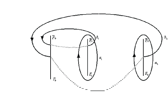
Figure 1: Cut-system.

The main result of I was the proof of the following

Theorem 2.1

Let $0\leq\delta\leq\delta_{s}(\lambda):=2\left(1+\sqrt{1+1/\lambda^{2}}\right)$ and $0<\lambda\leq\lambda_{c}$ where $\lambda_{c}(\gamma)$ is the smallest positive value of $\lambda$ for which $e^{2U_{0}}=0$. Let $E_{1}^{2}=\alpha+\mathrm{i}\beta$ with $\alpha$, $\beta$ real and

$$\alpha=-1+\frac{\delta}{2},\quad\beta=\sqrt{\frac{1}{\lambda^{2}}+\delta-\frac{\delta^{2}}{4}}.$$ (2.7)

Then the solution to the Ernst equation for an energy-momentum tensor of the form (2.5) with constant $\Omega$ and constant $\gamma$ can be written in the form

$$f(\rho,\zeta)=\frac{\Theta[m](\omega(\infty^{+})+u)}{\Theta[m](\omega(\infty^{+})-u)}e^{I},$$ (2.8)

where $I=\frac{1}{2\pi\mathrm{i}}\int\limits_{\Gamma}\ln G(\tau)d\omega_{\infty^{+}\infty^{-}}(\tau)$, where $u_{i}=\frac{1}{2\pi\mathrm{i}}\int_{\Gamma}\ln Gd\omega_{i}$, where $\Gamma$ is the covering of the imaginary axis in the +-sheet of $\Sigma_{2}$ between $-\mathrm{i}$ and $\mathrm{i}$, where the characteristic reads $[m]=\left[\begin{array}[]{cc}0&0\\ 1&1\end{array}\right]$, and where

$$G(\tau)=\frac{\sqrt{(\tau^{2}-\alpha)^{2}+\beta^{2}}+\tau^{2}+1}{\sqrt{(\tau^{2}-\alpha)^{2}+\beta^{2}}-(\tau^{2}+1)}.$$ (2.9)

We note that with $\alpha$ and $\beta$ given, the Riemann surface is completely determined at a given point in the spacetime, i.e. for a given value of $P_{0}$. In contrast to algebro-geometric solutions to non-linear evolution equations, it depends on the physical coordinates exclusively via the branch points $P_{0}$ and $\bar{P}_{0}$. Since only the modular properties of the theta functions are important, the solutions are neither periodic or quasiperiodic.

The complete metric (2.1) can be expressed via theta functions.

Theorem 2.2

Let the characteristics $[n_{i}]$ be given by $[n_{1}]=\left[\begin{array}[]{cc}0&0\\ 1&1\end{array}\right]$ and $[n_{2}]=\left[\begin{array}[]{cc}0&0\\ 0&0\end{array}\right]$. Then the function $e^{2U}$ can be written in the form

$$e^{2U}=\frac{\Theta[n_{1}](u)\Theta[n_{2}](u)}{\Theta[n_{1}](0)\Theta[n_{2}](0)}\frac{\Theta[n_{1}](\omega(\infty^{-}))\Theta[n_{2}](\omega(\infty^{-}))}{\Theta[n_{1}](\omega(\infty^{-})+u)\Theta[n_{2}](\omega(\infty^{-})+u)}e^{I}.$$ (2.10)

The metric function $a$ can be expressed via

$$\left(a-a_{0}\right)e^{2U}=-\rho\left(\frac{\Theta[n_{1}](0)\Theta[n_{2}](0)}{\Theta[n_{1}](\omega(\infty^{-}))\Theta[n_{2}](\omega(\infty^{-}))}\frac{\Theta[n_{1}](u)\Theta[n_{2}](u+2\omega(\infty^{-}))}{\Theta[n_{1}](u+\omega(\infty^{-}))\Theta[n_{2}](u+\omega(\infty^{-}))}-1\right),$$ (2.11)

where the constant $a_{0}=-\gamma/\Omega$ is determined by the condition that $a$ vanishes on the regular part of the axis and at infinity. The metric function $e^{2k}$ can be put in the form

$$e^{2k}=C\frac{\Theta[n_{1}](u)\Theta[n_{2}](u)}{\Theta[n_{1}](0)\Theta[n_{2}](0)}\exp\left(\frac{2}{(4\pi\mathrm{i})^{2}}\int_{\Gamma}\int_{\Gamma}dK_{1}dK_{2}h(K_{1})h(K_{2})\ln\frac{\Theta_{o}(\omega(K_{1})-\omega(K_{2}))}{K_{1}-K_{2}}\right),$$ (2.12)

where $\Theta_{o}$ is a theta function with an odd characteristic, where $h(\tau)=\partial_{\tau}\ln G(\tau)$, and where $C$ is a constant which is determined by the condition that $k$ vanishes on the regular part of the axis and at infinity.

Proof:
The metric potential $e^{2U}$ is just the real part of the Ernst potential. With the help of Fay’s trisecant identity [12], $e^{2U}$ was written in [8] in the form (2.10). Korotkin [6] gave an expression for the metric function $a$ as a derivative of theta functions with respect to the argument. In [8] this formula could be written in the form (2.11) free off derivatives by using the trisecant identity. The metric function $e^{2k}$ is related to the so-called $\tau$-function of the linear system associated to the Ernst equation (see [13]). This connection made it possible to give the explicit expression for $k$ in terms of theta functions of (2.12) in [14].

3 Axis and branch points

The axis of symmetry is of physical importance since the multipole moments such as the Arnowitt-Deser-Misner (ADM) mass and the angular momentum can be read off from the Ernst potential on the axis. On the axis the branch points $P_{0}$ and $\bar{P}_{0}$ coincide which implies that the Riemann surface becomes singular and that some of the periods diverge. The Ernst potential is however regular at the axis except at the disk. The proof for this result is based on results by Fay [12] and Yamada [15] and was given in [8]. We denote here and in the following the elliptic theta functions with $\vartheta_{i}$ where $i=1,\ldots,4$ for the characteristics $\left[\begin{array}[]{c}1\\ 1\end{array}\right]$, $\left[\begin{array}[]{c}1\\ 0\end{array}\right]$, $\left[\begin{array}[]{c}0\\ 0\end{array}\right]$ and $\left[\begin{array}[]{c}0\\ 1\end{array}\right]$ respectively. If one observes that $a_{0}$ and $C$ are determined by the condition that the metric functions $a$ and $k$ vanish on the regular part of the axis, one can summarize the results in the following theorem.

Theorem 3.1

We indicate quantities defined on the elliptic Riemann surface $\Sigma^{\prime}$ given by $\mu^{\prime}{}^{2}(\tau)=(\tau^{2}-\alpha)^{2}+\beta^{2}$ with a prime. Then the Ernst potential on the axis for $\zeta>0$ has the form

$$f(0,\zeta)=\frac{\vartheta_{4}(\int_{\zeta^{+}}^{\infty^{+}}d\omega^{\prime}+u_{1}^{\prime})-\exp(-\omega_{2}(\infty^{+})-u_{2})\vartheta_{4}(\int_{\zeta^{-}}^{\infty^{+}}d\omega^{\prime}+u_{1}^{\prime})}{\vartheta_{4}(\int_{\zeta^{+}}^{\infty^{+}}d\omega^{\prime}-u_{1}^{\prime})-\exp(-\omega_{2}(\infty^{+})+u_{2})\vartheta_{4}(\int_{\zeta^{-}}^{\infty^{+}}d\omega^{\prime}-u_{1}^{\prime})}e^{I^{\prime}+u_{2}},$$ (3.1)

where $d\omega_{1}=d\omega^{\prime}$, $d\omega_{2}=d\omega^{\prime}_{\zeta^{-}\zeta^{+}}$, $u_{i}=\frac{1}{2\pi\mathrm{i}}\int_{\Gamma}\ln Gd\omega_{i}$, and where $I^{\prime}=\frac{1}{2\pi\mathrm{i}}\int_{\Gamma}\ln Gd\omega^{\prime}_{\infty^{+}\infty^{-}}$. The real part of the Ernst potential can be written in the form

$$e^{2U}=\frac{\vartheta_{4}^{2}(u)}{\vartheta_{4}^{2}(0)}\frac{\vartheta_{4}^{2}\left(\int_{\zeta^{+}}^{\infty^{-}}d\omega^{\prime}\right)-\exp\left(-2\omega_{2}(\infty^{-})\right)\vartheta_{4}^{2}\left(\int_{\zeta^{-}}^{\infty^{-}}d\omega^{\prime}\right)}{\vartheta_{4}^{2}\left(u+\int_{\zeta^{+}}^{\infty^{-}}d\omega^{\prime}\right)-\exp\left(-2\omega_{2}(\infty^{-})-2u_{2}\right)\vartheta_{4}^{2}\left(u+\int_{\zeta^{-}}^{\infty^{-}}d\omega^{\prime}\right)}.$$ (3.2)

The constant $a_{0}$ can be expressed via theta functions,

$$a_{0}=\frac{\beta_{1}}{\alpha_{1}}\sqrt{\alpha_{1}^{2}+\beta_{1}^{2}}\frac{\vartheta_{4}^{4}(0)}{\vartheta_{3}^{2}(\omega(\infty^{-}))\vartheta_{4}^{2}(\omega(\infty^{-}))}\frac{\vartheta_{4}(u+2\omega(\infty^{-}))}{\vartheta_{4}(u)}e^{-I^{\prime}}.$$ (3.3)

The constant $C$ is given by

$$1/C=\frac{\vartheta_{4}^{2}(u^{\prime})}{\vartheta_{4}^{2}(0)}\exp\left(\frac{2}{(4\pi\mathrm{i})^{2}}\int_{\Gamma}\int_{\Gamma}dK_{1}dK_{2}h(K_{1})h(K_{2})\ln\frac{\vartheta_{1}(\omega^{\prime}(K_{1})-\omega^{\prime}(K_{2}))}{K_{1}-K_{2}}\right).$$ (3.4)

The Ernst potential on the axis can be used to determine the Ernst potential at the origin, $e^{2U_{0}}$, which is related to the redshift $z_{R}$ of photons emitted from the center of the disk and detected at infinity, $z_{R}=e^{-U_{0}}-1$. The surface $\Sigma^{\prime}$ admits the involution $\tau\to-\tau$ which implies $\int_{0^{+}}^{\infty^{+}}d\omega^{\prime}\equiv\frac{\pi^{\prime}}{2},\quad\int_{0^{-}}^{\infty^{+}}d\omega^{\prime}\equiv\mathrm{i}\pi$ where $\equiv$ denotes equal up to periods and where $\pi^{\prime}$ is the $b$-period on $\Sigma^{\prime}$. Similarly one has $u_{1}^{\prime}=2I^{\prime}$ and $u_{2}=\frac{1}{2}\ln G(0)+I^{\prime}$ where the integral $u_{2}$ is to be understood as the principal value (this leads to a contribution of $1/2$ times the residue). Using $e^{-\omega_{2}(\infty^{+})}=-\frac{\vartheta_{1}(\int_{0^{+}}^{\infty^{+}}d\omega^{\prime})}{\vartheta_{1}(\int_{0^{-}}^{\infty^{+}}d\omega^{\prime})}$ and $G(0)=(\sqrt{1+\lambda^{2}}+\lambda)^{2}$ one ends up with

Corollary 3.1

The Ernst potential $f_{0}$ at the center of the disk is given by

$$f_{0}=\frac{(\sqrt{1+\lambda^{2}}-\lambda)X-1}{\sqrt{1+\lambda^{2}}-\lambda+X},$$ (3.5)

where $X$ is the purely imaginary quantity

$$X=\frac{\vartheta_{3}(u_{1}^{\prime})\vartheta_{4}(0)}{\vartheta_{1}(u_{1}^{\prime})\vartheta_{2}(0)}.$$ (3.6)

The ADM mass $M$ and the angular momentum $J$ of the spacetime can be obtained by expanding the axis potential (3.1) in the vicinity of infinity. The real part of the Ernst potential for $\epsilon<1$ reads $e^{2U}=1-2M/\zeta+o(1/\zeta)$ and the imaginary part $b=2J/\zeta^{2}+o(1/\zeta^{2})$ (see e.g. [16]). We get

Corollary 3.2

The ADM mass is given by the formula

$$M=-D_{\infty^{-}}\ln\vartheta_{4}(u^{\prime})-\frac{1}{4\pi\mathrm{i}}\int_{\Gamma}\ln G\,d\omega_{1,\infty^{+}},$$ (3.7)

and the angular momentum is given by

$$J=-\frac{\gamma}{\Omega}\left(D_{\infty^{-}}\ln\vartheta_{4}(u^{\prime})+D_{\infty^{-}}\ln\vartheta_{2}(u^{\prime})+\frac{1}{2\pi\mathrm{i}}\int_{\Gamma}\ln G\,d\omega_{1,\infty^{+}}\right).$$ (3.8)

Here $D_{P}F(\omega(P))$ denotes the coefficient of the linear term in the expansion of a function $F$ in the local parameter in the vicinity of $P$.

Since we concentrate on positive values of $\zeta$, the Riemann surface can only become singular if $P_{0}$ coincides with $\bar{P}_{0}$, i.e. on the axis, or if it coincides with $E_{2}$. Then, as on the axis, several periods of the Riemann surface diverge. With the same techniques as on the axis, it was proven in [8] that the Ernst potential and the metric functions are regular at this point.

Theorem 3.2

We denote with a double prime the quantities defined on the Riemann surface $\Sigma^{\prime\prime}$ of genus 0 given by $\mu^{\prime\prime}{}^{2}(\tau)=(\tau-E_{1})(\tau-\bar{E}_{1})$. Then the differentials on $\Sigma_{2}$ reduce for $P_{0}=E_{2}$ to differentials on $\Sigma^{\prime\prime}$, $d\omega_{1}=d\omega^{\prime\prime}_{E_{2}^{-}E_{2}^{+}}$, $d\omega_{2}=d\omega^{\prime\prime}_{\bar{E}_{2}^{-}\bar{E}_{2}^{+}}$ and $I=I^{\prime\prime}=\frac{1}{2\pi\mathrm{i}}\int_{\Gamma}\ln Gd\omega^{\prime\prime}_{\infty^{+}\infty^{-}}$. The Ernst potential reads

$$f=\frac{\sinh\frac{\omega_{1}(\infty^{+})+u_{1}}{2}}{\sinh\frac{\omega_{1}(\infty^{+})-u_{1}}{2}}e^{I^{\prime\prime}},$$ (3.9)

the function $a$ follows from

$$(a-a_{0})e^{2U}$$

$$= \rho\left(\frac{\sinh\frac{\pi_{12}}{4}}{\sinh\frac{\omega_{1}(\infty^{+})}{2}\sinh\frac{\omega_{2}(\infty^{+})}{2}}\times\right.$$

$$\left.\frac{\exp\left(\frac{\pi_{12}}{4}\right)\cosh\frac{u_{1}+u_{2}+2\omega_{1}(\infty^{+})+2\omega_{2}(\infty^{+})}{2}-\exp\left(-\frac{\pi_{12}}{4}\right)\cosh\frac{u_{1}-u_{2}+2\omega_{1}(\infty^{+})-2\omega_{2}(\infty^{+})}{2}}{2\sinh\frac{u_{1}-\omega_{1}(\infty^{+})}{2}\sinh\frac{u_{2}-\omega_{2}(\infty^{+})}{2}}-1\right),$$

and the function $e^{2k}$ is given by

$$e^{2k} = C\frac{\exp\left(\frac{\pi_{12}}{4}\right)\cosh\frac{u_{1}+u_{2}}{2}-\exp\left(-\frac{\pi_{12}}{4}\right)\cosh\frac{u_{1}-u_{2}}{2}}{2\sinh\frac{\pi_{12}}{4}}$$ (3.11)

$$\exp\left(\frac{1}{(4\pi\mathrm{i})^{2}}\int_{\Gamma}\int_{\Gamma}\frac{dK_{1}dK_{2}}{(K_{1}-K_{2})^{2}}\ln G(K_{1})\ln G(K_{2})\times\right.$$

$$\left.\left(\sqrt{\frac{(K_{1}-E_{1})(K_{2}-\bar{E}_{1})}{(K_{1}-\bar{E}_{1})(K_{2}-E_{1})}}+\sqrt{\frac{(K_{1}-\bar{E}_{1})(K_{2}-E_{1})}{(K_{1}-E_{1})(K_{2}-\bar{E}_{1})}}-2\right)\right).$$

4 Metric potentials at the disk

In the equatorial plane, the Riemann surface $\Sigma_{2}$ has the additional involution $\tau\to-\tau$ which makes it possible to express the Ernst potential in terms of elliptic functions (see [8]). In I it was shown that there exist algebraic relations between the real and imaginary parts of the Ernst potential, the function $Z:=(a-a_{0})e^{2U}$ and their one-sided derivatives at the disk ($\lim_{\zeta\to 0,\zeta>0}$ and $\rho\leq 1$). The function $e^{2U}$ itself can be expressed via elliptic theta functions on the surface $\Sigma_{w}$ defined by $\mu_{w}^{2}=(\tau+\rho^{2})((\tau-\alpha)^{2}+\beta^{2})$. We cut the surface in a way that the $a$-cut is a closed contour in the upper sheet around the cut $[-\rho^{2},\bar{E}]$ and that the $b$-cut starts at the cut $[\infty,E]$. The Abel map $w$ is defined for $P\in\Sigma_{w}$ as $w(P)=\int_{\infty}^{P}dw$.

Theorem 4.1

Let $u_{w}=\frac{1}{\mathrm{i}\pi}\int_{-\rho^{2}}^{-1}\ln G(\sqrt{\tau})dw(\tau)$. Then the real part of the Ernst potential at the disk is given by

$$e^{2U} = \frac{1}{Y-\delta}\left(-\frac{1}{\lambda}-\frac{Y}{\delta}\left(\frac{\frac{1}{\lambda^{2}}+\delta}{\sqrt{\frac{1}{\lambda^{2}}+\delta\rho^{2}}}-\frac{1}{\lambda}\right)\right.$$ (4.1)

$$\left.+\sqrt{\frac{Y^{2}((\rho^{2}+\alpha)^{2}+\beta^{2})}{\frac{1}{\lambda^{2}}+\delta\rho^{2}}-2Y(\rho^{2}+\alpha)+\frac{1}{\lambda^{2}}+\delta\rho^{2}}\right),$$

where

$$Y=\frac{\frac{1}{\lambda^{2}}+\delta\rho^{2}}{\sqrt{(\rho^{2}+\alpha)^{2}+\beta^{2}}}\frac{\vartheta_{3}^{2}(u_{w})}{\vartheta_{1}^{2}(u_{w})}.$$ (4.2)

At the disk, the relations

$$\frac{\delta^{2}}{2}(e^{4U}+b^{2})=\left(\frac{1}{\lambda}-\delta e^{2U}\right)\left(\frac{\frac{1}{\lambda^{2}}+\delta}{\sqrt{\frac{1}{\lambda^{2}}+\delta\rho^{2}}}-\frac{1}{\lambda}\right)+\delta\left(\frac{\delta+\rho^{2}}{2}-1\right),$$ (4.3)

for $e^{2U}$ and $b$,

$$Z^{2}-\rho^{2}+\delta e^{4U}=\frac{2}{\lambda}e^{2U}$$ (4.4)

for $Z$ and $e^{2U}$, and

$$\left(e^{2U}\right)_{\zeta}=\frac{Z^{2}+\rho^{2}+\delta e^{4U}}{2Z\rho}b_{\rho}$$ (4.5)

for the derivatives are valid.

Proof:
One can define on $\Sigma_{w}$ the divisor $W$ as the solution of the Jacobi inversion problem

$$\int_{\infty}^{W}dw:=u_{w}.$$ (4.6)

Thus $W$ can be expressed in standard manner via theta functions on $\Sigma_{w}$,

$$W+\rho^{2}=\sqrt{(\rho^{2}+\alpha)^{2}+\beta^{2}}\frac{\vartheta_{3}^{2}(u_{w})}{\vartheta_{1}^{2}(u_{w})}.$$ (4.7)

In I it was shown that $W$ is related to $e^{2U}$,

$$W+\rho^{2}=\frac{\delta^{2}((\rho^{2}+\alpha)^{2}+\beta^{2})}{2\left(\frac{1}{\lambda^{2}}+\delta\rho^{2}\right)}\frac{\rho^{2}+\frac{2}{\lambda}e^{2U}-\delta e^{4U}}{\left(\frac{1}{\lambda}-\delta e^{2U}\right)\left(\frac{\frac{1}{\lambda^{2}}+\delta}{\sqrt{\frac{1}{\lambda^{2}}+\delta\rho^{2}}}-\frac{1}{\lambda}\right)+\frac{\delta}{2}(\rho^{2}+2\alpha)-\frac{\delta^{2}}{2}e^{4U}}.$$ (4.8)

Entering with this relation in (4.7) and solving for $e^{2U}$, one ends up after some algebraic manipulation with (4.1). The relations (4.3) to (4.5) were given in I. This completes the proof.

To discuss physical quantities in the disk, the behaviour of the metric in the vicinity of the center and of the rim of the disk is important. We have

Corollary 4.1

At the disk ($\zeta\to 0$, $\zeta>0$), the metric functions and their derivatives have for $\rho\to 0$ and $\lambda<\lambda_{c}$, $\delta\leq\delta_{s}(\lambda)$ an expansion of the form $F=F_{0}+F_{2}\rho^{2}+F_{4}\rho^{4}+\ldots$ where $F$ stands for $e^{2U}$, $Z$, $b$, $\left(e^{2U}\right)_{\zeta}$, and $e^{2k}$, and where the $F_{i}$ are constants with $b_{0}^{2}=1-4\Omega^{2}-e^{4U_{0}}$ and $Z_{0}=(\gamma/\Omega)e^{2U_{0}}$.
For $\delta=0$ and $\lambda=\lambda_{c}$ the metric functions and their derivatives have an expansion of the form $e^{2U}=-\frac{\lambda}{2}\rho^{2}+\rho^{4}y_{4}+\ldots$, $Z=\rho^{2}Z_{2}+\ldots$, $b=-1+\rho^{4}\lambda y_{4}+\ldots$, $\left(e^{2U}\right)_{\zeta}=-\sqrt{2\lambda y_{4}}\rho^{2}+\ldots$,and $k=\ln\rho+k_{0}+k_{2}\rho^{2}+\ldots$.
For $\delta\neq 0$, the critical value $\lambda_{c}\to\infty$. In this case the expansion of the metric functions is as for $\delta=0$, $\lambda=\lambda_{c}$ or of the form $e^{2U}=y_{1}\rho+\rho^{3}y_{3}+\ldots$, $Z=Z_{1}\rho+\rho^{3}Z_{3}+\ldots$, $b=b_{0}+\rho^{2}b_{2}+\ldots$, $\left(e^{2U}\right)_{\zeta}=s_{1}\rho+\ldots$, $k=\frac{1}{4}\ln\rho+k_{0}+k_{2}\rho^{2}+\ldots$.
At the rim of the disk ($\rho=1$), the imaginary part of the Ernst potential vanishes for $\delta>\delta_{s}$ and $\rho\leq 1$ as $(1-\rho^{2})^{\frac{3}{2}}$.

Proof:
Since the Riemann surface $\Sigma_{w}$ is regular for $0\leq\rho\leq 1$, all periods are functions of $\rho^{2}$. The integral $u_{w}$ is also a smooth function of $\rho^{2}$ which can be seen from

$$\frac{1}{\mathrm{i}\pi}\int_{-\rho^{2}}^{-1}\frac{\ln G(\sqrt{\tau})d\tau}{\sqrt{(\tau+\rho^{2})((\tau-\alpha)^{2}+\beta^{2})}}=\frac{2}{\pi}\sqrt{1-\rho^{2}}\int_{0}^{1}\tilde{G}((1-\rho^{2})t+\rho^{2})dt,$$ (4.9)

where

$$\tilde{G}(\tau)=\frac{2\ln(\sqrt{(\tau+\alpha)^{2}+\beta^{2}}+1-\tau)-\ln\left(\frac{1}{\lambda^{2}}+\delta\tau\right)}{\sqrt{(\tau+\alpha)^{2}+\beta^{2}}}.$$ (4.10)

Thus the quantity $Y$ in (4.2) is a smooth function in $\rho^{2}$. For $\lambda<\lambda_{c}$ it has the form $Y(\rho)=Y_{0}+Y_{2}\rho^{2}+\ldots$ This implies via the relations of Theorem 4.1 that $e^{2U}$, $Z$, $b$ and $\left(e^{2U}\right)_{\zeta}$ are also smooth functions in $\rho^{2}$. The behaviour of $k$ is determined by using the relation (2.4) together with the condition that $k$ vanishes on the axis.
In the case $\gamma=1$ the ultra-relativistic limit $e^{2U_{0}}=1$ is reached for $\vartheta_{3}(u_{w})=0$ for $\rho=0$ i.e. $Y=0$ at the center of the disk. Since the theta functions in (4.2) are functions in $\rho^{2}$ and since $Y$ is quadratic in the theta functions, $Y$ is of the form $Y=Y_{4}\rho^{4}+\ldots$. Expanding $e^{2U}$ in (4.1) for small $Y$ one gets $e^{2U}=-\frac{\lambda}{2}\rho^{2}+\frac{\lambda}{2}Y$. For $\lambda\to\infty$ and $0<\gamma<1$, equation (4.1) leads to $e^{2U}=\rho y_{1}+\rho^{3}y_{3}+\ldots$ for $y_{1}\neq 0$ or $e^{2U}=\rho^{2}y_{2}+\rho^{4}y_{4}+\ldots$ for $y_{1}=0$. For $y_{1}\neq 0$ relation (4.3) can either be satisfied by a function $b$ of the form $b=b_{0}+b_{2}\rho^{2}+\ldots$ or $b=b_{1}\rho+\ldots$. To decide one has to consider $b_{0}$ which has the form $\frac{\delta}{2}b_{0}^{2}=\alpha-\theta+\sqrt{\theta^{2}-2\alpha\theta+1}$, where $\theta=\vartheta_{2}^{2}(u_{w})/\vartheta_{1}^{2}(u_{w})$ for $\rho=0$. Thus $b_{0}$ can only vanish for $\delta\neq 0$ in this case if $\delta=4$, the static limit, where it vanishes identically.
The behaviour of $b$ at the rim of the disk follows from (4.3) which implies with (4.1)

$$b^{2} = \frac{2}{(Y-\delta)^{2}}\left(\delta\alpha-\frac{1}{\lambda^{2}}-Y\left(\alpha+\frac{2-\rho^{2}+\delta\lambda^{2}}{1+\lambda^{2}\delta\rho^{2}}\right)+\right.$$ (4.11)

$$\left.\frac{\frac{1}{\lambda^{2}}+\delta}{\sqrt{\frac{1}{\lambda^{2}}+\delta\rho^{2}}}\sqrt{\frac{Y^{2}((\rho^{2}+\alpha)^{2}+\beta^{2})}{\frac{1}{\lambda^{2}}+\delta\rho^{2}}-2Y(\rho^{2}+\alpha)+\frac{1}{\lambda^{2}}+\delta\rho^{2}}\right).$$

Since the Riemann surface $\Sigma_{w}$ and therefore its periods are regular at $\rho=1$, the integral $u_{w}$ is dominated by the integral in (4.9) which is proportional to $(1-\rho^{2})^{\frac{3}{2}}$ for $\rho\approx 1$ in the disk. The theta function $\vartheta_{1}(x)$ has zeros of first order at $x=0$ which implies that $Y$ diverges for $\rho\to 1$. Consequently for $\rho\approx 1$ we have $b^{2}\approx\frac{2}{Y}\left(\sqrt{\frac{1}{\lambda^{2}}+\delta}-\frac{\delta}{2}\right)$which implies that $b\propto\vartheta_{1}(u_{w})$ i.e. $b\propto(1-\rho^{2})^{\frac{3}{2}}$ in the non-static case.

5 Limiting cases

The one-component disk which was studied by Bardeen and Wagoner [20] is obtained by simply putting $\delta=0$ in the Ernst potential (2.8). This gives the solution of Neugebauer and Meinel [5] in the notation of [7, 8].

5.1 Newtonian limit

The Newtonian limit is reached for $\lambda\to 0$ for arbitrary $\delta$ which follows from (2.6): If $e^{-U_{0}}-1\ll 1$ and $\Omega=\Omega\rho_{0}\ll 1$, this means that both the central redshift and the maximal velocity in the disk (compared to the velocity of light which is 1 in the used units) are small, which just defines the Newtonian regime. We get

Theorem 5.1

In the limit $\lambda\ll 1$, the Ernst potential (2.8) becomes real with $U$ given by

$$U(\rho,\zeta)=-\frac{1}{4\pi\mathrm{i}}\int_{-\mathrm{i}}^{\mathrm{i}}\frac{2\lambda(\tau^{2}+1)}{\sqrt{(\tau-\zeta)^{2}+\rho^{2}}}d\tau.$$ (5.1)

The metric functions $a$ and $k$ are of order $\Omega^{3}$ and $\Omega^{4}$ respectively.

Equation (5.1) just describes the Maclaurin disk in the notation of I. The metric has the behaviour one expects from a general post-Newtonian expansion.
Proof:
In the limit $\lambda\to 0$, the branch points $E_{i}$ and $\bar{E}_{i}$, $i=1,2$, tend to infinity. To treat this limiting case, we use the conformal transformation $\tau\to\tau/\sqrt{\lambda}$. On the transformed surface, the cut $[\sqrt{\lambda}P_{0},\sqrt{\lambda}\bar{P}_{0}]$ collapses as on the axis, whereas the remaining cuts remain finite. In the limit $\lambda\to 0$ the Abelian integrals can be expressed in terms of quantities on the elliptic Riemann surface $\tilde{\Sigma}$ given by $\tilde{\mu}{}^{2}(\tau)=\tau^{4}+1$. We get

$$f=e^{I-u_{1}-u_{2}}\frac{\vartheta_{3}(u_{1})\vartheta_{4}(0)-\vartheta_{2}(0)\vartheta_{1}(u_{1})\exp\left(u_{2}+\frac{u_{1}}{2}\right)}{\vartheta_{3}(u_{1})\vartheta_{4}(0)+\vartheta_{2}(0)\vartheta_{1}(u_{1})\exp\left(-u_{2}-\frac{u_{1}}{2}\right)}.$$ (5.2)

The $u_{i}$ and $I$ are however not Abelian integrals. We have $\oint_{a_{1}}\frac{\tau^{n}d\tau}{\mu(\tau)}\propto\lambda^{1-\frac{n}{2}}$, whereas the corresponding $a_{2}$-periods are proportional to $\lambda$. With $\ln G\approx 2\lambda(\tau^{2}+1)$ we thus find that $u_{1}$ and $I$ are proportional to $\lambda^{\frac{3}{2}}$ and $u_{2}=\frac{1}{2\pi\mathrm{i}}\int_{\Gamma}\frac{2\lambda(\tau^{2}+1)d\tau}{\sqrt{(\tau-\zeta)^{2}+\rho^{2}}}$ in lowest order.

The leading contributions in (5.2) are consequently given by $u_{2}$ in $f=1-u_{2}$. Since $f=e^{2U}$ in this case, we get (5.1). In a similar way the lowest order contributions to the imaginary part can be obtained from (5.2). They arise from the term $\vartheta_{1}(u_{1})$ which is an odd and purely imaginary function. It has zeros of first order which implies that $b\propto u_{1}$ which is of order $\lambda^{\frac{3}{2}}$ i.e. of order $\Omega^{3}$. Thus $a$ is also of order $\Omega^{3}$. For the metric function $k$ we get with (2.12) as above that the leading contributions arise from the integral in the exponent which are quadratic in $G$ and thus of order $\Omega^{4}$. This completes the proof.

5.2 Static limit

The static limit of the Ernst potential (2.8) is obtained for $\beta=0$, i.e. $\delta_{s}(\lambda)=2(1+\sqrt{1+1/\lambda^{2}})$. We get

Theorem 5.2

The function (2.8) becomes real in the limit $\delta=\delta_{s}(\lambda)$ with the potential $U$ given by

$$U(\rho,\zeta)=-\frac{1}{4\pi\mathrm{i}}\int_{-\mathrm{i}}^{\mathrm{i}}\ln G\frac{d\tau}{\sqrt{(\tau-\zeta)^{2}+\rho^{2}}},\quad G=\left(1-\frac{4}{\delta}(\tau^{2}+1)\right).$$ (5.3)

The metric function $a$ vanishes identically whereas the function $k$ is given by

$$k = \frac{1}{2(4\pi\mathrm{i})^{2}}\int_{\Gamma}\int_{\Gamma}dK_{1}dK_{2}\ln G(K_{1})\ln G(K_{2})$$ (5.4)

$$\frac{1}{(K_{1}-K_{2})^{2}}\left(\sqrt{\frac{(K_{1}-i\bar{z})(K_{2}+iz)}{(K_{2}-i\bar{z})(K_{1}+iz)}}+\sqrt{\frac{(K_{2}-i\bar{z})(K_{1}+iz)}{(K_{1}-i\bar{z})(K_{2}+iz)}}-2\right).$$

This is the static disk of Morgan and Morgan [17] with uniform rotation.

Proof:
In the limit $\delta\to\delta_{s}$, the branch points $E_{i}$ and $\bar{E}_{i}$ coincide for $i=1,2$ on the real axis since $\delta_{s}\geq 4$ and thus $\alpha(\delta_{s})=\delta_{s}/2-1>0$. Mathematically this limit corresponds to the standard solitonic limit of algebro-geometric solutions of evolution equations, see e.g. [18]. In the cut-system Fig. 1 the $b$-periods $\pi_{11}$ and $\pi_{22}$ diverge whereas the remaining periods are finite. Thus in this limit the theta functions in (2.8) become identical to 1 whereas the differential of the third kind $d\omega_{\infty^{+}\infty^{-}}\to-\frac{d\tau}{\sqrt{(\tau-\zeta)^{2}+\rho^{2}}}$. The limit of (2.9) for $\delta=\delta_{s}$ is (5.3) which is identical to $\ln G=4U_{0}+\ln\left(1+2\lambda e^{-2U_{0}}\tau^{2}\right)$, i.e. the form which was given for the Morgan and Morgan disk with constant $\Omega$ in [19]. Since the theta functions in (2.11) all tend to one, we find that $a$ is identical to zero in this case with $a_{0}=-\gamma/\Omega$ being equal to zero for $\gamma=0$. In the expression for the metric function $k$ (2.12) the theta functions again tend to 1. To evaluate the integral in the exponent, we integrate by parts with respect to both $K_{1}$ and $K_{2}$ using the fact that $\ln G$ vanishes at the limits of integration. The differential of the second kind then takes the form given in (5.4). Since $k$ obviously vanishes on the axis, the constant $C$ is identical to 1 in this limit. This completes the proof.

5.3 Ultra-relativistic limit

The ultra-relativistic limit is reached if the redshift of photons emitted at the center of the disk and detected at infinity diverges which is equivalent to the fact that photons from the center of the disk cannot escape to infinity as from a horizon of a black-hole. In the case $\gamma=1$ the limit is reached for $\vartheta_{4}(u^{\prime})=0$. This implies with (3.3) and (3.4) that both constants $a_{0}$ and $C$ diverge as $\epsilon\to 1$. The axis is in fact singular in the sense that the metric function $e^{2U}$ vanishes there identically which can be seen from (3.2). The Ernst potential is identical to $-\mathrm{i}$ on the axis for $\zeta>0$. A consequence of the diverging constant $a_{0}$ is that the angular velocity $\Omega=\Omega\rho_{0}$, which is the coordinate angular velocity in the disk as measured from infinity, vanishes. Since this implies that either $\rho_{0}$ or $\Omega$ vanish, Bardeen and Wagoner [20] argued that the spacetime can be interpreted in the limit $\epsilon\to 1$ and $\rho_{0}\to 0$ as the extreme Kerr metric in the exterior of the disk. In [7] it was shown that such a limit (diverging multipoles, singular axis,…) can occur in general hyperelliptic solutions and can always be interpreted as an extreme Kerr spacetime. For an algebraic treatment of the ultra-relativistic limit of the Bardeen-Wagoner disk see [21]. We have

Theorem 5.3

Let $f$ be an Ernst potential of the form (2.8), which is regular except at the disk, with $\vartheta_{4}(u^{\prime})=0$ and $\lim_{\rho_{0}\to 0}\rho_{0}a_{0}=:-2m$ where $m$ is a finite non-zero positive real constant. Then in the limit $\rho_{0}\to 0$, the Ernst potential (2.8) for $\rho^{2}+\zeta^{2}\neq 0$ takes the form

$$f=\frac{\rho^{2}+\zeta^{2}+m(\mathrm{i\zeta-\sqrt{\rho^{2}+\zeta^{2}}})}{\rho^{2}+\zeta^{2}+m(\mathrm{i\zeta+\sqrt{\rho^{2}+\zeta^{2}}})}.$$ (5.5)

In the ultra-relativistic limit of the above disks for $\gamma=1$, this implies that the spacetime becomes an extreme Kerr spacetime with $m=\frac{1}{2\Omega}$.
Proof:
The most direct way to prove this statement seems to determine the potential in the limit on the axis and then to use a theorem of Hauser and Ernst [23] that an Ernst potential is uniquely determined for given sources if it is given on some finite regular part of the axis. The potential on the axis is given by (3.1). The limit $\rho_{0}\to 0$ is equivalent to the limit $\zeta\to\infty$ as used in the calculation of the ADM-mass and the angular momentum in section 3 with $\vartheta_{4}(u^{\prime})=0$. The constant $a_{0}$ can be written with the help of Fay’s trisecant identity [12] as

$$a_{0}=-2\mathrm{i}\frac{D_{\infty^{-}}\vartheta_{1}(0)\vartheta_{4}(u^{\prime}+2\omega(\infty^{-}))}{\vartheta_{1}(2\omega(\infty^{-}))\vartheta_{4}(u^{\prime})},$$ (5.6)

This implies with identities between elliptic theta functions (see e.g. [24]) and the fact that $u^{\prime}\equiv\pi^{\prime}/2$, the $b$-period on $\Sigma^{\prime}$, that $a_{0}=-2D_{\infty^{-}}\ln\vartheta_{4}(u^{\prime})$. Expanding the axis potential (3.1) in first order of $\rho_{0}$, one thus gets

$$f(0,\zeta)=\frac{\zeta+m(\mathrm{i}-1)}{\zeta+m(\mathrm{i}+1)},$$ (5.7)

which is the potential (5.5) on the axis. This completes the proof.

For $\gamma<1$ the axis remains regular except at the origin, the constants $a_{0}$ and $C$ in (3.3) and (3.4) remain finite here since they can only diverge if $\vartheta_{4}(u^{\prime})=0$ which can happen only for $\gamma=1$. The integrals in the respective exponents of (3.3) and (3.4) are always finite though $\ln G(\tau)$ has a term $\ln\tau$ in the limit $\lambda\to\infty$ as can be easily seen. The ultrarelativistic limit of the disks with counter-rotation is thus a disk of finite radius with diverging central redshift.

Acknowledgment
I thank R. Kerner, D. Korotkin, H. Pfister, O. Richter and U. Schaudt for helpful remarks and hints. This work was supported by the Marie-Curie program of the European Community.

References

• [1] F. J. Ernst, Phys. Rev, 167, 1175; Phys. Rev 168, 1415 (1968).
• [2] D. Maison, Phys. Rev. Lett., 41, 521 (1978).
• [3] V. A. Belinski and V. E. Zakharov, Sov. Phys.–JETP, 48, 985 (1978).
• [4] G. Neugebauer, J. Phys. A: Math. Gen., 12, L67 (1979).
• [5] G. Neugebauer and R. Meinel, Astrophys. J., 414, L97 (1993); Phys. Rev. Lett., 73, 2166 (1994); Phys. Rev. Lett., 75, 3046 (1995).
• [6] D. A. Korotkin, Theor. Math. Phys. 77, 1018 (1989); Commun. Math. Phys., 137, 383 (1991); Class. Quant. Grav., 10, 2587 (1993).
• [7] C. Klein and O. Richter, Phys. Rev. Lett., 79, 565 (1997).
• [8] C. Klein and O. Richter, Phys. Rev. D, 58, CID 124018 (1998).
• [9] C. Klein and O. Richter, Phys. Rev. Lett., 83, 2884 (1999).
• [10] C. Klein, to be published in Phys. Rev. D, (2000).
• [11] D. Kramer, H. Stephani, E. Herlt and M. MacCallum, Exact Solutions of Einstein’s Field Equations, Cambridge: CUP, (1980).
• [12] J. Fay, Theta functions on Riemann surfaces, Lecture Notes on Mathematics Vol. 352 (Springer, New York, 1973).
• [13] D. Korotkin and H. Nicolai, Nucl. Phys. B, 475, 397 (1996).
• [14] D. Korotkin and V. Matveev, Funct. Anal. Appl., 34 1 (2000).
• [15] A. Yamada, Kodai Math. J., 3, 114 (1980).
• [16] R. Wald, General Relativity, Chicago, London: The University of Chicago Press (1984).
• [17] T. Morgan and L. Morgan Phys. Rev., 183, 1097 (1969); Errata: 188, 2544 (1969).
• [18] D. Mumford, Tata Lectures on Theta II, Progress in Mathematics Vol. 43 (Birkhäuser, Boston, 1993).
• [19] C. Klein, Class. Quant. Grav., 14, 2267 (1997).
• [20] J. M. Bardeen and R. V. Wagoner, Ap. J., 167, 359 (1971).
• [21] R. Meinel, gr-qc/9703077 (1997).
• [22] D. Korotkin and V. Matveev, Lett. Math. Phys., 49, 145 (1999).
• [23] I. Hauser and F. Ernst, J. Math. Phys., 21, 1126 (1980).
• [24] E.D. Belokolos, A.I. Bobenko, V.Z. Enolskii, A.R. Its and V.B. Matveev, Algebro-Geometric Approach to Nonlinear Integrable Equations, Berlin: Springer, (1994).