Strong field limit of black hole gravitational lensing

Abstract

We give the formulation of the gravitational lensing theory in the strong field limit for a Schwarzschild black hole as a counterpart to the weak field approach. It is possible to expand the full black hole lens equation to work a simple analytical theory that describes at a high accuracy degree the physics in the strong field limit. In this way, we derive compact and reliable mathematical formulae for the position of additional critical curves, relativistic images and their magnification, arising in this limit.

PACS numbers: 95.30.Sf, 04.70.-s, 98.62.Sb

I Introduction

The simplicity of the theory of gravitational lensing derives from some basic assumptions which are satisfied by most physical situations [1]. Through the weak field and the thin lens approximations, the whole theory was built and succeeded in explaining the phenomenology risen up to now.

Yet, gravitational lensing must not be conceived as a weak field phenomenon, since high bending and looping of light rays in strong fields is one of the most well-known and amazing predictions of general relativity. The importance of gravitational lensing in strong fields is highlighted by the possibility of testing the full general relativity in a regime where the differences with non-standard theories would be manifest, helping the discrimination among the various theories of gravitation [2]. However, the complexity of the full mathematical treatment and the difficulties of experimental or observational evidences are obstacles for these studies.

Without the linear approximations, we have trascendent equations which are hard to be handled even numerically.

Several studies about light rays close to the Schwarzschild horizon has been lead: for example, Viergutz [3] made a semi–analytical investigation about geodesics in Kerr geometry; in refs. [4, 5] the appearance of a black hole in front of a uniform background was studied. Recently, Virbhadra & Ellis [6] faced the simplest strong field problem, represented by deflection in Schwarzschild space–time, by numerical techniques. The existence of an infinite set of relativistic images has been enlightened and the results have been applied to the black hole at the centre of the Galaxy. Later on, by an alternative formulation of the problem, Frittelli, Kling & Newman [7] attained an exact lens equation, giving integral expressions for its solutions, and compared their results to those by Virbhadra & Ellis.

All these studies are affected by the high complexity in the investigation of the geodesics in the neighbourhood of the horizon and must resort to numerical methods to return valuable results. This issue prevents any kind of general and systematic investigation of light bending in this region, since fair analytical formulae for the interesting quantities are absolutely missing.

Starting from the black hole lens equation of ref. [6], we perform a set of expansions exploiting the source–lens–observer geometry and the properties of highly deflected light rays. In this way, we manage to solve the lens equation and find analytical expressions for the infinite set of images formed by the black hole. This approach leads to extremely simple formulae which allow an immediate comprehension of the problem and a straightforward application to the physically interesting situations. This strong field approach can be surely considered as the direct counterpart of the weak field limit for its striking simplicity and reliability. On the other hand, this approach allows to investigate where the strong field limit effects become relevant.

This paper is structured as follows: In Sect. 2, the black hole lens equation is presented and the first basic approximations are explained. Sect. 3 contains the calculation of the deflection angle. In Sect. 4 the deflection angle is then plugged in the black hole lens equation to derive the relativistic images, their amplification and the critical curves. Sect. 5 contains a discussion of these results. Conclusions are drawn in Sect. 6.

II The black hole lens equation

The geometrical configuration of gravitational lensing is shown in Fig. 1. The light emitted by the source $S$ is deviated by the black hole $L$ and reaches the observer $O$. Here, as a black hole, we mean any compact object having a radius comparable to its Schwarzschild radius, so that even very compact object which has not undergone a full gravitational collapse would work in the same way; $\beta$ is the angular position of the source with respect to the optical axis $OL$ and $\theta$ is the angular position of the image seen by the observer. It is important to stress that the closest approach distance $x_{0}$ does not coincide with the impact parameter $b$, unless in the limit of vanishing deflection angle $\alpha$.

By inspection of Fig. 1, it is possible to write a relation among the source position, the image position and the deflection angle $\alpha$.

$$\tan\beta=\tan\theta-\frac{D_{LS}}{D_{OS}}\left[\tan\theta+\tan\left(\alpha-\theta\right)\right].$$ (1)

This is what is called the full lens equation. Given a source position $\beta$, the values of $\theta$, solving this equation, give the position of the images observed by $O$.

In the weak field limit, several standard approximations are performed. The tangents are expanded to the first order in the angles since they are, at most, of the order of arcsec. The weak field assumption reduces the deflection angle to ${\displaystyle\frac{4GM}{c^{2}x_{0}}}$. Then the lens equation can be solved exactly and two images are found: one on the same side of the source and one on the opposite. Their separations from the optical axis are of the order of the Einstein angle

$$\theta_{E}=\sqrt{\frac{4GM}{c^{2}}\frac{D_{LS}}{D_{OS}D_{OL}}}.$$ (2)

It is easy to see that, in most relevant cases, these images are formed by light rays passing very far from the event horizon, justifying the weak field approximation [1].

Now we turn to the study of gravitational lensing in strong field. From now on, all lengths will be expressed in units of the Schwarzschild radius ${\displaystyle\frac{2GM}{c^{2}}}$. The deflection angle $\alpha$ contains the physical information about the deflector and must be calculated through the integration of the geodesic of the light ray [8]. Its integral expression, as a function of $x_{0}$, is

$$\alpha\left(x_{0}\right)=\int\limits_{x_{0}}^{\infty}\frac{2}{x\sqrt{\left(\frac{x}{x_{0}}\right)^{2}\left(1-\frac{1}{x_{0}}\right)-\left(1-\frac{1}{x}\right)}}{d}x-\pi.$$ (3)

The next section is completely devoted to the achievement of a manageable expression for this quantity as a function of $\theta$.

When the light ray trajectory gets closer to the event horizon, the deflection increases. At some impact parameter, $\alpha$ becomes higher than $2\pi$, resulting in a complete loop of the light ray around the black hole. Decreasing further the impact parameter, the light ray winds several times before emerging. Finally, for $b=(3\sqrt{3})/2$, corresponding to $x_{0}=3/2$, the deflection angle diverges and the light ray is captured by the black hole. For each loop we add to the light ray geodesic, there is one particular value of the impact parameter such that the observer is reached by the light coming from the source. So there will be an infinite sequence of images on each side of the lens.

We shall put our attention on situations where the source is almost perfectly aligned with the lens. In fact, this is the case where the relativistic images are most prominent. In this case, we are allowed to expand $\tan\beta$ and $\tan\theta$ to the first order. Some more words are needed for the term $\tan\left(\alpha-\theta\right)$. Even if $\theta$ is small, $\alpha$ is not small in the situations of our interest. However, if a ray of light emitted by the source $S$ is going to reach the observer after turning around the black hole, $\alpha$ must be very close to a multiple of $2\pi$. Writing $\alpha=2n\pi+\Delta\alpha_{n}$, with $n$ integer, we can perform the expansion $\tan\left(\alpha-\theta\right)\sim\Delta\alpha_{n}-\theta$. The lens equation becomes

$$\beta=\theta-\frac{D_{LS}}{D_{OS}}\Delta\alpha_{n}.$$ (4)

As defined by (3), $\alpha$ is a positive real number, corresponding to a clockwise winding in Fig. 1. We have inserted it in (4) without giving a sign. Taking a positive $\beta$, this equation describes only images on the same side of the source ($\theta>0$). To obtain the images on the opposite side, we can solve the same equation with the source placed in $-\beta$. Taking the opposite of these solutions, we obtain the full set of the secondary images.

III The deflection angle

The deflection angle can be evaluated exactly, but its expression does not allow the resolution of (4). Anyway, it is possible to make some simplifying but very general approximations which reduce the deflection angle to an expression easier to handle. By this strategy, we shall calculate this fundamental quantity. All approximations are essentially based on the proximity of the closest approach distance $x_{0}$ to its minimum value which is $3/2$.

The integral in Eq.(3) gives the following result

$$\alpha=-\pi-4F\left(\phi_{0},\lambda\right)G\left(x_{0}\right)$$ (5)

where

$$G\left(x_{0}\right)=\sqrt{\frac{x_{0}\left(-3+3x_{0}-\sqrt{-3+2x_{0}+x_{0}^{2}}\right)}{\left(3-2x_{0}\right)\left(1-x_{0}+\sqrt{-3+2x_{0}+x_{0}^{2}}\right)}}$$ (6)

and

$$F\left(\phi_{0},\lambda\right)=\int\limits_{0}^{\phi_{0}}\left(1-\lambda\sin^{2}\phi\right)^{-1/2}{d}\phi$$ (7)

is an elliptic integral of first kind. The parameters $\phi_{0}$ and $\lambda$ themselves are functions of $x_{0}$:

$$\phi_{0}=\arcsin\sqrt{\frac{-3+x_{0}-\sqrt{-3+2x_{0}+x_{0}^{2}}}{2\left(-3+2x_{0}\right)}},$$ (8)

and

$$\lambda=\frac{3-x_{0}-\sqrt{-3+2x_{0}+x_{0}^{2}}}{3-x_{0}+\sqrt{-3+2x_{0}+x_{0}^{2}}}.$$ (9)

Fig. 2 shows a plot of the deflection angle. This expression is, of course, too complicated to use in Eq. (4). However, we can see that $\alpha$ diverges when $x_{0}\rightarrow 3/2$. On the other hand, we are interested just into small closest approaches, since they correspond to the high deflection angles producing relativistic images. If we let $x_{0}=3/2+\epsilon$, we can search for the leading order term in the divergence when $\epsilon\rightarrow 0$.

After some non–trivial expansions, we find that the leading order of the deflection angle is logarithmic in $\epsilon$, that is

$$\alpha\sim-2\log\frac{\left(2+\sqrt{3}\right)\epsilon}{18}-\pi.$$ (10)

In Fig. 3, we plot the ratio of the exact deflection angle and its leading order expansion. Of course, the two functions coincide in the limit $x_{0}\rightarrow 1.5$. Using our expansion up to $x_{0}=1.55$, the error we commit is about $1\%$. For our purposes, this is largely sufficient as we shall see later.

The next step is to convert the dependence on $x_{0}$ into a dependence on the impact parameter $b$ and then on $\theta$. The study of light ray dynamics in Schwarzschild metric gives the relation [8]

$$x_{0}^{2}=\left(1-\frac{1}{x_{0}}\right)b^{2}.$$ (11)

For values of $x_{0}$ close to $3/2$, this relation can be solved perturbatively (or, equivalently, one can expand the exact root of the third degree polynomial equation in $x_{0}$ to the first non-trivial order), giving the relation

$$\epsilon=\sqrt{\frac{b-\frac{3\sqrt{3}}{2}}{\sqrt{3}}}.$$ (12)

Remembering that $b\simeq\theta D_{OL}$, we can substitute this relation into Eq. (10) to retrieve $\alpha$ as a function of $\theta$, that is

$$\alpha\sim-\log\left(\theta D_{OL}-\frac{3\sqrt{3}}{2}\right)+A,$$ (13)

with

$$A=-\log\frac{\left(5+3\sqrt{3}\right)}{1944}-\pi=2.109.$$ (14)

Eq. (13) is the highly simplified expression for the deflection angle we were looking for. It allows reliable calculations, as we shall see in the next section, where we insert it in the lens equation.

IV Images, magnification, critical curves

According to the considerations done at the end of Sect. 2, what enters the lens equation is not the full deflection angle but its deviation from a multiple of $2\pi$. First of all, we have to find the values of $\theta$ (denoted by $\theta_{n}^{0}$) such that

$$\alpha\left(\theta_{n}^{0}\right)=2n\pi.$$ (15)

Inverting this equation, with $\alpha$ given by (13), we have

$$\theta_{n}^{0}=\frac{3\sqrt{3}+2e^{A-2n\pi}}{2D_{OL}}.$$ (16)

As expected, if we let the number of loops around the black hole tend to infinity, we have ${\displaystyle\theta_{\infty}^{0}=\frac{3\sqrt{3}}{2D_{OL}}}$. $\theta_{n}^{0}$ are the starting points for all the successive calculations. The offsets $\Delta\alpha_{n}$ can be found by expanding $\alpha$ to the first order in $\Delta\theta_{n}=\theta-\theta_{n}^{0}$:

$$\Delta\alpha_{n}=-\frac{D_{OL}}{e^{A-2n\pi}}\Delta\theta_{n}.$$ (17)

We have all the ingredients to solve the lens equation (4), which becomes

$$\beta=\left(\theta_{n}^{0}+\Delta\theta_{n}\right)+\left(\frac{D_{OL}}{e^{A-2n\pi}}\frac{D_{LS}}{D_{OS}}\right)\Delta\theta_{n}.$$ (18)

We can observe that $D_{OL}$, $D_{LS}$, $D_{OS}$ are all much greater than unity (remember that all distances are measured in Schwarzschild radii) and $e^{A-2\pi}=3.25\times 10^{-3}$. This means that the last term in Eq.(18) prevails on the $\Delta\theta_{n}$ at the second place in the rhs. Neglecting this term, we finally get the position of the $n^{th}$ image as

$$\theta_{n}\simeq\theta_{n}^{0}+\frac{e^{A-2n\pi}\left(\beta-\theta_{n}^{0}\right)D_{OS}}{D_{LS}D_{OL}}.$$ (19)

We see that, when $\beta$ equals $\theta_{n}^{0}$, there is no correction to the position of the $n^{th}$ image, that remains in $\theta_{n}^{0}$ simply. In this particular case, the image position coincides with the source position. It is worthwhile to note that the second term in (19) is much smaller than the first one. For practical purposes, $\theta_{n}^{0}$ are already a good approximation for the position of relativistic images.

The relation (17) can help us to estimate the error in the determination of the position of the images. We do this in the least favorable case that is for the first image, which is the most external and thus the farthest from the divergence we started from. The relative error for $\theta_{1}^{0}$ is

$$\frac{\Delta\theta_{1}}{\theta_{1}^{0}}=\left(\frac{e^{A-2\pi}}{D_{OL}}\frac{\alpha}{\theta_{1}^{0}}\right)\frac{\Delta\alpha}{\alpha}$$ (20)

For the first image we have $\alpha\simeq 2\pi$. In the previous section, we have estimated the relative error on $\alpha$ to be about one percent for $x_{0}\simeq 1.55$. By using $b=\theta D_{OL}$ and Eq. (12), we can find the closest approach distance for the first image to be $1.545$. In conclusion, this estimate for $\Delta\alpha/\alpha$ can be reasonably used.

The error on $\theta_{1}^{0}$ is

$$\frac{\Delta\theta_{1}}{\theta_{1}^{0}}\simeq\frac{4\pi e^{A-2\pi}}{3\sqrt{3}+2e^{A-2\pi}}\frac{\Delta\alpha}{\alpha}\simeq 8\times 10^{-5}.$$ (21)

For the other images, the errors can be found to be orders of magnitude smaller. This estimate supports our results which thus prove to be extremely reliable.

The critical curves are defined as the points where the Jacobian determinant of the lens equation vanishes, that is

$$\frac{\beta}{\theta}\frac{\partial\beta}{\partial\theta}=0.$$ (22)

The term ${\displaystyle\frac{\partial\beta}{\partial\theta}}$ is always positive (there are no radial critical curves). Then the (tangential) critical curves are obtained for $\beta=0$. As we have already solved the lens equation for each $\beta$, it is sufficient to put $\beta=0$ in Eq.(19) to get the angles of these relativistic curves, that is

$$\theta_{n}^{{cr}}\simeq\theta_{n}^{0}\left(1-\frac{e^{A-2n\pi}D_{OS}}{D_{LS}D_{OL}}\right).$$ (23)

A source perfectly aligned to the black hole produces an infinite series of concentric rings with these radii.

The magnification of the images (19) is nothing else but the inverse of the modulus of the Jacobian determinant already used for the critical curves. In the region of our interest, i.e. for small source angles, it is easy to calculate all the needed quantities from the lens equation. We do this by approximating the images by the angles $\theta_{n}^{0}$:

$$\left.\frac{\partial\beta}{\partial\theta}\right|_{\theta_{n}^{0}}=1+\frac{D_{OL}}{e^{A-2n\pi}}\frac{D_{LS}}{D_{OS}}.$$ (24)

The second term is much higher than $1$ for the same reasons expressed before. Then the magnification of the $n^{th}$ image is

$$\mu_{n}=\frac{1}{\left|detJ|_{\theta_{n}^{0}}\right|}=\frac{\theta_{n}^{0}}{\beta\left.\frac{\partial\beta}{\partial\theta}\right|_{\theta_{n}^{0}}}=e^{A-2n\pi}\frac{\left(3\sqrt{3}+2e^{A-2n\pi}\right)D_{OS}}{2\beta D_{OL}^{2}D_{LS}}.$$ (25)

This expression gives a magnification decreasing very quickly and then the luminosity of the first image dominates all the others. The amplification diverges for $\beta\rightarrow 0$, confirming the fact that the possible detection of relativistic images is maximal for a perfect alignment of the source with the lens. In our approximation, the amplification of the images on the opposite side of the source is just the same of those on the same side.

Another interesting quantity is the total magnification of the relativistic images. As these would be seldom resolved as single images, it is likely to see them as one image with a total flux equal to the sum of the partial contributions coming from each image. Then, we just have to sum up the series

$$\mu_{{tot}}=2\sum\limits_{n=1}^{\infty}\mu_{n},$$ (26)

which is a geometrical one, and then

$$\mu_{{tot}}=\frac{e^{A}\left(3\sqrt{3}\left(1+e^{2\pi}\right)+2e^{A}\right)D_{OS}}{\left(e^{4\pi}-1\right)\beta D_{OL}^{2}D_{LS}}.$$ (27)

To take into account the finite extension of the source, one must integrate over its luminosity profile. As a simple example, integrating the $\frac{1}{\beta}$ dependence in Eqs. (25) and (27) over a uniform disk with angular radius $\beta_{S}$, we get

$$\frac{1}{\pi\beta_{S}^{2}}\int\limits_{D(\beta,\beta_{S})}\frac{1}{\beta^{\prime}}{d}^{2}\beta^{\prime} = \frac{2Sign\left[\beta_{S}-\beta\right]}{\pi\beta_{S}^{2}}\left[\left(\beta_{S}-\beta\right)E\left(\frac{\pi}{2},-\frac{4\beta_{S}\beta}{\left(\beta_{S}-\beta\right)^{2}}\right)+\right.$$ (28)

$$+ \left.\left(\beta_{S}+\beta\right)F\left(\frac{\pi}{2},-\frac{4\beta_{S}\beta}{\left(\beta_{S}-\beta\right)^{2}}\right)\right],$$ (29)

where we have indicated the disk with radius $\beta_{S}$ centered on $\beta$ by $D(\beta,\beta_{S})$ and

$$E\left(\phi_{0},\lambda\right)=\int\limits_{0}^{\phi_{0}}\left(1-\lambda\sin^{2}\phi\right)^{1/2}{d}\phi,$$ (30)

is the elliptic integral of the second kind.

Then, the magnification of an extended uniform source of angular radius $\beta_{S}$ can be obtained by substituting the $1/\beta$ dependence in Eq. (25) and Eq. (27) with the right member of Eq. (28).

V Discussion

The formulae just derived provide a complete characterization of the two infinite sets of relativistic images surrounding a black hole or, in general, any compact object acting as a lens whose size is comparable with its Schwarzschild radius. They can be employed in all kinds of phenomenological calculations to test their detectability.

Some general considerations can be done on the features expected by a candidate lensing system. First, we need a very compact massive object, possibly a black hole, in order to gain access to the region of strong field immediately outside of the event horizon. Moreover, the matter surrounding this compact object should be transparent to the wavelength of the radiation emitted by the lensed source, otherwise the photons would be absorbed before the light rays complete their loops and would not reach the observer.

We recall that the amplification of each of the weak field images can be expressed (with distances in Schwarzschild units) as:

$$\mu_{{wfi}}=\frac{1}{\beta}\sqrt{\frac{2D_{LS}}{D_{OL}D_{OS}}}$$ (31)

for the small $\beta_{s}$ we are interested in. We can observe that the dependence on $\beta$ is the same of the weak field images. Then the relative importance of the relativistic images to the weak field ones is constant for high alignments of the source to the lens.

The ratio of this quantity and the total magnification of the relativistic images (27) is

$$\frac{\mu_{{wfi}}}{\mu_{{tot}}}=\frac{\sqrt{2}}{B}\left(\frac{D_{OL}D_{LS}}{D_{OS}}\right)^{3/2}$$ (32)

where $B$ is a numerical coefficient:

$$B=\frac{e^{A}\left(3\sqrt{3}\left(1+e^{2\pi}\right)+2e^{A}\right)}{\left(e^{4\pi}-1\right)}=0.017$$ (33)

Then we must expect relativistic images to be always very faint with respect to the weak field images, since this ratio goes as an astronomical distance elevated to $3/2$. This fact rules out microlensing as a method for detection of relativistic images.

The separation between the two sets of relativistic images is of the order of the Schwarzschild diameter of the compact object. Depending on the specific situation, the angle corresponding to this length is generally very small. A very massive black hole would surely help to separate these images each other. The mass of the black hole at the center of our Galaxy [9] is believed to be about $2.8\times 10^{6}M_{\odot}$. Its Schwarzschild angle would be about $15$ microsecs, which could become accessible by VLBI experiments [10, 11]. In this case, at least the two sets of relativistic images of some rear source would be distinguishable. With their very low magnification, depending on the alignment degree, the relativistic images of any rear source would cast a very hard but not impossible challenge for observational astronomy.

Possible better candidates could be black holes at the centers of other galaxies lensing some compact source (e.g. Quasars) on the background, or black holes at the centers of globular clusters.

VI Conclusions

The expansion we have presented in this paper can be considered as the strong field gravitational lensing limit, in opposition to the usual weak field limit. Its starting point is the critical null geodesic followed by a massless particle captured by the black hole. We have expanded the deflection angle in this limit and used its leading order in the full lens equation. We have solved this equation and found two infinite sets of relativistic images. We have given a complete analytical description of these images with simple formulae for their position, magnification and for the critical curves.

The striking importance of these images lies on the fact that they could provide a profound test of general relativity in its full regime. In this situation, it would be surely possible to distinguish among relativistic theories of gravitation (e.g. Brans-Dicke, induced gravity, etc). For this reason, it is imperative to perform similar expansions within alternative pictures and evaluate the differences with the standard results we have found.

The scheme we have used for this calculation encourages its application to more complicated problems of general relativity such as charged rotating black holes or other relevant astrophysical objects where strong field general relativity is involved.

Acknowledgments

Work supported by fund 60% D.P.R. 382/80.

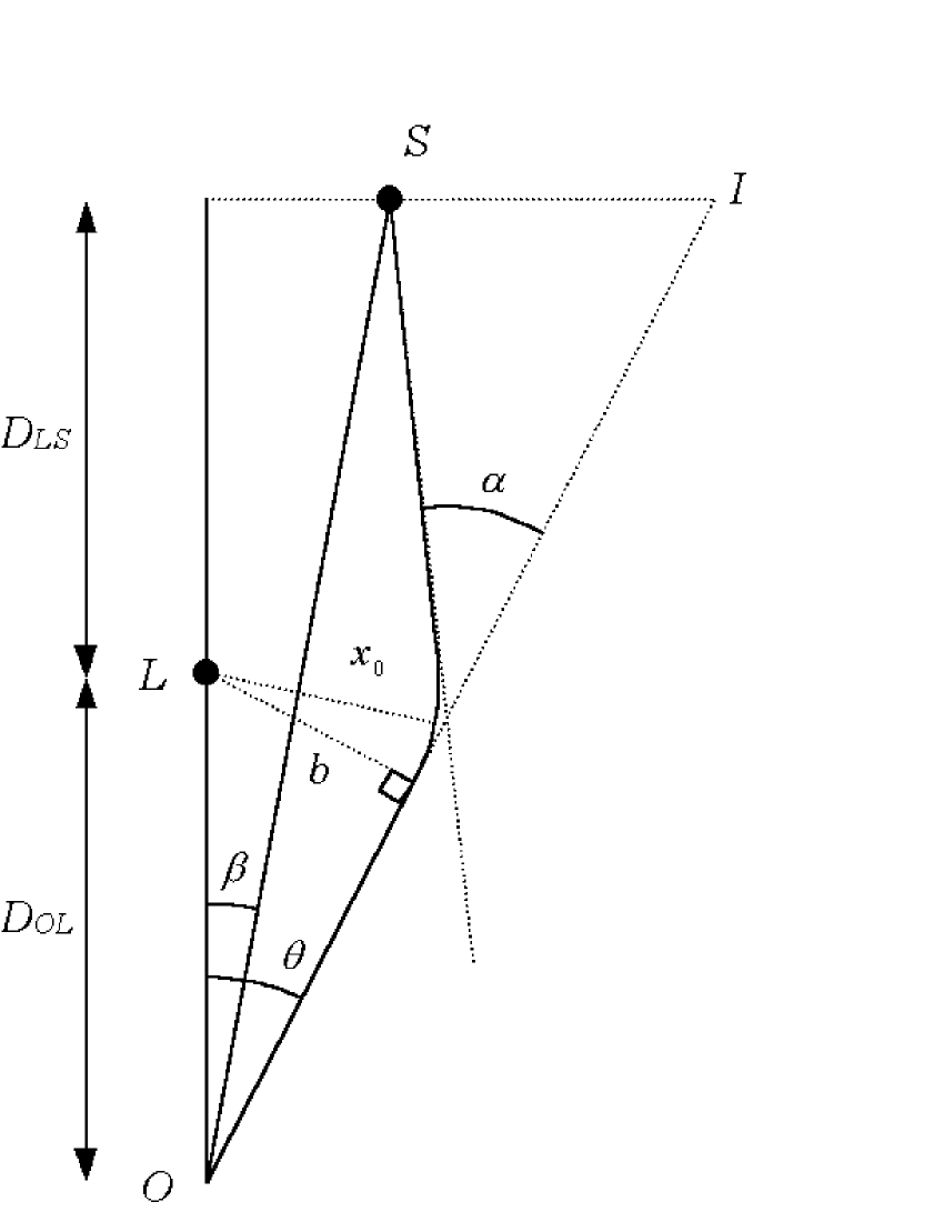
FIG. 1.: Geometrical configuration of gravitational lensing. Light rays emitted by the source $S$ are deflected by the lens $L$ and reach the observer $O$ with an angle $\theta$, instead of $\beta$. The total deflection angle is $\alpha$. $x_{0}$ is the closest approach distance and $b$ is the impact parameter. $D_{OL}$ is the distance between the lens and the observer. $D_{LS}$ is the distance between the lens and the projection of the source on the optical axis $OL$. $D_{OS}=D_{OL}+D_{LS}$.

FIG. 2.: Deflection angle as a function of the closest approach distance.

FIG. 3.: Ratio of the exact deflection angle (3) and the approximate one (10) as functions of the closest approach distance.

REFERENCES

- [1] Schneider P., Ehlers J., Falco E.E.,1992, Gravitational lenses, Springer-Verlag, Berlin.
- [2] Will C.M., 1993, Theory and Experiments in Graviational Physics, Cambridge Univ. Press, Cambridge.
- [3] Viergutz S.U., 1993, A&A 272, 355
- [4] Bardeen J.M., 1973, Black Holes, ed. C. de Witt & B.S. de Witt, NY, Gordon & Breach, 215
- [5] Falcke H., Melia F., Agol E., 1999, astro-ph/9912263
- [6] Virbhadra K.S., Ellis G.F.R., 1999, astro-ph/9904193
- [7] Frittelli S., Kling T.P. & Newman E.T., 2000, Phys. Rev. D 61, 064021
- [8] Weinberg S., 1972, Gravitation and cosmology: principles and applications of the general theory of relativity, John Wiely & Sons, NY
- [9] Richstone D., Ajhar E:A:, Bender R. et al. 1998, Nat 395, A14
- [10] Hirabayashi H., 1990, Observatories in earth orbit and beyond(A93-23401 07-89), 263
- [11] Ulvestad J.S., 1999, “Goals of the ARISE Space VLBI Mission”, New Astronomy Reviews, Proceedings of the 4th EVN/JIVE Symposium