Hamiltonian structure of 2+1 dimensional gravity

Abstract

A summary is given of some results and perspectives of the hamiltonian ADM approach to $2+1$ dimensional gravity. After recalling the classical results for closed universes in absence of matter we go over the the case in which matter is present in the form of point spinless particles. Here the maximally slicing gauge proves most effective by relating $2+1$ dimensional gravity to the Riemann- Hilbert problem. It is possible to solve the gravitational field in terms of the particle degrees of freedom thus reaching a reduced dynamics which involves only the particle positions and momenta. Such a dynamics is proven to be hamiltonian and the hamiltonian is given by the boundary term in the gravitational action. As an illustration the two body hamiltonian is used to provide the canonical quantization of the two particle system.

1 Introduction

The past fifteen years have witnessed a remarkable interest in gravity in 2+1 dimensions DJH both at the classical and quantum level.

In this paper we shall summarize some old results and some recent developments with regard to the hamiltonian formulation of the theory. We shall insist on the conceptual side; the technical details can be found in the published papers and reports.

2 2+1 dimensional gravity in absence of matter

In absence of matter the only degrees of freedom are given by the moduli of the space sections; thus the open universe case and the case of the sphere topology are trivial.

In absence of boundaries the action of the gravitational field reduces to the Einstein- Hilbert term which can be put in hamiltonian form as

$$S_{H}=\int dt\int_{\Sigma_{t}}d^{D}x\left[\pi^{ij}\dot{g}_{ij}-N^{i}H_{i}-NH\right]$$ (1)

where we used the standard ADM metric ADM

$$ds^{2}=-N^{2}dt^{2}+2g_{z\bar{z}}(dz+N^{z}dt)(d\bar{z}+N^{\bar{z}}dt).$$ (2)

The choice of the gauge is of crucial importance in dealing with the problem. The well known York gauge in which the time slices are provided by the $D$ (in our case $D=2$) dimensional surfaces with $K={\rm const.}$, being $K$ the trace of the intrinsic curvature tensor is particularly powerful as this gauge decouples the solution of the diffeomorphism constraint from that of the hamiltonian constraint. Exploiting this feature it is possible moncrief ; hosoya to solve the diffeomorphism constraint and to provide the hamiltonian on the reduced phase space given by the moduli and their conjugate momenta. The number of moduli are $6g-6$ for genus $g$ larger than $1$ and $2$ for the torus topology. The explicit computation of the hamiltonian can be performed only in the simplest case of torus topology. It is given by

$$H=\sqrt{\tau^{2}_{2}(p_{1}^{2}+p_{2}^{2})}.$$ (3)

Quantization proceeds hosoya2 ; carlip by replacing the canonical variables with operators according to the correspondence principle. The ordering problem always subsists; the most natural ordering translates the classical hamiltonian into the square root of the Maass laplacian maass giving rise to the Schroedinger equation

$$i\frac{\partial\psi(x,y,t)}{\partial t}=\sqrt{-y^{2}(\partial_{x}^{2}+\partial_{y}^{2})}~{}\psi(x,y,t).$$ (4)

The Maass laplacian has been widely investigated by mathematicians fay ; terras ; puzio . The classical as well the quantum hamiltonians are invariant under modular transformations which in the case of the torus is given by the group $SL(2,Z)$ and thus the solutions should be invariant under such modular transformations. The eigenvalue problem under this condition is not trivial and the spectrum well studied fay ; terras ; puzio . Such an approach gives a complete quantum treatment of universes without matter with torus topology in the York gauge.

3 2+1 dimensional gravity coupled to particles

We come now to the more difficult and realistic case of gravity coupled to particles. It describes also a situation of 3+1 dimensional gravity, i.e. the interaction of parallel cosmic strings.

One starts from the action of the gravitational field coupled to a finite number of spinless point particles. The inclusion of spin to point particles is not a trivial issue as it gives rise to closed time like curves.

We must add to the action (1) the particle action

$$S_{m}=\int\!dt\sum_{n}\Big{(}P_{ni}\,\dot{q}_{n}^{i}+N^{i}(q_{n})P_{ni}-N(q_{n})\sqrt{P_{ni}P_{nj}g^{ij}(q_{n})+m_{n}^{2}}\Big{)}$$ (5)

and for open universes we must also add boundary terms; we shall adopt here the so called Trace-$K$ form completed of the terms which lye on two sub-manifolds of dimension $D-1$, being $D+1$ the dimension of space- time hawkinghunter ; brownyork . In hamiltonian form it reduces to

$$S_{B}=-\int dtH_{B}$$ (6)

with

$$-H_{B}=2\int_{B_{t}}d^{(D-1)}x\,\sqrt{\sigma_{Bt}}N\left(K_{B_{t}}+\frac{\eta}{\cosh\eta}{\cal D}_{\alpha}v^{\alpha}\right)$$

$$~{}~{}~{}~{}~{}~{}~{}~{}~{}~{}~{}~{}~{}~{}~{}-2\int_{B_{t}}d^{(D-1)}x\,r_{\alpha}\pi^{\alpha\beta}_{(\sigma_{Bt})}N_{\beta}.$$ (7)

The really important term turns out to be the first i.e. $\sqrt{\sigma_{Bt}}NK_{B_{t}}$ where $K_{B_{t}}$ is the extrinsic curvature of the $D-1$ dimensional boundary (in our case one- dimensional) of the time slices as a sub-manifold embedded in the $D$ dimensional time slices and $d^{(D-1)}x\sqrt{\sigma_{Bt}}$ is the volume form induced by the space metric on the $D-1$ dimensional boundary.

We recall that the action $S_{H}+S_{B}+S_{m}$ is so constructed as to provide the correct equations of motion (i.e. Einstein’s equations) when one computes a stationary point of the action by keeping the values of the metric fixed on the boundary. Such a procedure is equivalent wald to the weaker requirement of keeping fixed the intrinsic metric of the boundary.

One could in principle adopt also here the York slicing. However the equations for the diffeomorphism and hamiltonian constraints are not at all trivial. In particular the hamiltonian constraint gives rise to an equation more complex than the inhomogeneous sine-Gordon equation. Progress has been achieved by the introduction of the instantaneous York gauge BCV ; welling ; MS1 ; MS2 ; CMS , or maximally slicing gauge. This is defined by all time slices having $K=0$. Simple application of the Gauss- Bonnet theorem shows that such a gauge can be applied only to open universes, or universes with the topology of the sphere welling ; MS1 . In addition a closer inspection shows that for the sphere topology it can describe only the simple stationary case MS2 . Thus application of the $K=0$ gauge is practically restricted to open universes, but here it proves very powerful. The technical reason is the immediate solution of the diffeomorphism constraint given by

$$\pi^{\bar{z}}_{~{}z}=-\frac{1}{2\pi}\sum_{n}\frac{P_{n}}{z-z_{n}}\equiv-2\frac{\prod_{B}(z-z_{B})}{{\cal P}(z)},$$ (8)

where $z_{n}$ and $P_{n}$ are the complex positions and canonical momenta of the particles, and the reduction of the hamiltonian constraint to an inhomogeneous Liouville equation, given by

$$2\Delta\tilde{\sigma}=-e^{-2\tilde{\sigma}}-4\pi\sum_{n}\delta^{2}(z-z_{n})(\mu_{n}-1)-4\pi\sum_{B}\delta^{2}(z-z_{B}),$$ (9)

to which powerful mathematical methods apply kra . Here $\tilde{\sigma}$ is defined by

$$e^{2\sigma}=2\pi^{\bar{z}}_{~{}z}\pi^{z}_{~{}\bar{z}}e^{2\tilde{\sigma}},$$ (10)

and is related to the space metric by $g_{ij}=\delta_{ij}e^{2\sigma}$. In the above equation the sources are given by the particle and in addition by the zeros of eq.(8) here denoted by $z_{B}$. These are the points where the extrinsic curvature tensor vanishes, and through the Gauss-Codazzi relation also the intrinsic curvature scalar of the time slice vanishes. It is interesting that such $z_{B}$ coincide with the positions of the accessory singularities which will appear in the uniformization problem. These accessory parameters summarize all the gravitational interaction. An interesting restriction occurs on the conjugate momenta i.e. $\sum_{n}P_{n}=0$ Des85 . In absence of such a restriction no solution exists to eq.(9) with $\exp({2\sigma})$ behaving at infinity with $\exp({2\sigma})\approx s^{2}(z\bar{z})^{-\mu}$ which describes a space geometry asymptotic to a cone. This can be easily seen by applying the divergence theorem to the analogous of eq.(9) for $\sigma$. The same reasoning excludes the addition of an holomorphic term to the $\pi^{\bar{z}}_{~{}z}$ given by eq.(8)

The solution of the inhomogeneous Liouville equation (9) can be understood as a variant of the Riemann- Hilbert problem and is reduced to a linear fuchsian differential equation bolibrukh . By taking the ratio of two solutions of such equation one can build the function $f(z)$ which maps the metric of the Poincaré pseudo-sphere into the conformal factor which solves (9) according to the formula kra

$$e^{-2\tilde{\sigma}}=\frac{8f^{\prime}(z)\bar{f}^{\prime}(\bar{z})}{(1-f(z)\bar{f}(\bar{z}))^{2}}=\frac{{\rm const}}{(\bar{y}_{2}(\bar{z})y_{2}(z)-\bar{y}_{1}(\bar{z})y_{1}(z))^{2}};~{}f(z)=\frac{y_{1}(z)}{y_{2}(z)}$$ (11)

It is a variant of the Riemann-Hilbert problem as we are not given directly with the monodromies but with the following information on them: all monodromies belong to the $SU(1,1)$ group, otherwise the conformal factor (11) is not single valued and as such cannot solve the Liouville equation eq.(9); in addition we are given with the conjugation classes of the monodromies around the particles (the particle masses), the conjugation class of the monodromy at infinity (the total energy) and the positions of the auxiliary singularities $z_{B}$, which are equivalent to the knowledge of the particle momenta $P_{n}$ up to a multiplicative factor. Due to the relation $\sum_{n}P_{n}=0$ the number of auxiliary singularities is ${\cal N}-2$.

In order to count the physical degrees of freedom in addition to the particle positions, we must keep in mind that for ${\cal N}$ particles we have ${\cal N}$ $SU(1,1)$ monodromies to which we have to subtract a $SU(1,1)$ conjugation thus reaching $3{\cal N}-3$ real degrees of freedom. These are equivalent to giving the ${\cal N}$ particle masses $\mu_{i}$, the total energy $\mu$ and the complex positions $z_{B}$ of the ${\cal N}-2$ auxiliary singularities i.e. $3{\cal N}-3={\cal N}+1+2({\cal N}-2)$. The linear residues $\beta_{B}$ of the auxiliary singularities are fixed by the solution of the Riemann- Hilbert problem while the linear residues $\beta_{i}$ at the particle singularities are computed from the ${\cal N}-2$ no logarithm condition at the auxiliary singularities and the first and second Fuchs conditions on the residues of the fuchsian differential equation.

The conformal factor $\tilde{\sigma}$ is the key quantity in all the subsequent developments. In fact a secondary constraint following from the primary gauge constraint $K=0$ is

$$\Delta N=e^{-2\tilde{\sigma}}N$$ (12)

and such $N$ can be computed from the knowledge of $\tilde{\sigma}$. The reason is that the solution of the inhomogeneous Liouville equation (9) contains a free parameter $\mu$ which is related to the behavior at infinity of the conformal factor i.e. $\exp(2\sigma)=s^{2}(z\bar{z})^{-\mu}$. As the sources do not depend on $\mu$ a solution of eq.(12) is given by

$$N=\frac{\partial(-2\tilde{\sigma})}{\partial M}$$ (13)

and one easily proves such a solution to be unique. The other secondary constraint on $N^{z}$ is

$$\partial_{\bar{z}}N^{z}=-\pi^{z}_{~{}\bar{z}}~{}e^{-2\sigma}N$$ (14)

solved by

$$N^{z}=-\frac{2}{\pi^{\bar{z}}_{\ z}(z)}\partial_{z}N+g(z).$$ (15)

Here $g(z)$ is a meromorphic function whose role is to cancel the poles occurring in the first member on the r.h.s. due to the zeros of $\pi^{\bar{z}}_{\ z}$. The expression of $g(z)$ in $N^{z}$ is MS1

$$g(z)=\sum_{B}\frac{\partial\beta_{B}}{\partial M}\frac{1}{z-z_{B}}\frac{{\cal P}(z_{B})}{\prod_{C\neq B}(z_{B}-z_{C})}+p_{1}(z).$$ (16)

$p_{1}(z)$ is a first order polynomial related to the motion of the frame at infinity, more properly henneaux ; ashtekar to the gauge transformation of translations, rotations and dilatations which leave invariant the conformal structure of the space metric and leave fixed the point at infinity.

In conclusion the metric is obtained in a straightforward way from $\tilde{\sigma}$. The particle equations of motion are extracted from the variation of the action with respect to particle momenta and coordinates and take the form MS1

$$\dot{z}_{n}=-N^{z}(z_{n})=-g(z_{n})=$$

$$-\sum_{B}\frac{\partial\beta_{B}}{\partial M}\frac{1}{z_{n}-z_{B}}\frac{{\cal P}(z_{B})}{\prod_{C\neq B}(z_{B}-z_{C})}-p_{1}(z_{n})$$ (17)

$$\dot{P}_{nz}=4\pi\frac{\partial\beta_{n}}{\partial M}+P_{nz}~{}g^{\prime}(z_{n})=$$

$$=4\pi\frac{\partial\beta_{n}}{\partial M}-P_{nz}\sum_{B}\frac{\partial\beta_{B}}{\partial M}\frac{{\cal P}(z_{B})}{(z_{n}-z_{B})^{2}\prod_{C\neq B}(z_{B}-z_{C})}+P_{nz}~{}p^{\prime}_{1}(z_{n}).$$ (18)

As already mentioned the linear polynomial $p_{1}(z)$ is related to the choice of the frame at infinity. The choice of the frame which does not rotate and dilatate at infinity imposes that $N^{z}$ contains no linear term and thus fixes

$$p_{1}(z)=c_{0}-~{}\frac{1}{\sum_{n}P_{n}z_{n}}~{}z.$$ (19)

An interesting generalized conservation law which holds for any number of particles can be derived MS1 from eqs.(17,18)

$$\sum_{n}P_{n}z_{n}=(1-\mu)(t-t_{0})-iL.$$ (20)

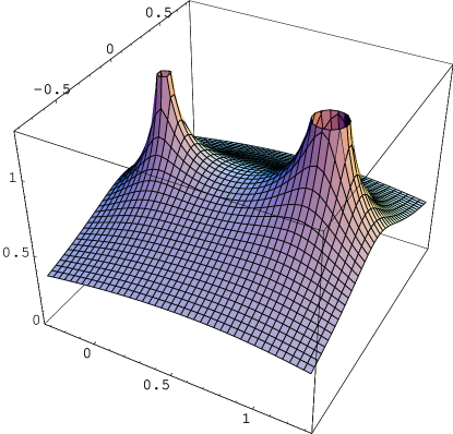
Figure 1: Conformal factor for the classical two body problem

For the two body problem we have no auxiliary singularity and the fuchsian differential equation underlying the solution of eq.(9) is the hypergeometric equation. The conformal factor can be easily expressed in term of hypergeometric functions, thus giving a complete information on the metric. Equations (17,18) take a very simple form in the two body case due to the absence of apparent singularities. It is interesting that the equations of motion can be explicitly written just by looking at the local properties of the fuchsian differential equation which underlies the solution of eq.(9). We obtain going over to the relative coordinates $z^{\prime}_{2}=z_{2}-z_{1}$ and $P^{\prime}=P_{2}=-P_{1}$

$$\dot{z}^{\prime}_{2}=\frac{1}{P^{\prime}_{z}};~{}~{}~{}~{}\dot{P}^{\prime}_{z}=-\frac{\mu}{z^{\prime}_{2}}.$$ (21)

being $4\pi\mu=M$ the total mass (energy) of the system. One immediately realizes that such equations of motion (and their complex conjugate) are generated by the hamiltonian $H=h+\bar{h}$ with $h=\ln(P^{\prime}{z^{\prime}}_{2}^{\mu})$ where $h$ and $\bar{h}$ are constants of motion. Taking the ratio of $P^{\prime}{z^{\prime}}_{2}^{\mu}=\exp(h)={\rm const.}$ with eq.(20) we obtain the solution for the particle motion

$$z={\rm const}[(1-\mu)(t-t_{0})-iL]^{\frac{1}{1-\mu}}.$$ (22)

without the need to solve the system (21). Thus the two body problem is integrable. Solution (22) was first found in BCV . The fact that only the total energy $M=4\pi\mu$ intervenes in eq.(22) constitutes a proof of a conjecture by ’t Hooft hooft3 about the independence of the solution of the two body problem of the masses of the constituent particles.

In Fig.1 we report the conformal factor for the two body problem for $\mu_{1}=0.1$, $\mu_{2}=0.2$ and $\mu=0.5$

4 The N body problem

In the coordinate frame in which the polynomial $p_{1}$ vanishes the equations of motion in the relative coordinates $z^{\prime}_{n}=z_{n}-z_{1}$, $P^{\prime}_{n}=P_{n}$ for $n=2\dots{\cal N}$ take the form CMS

$$\dot{z}^{\prime}_{n}=-\sum_{B}\frac{\partial\beta_{B}}{\partial\mu}\frac{\partial z^{\prime}_{B}}{\partial P^{\prime}_{n}}~{}~{}~{}~{}~{}~{}~{}~{}n=2,\dots{\cal N}$$ (23)

and

$$\dot{P}^{\prime}_{n}=\frac{\partial\beta_{n}}{\partial\mu}+\sum_{B}\frac{\partial\beta_{B}}{\partial\mu}\frac{\partial z^{\prime}_{B}}{\partial z^{\prime}_{n}}~{}~{}~{}~{}~{}~{}~{}~{}n=2,\dots{\cal N}.$$ (24)

These equations are canonically related to the ones with $p_{1}\neq 0$ and thus is sufficient to examine them. The problem is now to show that such system is of hamiltonian nature; such a result is expected as we obtained the above equations by reduction of a hamiltonian system. Despite that, it is of interest to have a direct proof of it and an expression of the hamiltonian.

In the simpler case of three body, where we have a single auxiliary singularity, one immediately sees that the hamiltonian has to be of the form

$$H(z^{\prime}_{2},z^{\prime}_{3},P^{\prime}_{2},P^{\prime}_{3})=-\int_{z_{0}}^{z^{\prime}_{A}}\frac{\partial\beta_{A}}{\partial\mu}(z^{\prime}_{2},z^{\prime}_{3},z^{\prime\prime}_{A})~{}dz^{\prime\prime}_{A}+f(z^{\prime}_{2},z^{\prime}_{3})+~{}c.c.$$ (25)

$H$ generates the equations for $\dot{z}^{\prime}_{n}$ for any $f(z^{\prime}_{2},z^{\prime}_{3})$; the function $f$ has to be determined by requiring that the same $H$ generates also the equations for $\dot{P}^{\prime}_{n}$. This imposes some integrability conditions on the function $\beta_{A}$; such conditions are satisfied due to the validity of the Garnier equations which give a constraint on the evolution of the auxiliary parameters under isomonodromic deformations yoshida ; okamoto . The fact that our deformations are isomonodromic is a consequence of the constancy in $2+1$ dimensional gravity of the monodromies around the particle world lines. It is of interest that such equations can be derived directly form the ADM formalism as equations of motion MS1 .

The problem with four or more particle, when we are in presence of two or more auxiliary singularities is more difficult and it related to an interesting conjecture due to Polyakov ZT1 about the auxiliary parameters of the $SU(1,1)$ Riemann-Hilbert problem. Such a conjecture states that the regularized Liouville action takh

$$S_{\epsilon}[\phi]=\frac{i}{2}\int_{X_{\epsilon}}(\partial_{z}\phi\partial_{\bar{z}}\phi+\frac{e^{\phi}}{2})dz\wedge d\bar{z}-\frac{i}{2}\sum_{n}(1-\mu_{n})\oint_{n}\phi(\frac{d\bar{z}}{\bar{z}-\bar{z}_{n}}-\frac{dz}{z-z_{n}})$$

$$+\frac{i}{2}\sum_{B}\oint_{B}\phi(\frac{d\bar{z}}{\bar{z}-\bar{z}_{B}}-\frac{dz}{z-z_{B}})-\frac{i}{2}(\mu-2)\oint_{\infty}\phi(\frac{d\bar{z}}{\bar{z}}-\frac{dz}{z})$$

$$-\pi\sum_{n}(1-\mu_{n})^{2}\ln\epsilon^{2}-\pi\sum_{B}\ln\epsilon^{2}-\pi(\mu-2)^{2}\ln\epsilon^{2}$$ (26)

is the generator of the linear residues $\beta_{i}$, $\beta_{B}$ in the fuchsian differential equation whose solutions provide the mapping function which solve the inhomogeneous Liouville equation, i.e.

$$-\frac{1}{2\pi}dS_{\epsilon}=\sum_{n}\beta_{n}dz_{n}+\sum_{B}\beta_{B}dz_{B}+~{}c.c.$$ (27)

Such a conjecture has been proven by Zograf and Takhtajan ZT1 for the case of parabolic singularities and elliptic singularities of finite order. In the context of 2+1 dimensional gravity with generic masses one should need the validity of such a conjecture for generic elliptic singularities. The relevance of such a conjecture is that it gives a new meaning to the auxiliary parameters; moreover it is a straightforward consequence of eq.(27) that, apart from a constant

$$H=\frac{1}{2\pi}\frac{\partial S_{\epsilon}}{\partial\mu}\$$ (28)

as can be seen by computing $\frac{\partial H}{\partial P^{\prime}_{n}}$, $\frac{\partial H}{\partial z^{\prime}_{n}}$ and comparing with eqs.(23,24). We recall that in the non rotating frame the hamiltonian contains an additional contribution, as already observed in sect. 3. Its complete form in that frame is indeed given by CMS

$$H=\ln\left[(\sum_{n}P_{n}z_{n})(\sum_{n}\bar{P}_{n}\bar{z}_{n})\right]+\frac{1}{2\pi}\frac{\partial S_{\epsilon}}{\partial\mu}.$$ (29)

Note that this hamiltonian, being time-independent, provides a further conservation law in the ${\cal N}-$particle problem.

The hamiltonian $H$ has been constructed from the equations of motion. On the other hand it should be possible to derive directly the reduced hamiltonian starting from the action after replacing into it the solution of the constraints. As in our gauge $\pi^{ij}\dot{g}_{ij}=0$, the action reduces to

$$S=\int dt(\sum_{n}P_{ni}\,\dot{q}_{n}^{i}-H_{B})$$ (30)

with $H_{B}$ given by eq.(7). The last term in $H_{B}$ contributes to a constant while the term proportional to $\eta/\cosh\eta$ goes to zero at large distances. Thus we are left only with the term proportional to $K_{Bt}$ which for large $r_{0}$ can be computed to give CMS

$$H_{B}=-r_{0}\ln r_{0}^{2}(\frac{1}{r_{0}}+\partial_{r}\sigma)=(\mu-1)\ln r_{0}^{2}.$$ (31)

We recall now that the equations of motion are obtained from the action by keeping the values of the fields fixed at the boundary, or equivalently wald by keeping fixed the intrinsic metric of the boundary. In our case the variations should be performed keeping fixed the fields $N$, $N^{a}$, and $\sigma$ at the boundary. We shall perform the computation for the boundary given by a circle of radius $r_{0}$ for a very large value of $r_{0}$. The asymptotic form of the conformal factor $2\sigma$ is

$$2\sigma=\ln s^{2}-\mu\ln r_{0}^{2}.$$ (32)

If we change the particle positions and momenta, $s^{2}$ varies and in order to keep the value of $\sigma$ fixed at the boundary we must vary $\mu$ as follows

$$0=-\delta\mu\ln r_{0}^{2}+\delta\ln s^{2}$$ (33)

i.e. for large $r_{0}$

$$\delta\mu\approx\frac{1}{\ln r_{0}^{2}}\delta\ln s^{2}.$$ (34)

Substituting into eq.(31) we have

$$H_{B}=\ln s^{2}+{\rm const.}$$ (35)

i.e. the hamiltonian is given by the logarithm of the coefficient of the asymptotic expansion of the conformal factor at large distances.

We want now to relate the result eq.(35) to the results obtained directly from the equations of motion.

Let us consider the value of the action $S_{\epsilon}$ on the solution of the Liouville equation and let us compute its derivative with respect to $\mu$. As we are varying around a stationary point the only contribution is provided by the terms in eq.(26) which depend explicitly on $\mu$ i.e.

$$\frac{\partial S_{\epsilon}}{\partial\mu}=-\frac{i}{2}\oint_{\infty}\phi(\frac{d\bar{z}}{\bar{z}}-\frac{dz}{z})-2\pi(\mu-2)\ln\epsilon^{2}$$ (36)

and as $\phi\equiv-2\tilde{\sigma}$ at infinity behaves like

$$\phi\approx(\mu-2)\ln z\bar{z}+\ln\left[(\sum_{n}P_{n}z_{n})(\sum_{n}\bar{P}_{n}\bar{z}_{n})\right]-\ln s^{2}+{\rm const}$$ (37)

we have

$$\frac{1}{2\pi}\frac{\partial S_{\epsilon}}{\partial\mu}=-\ln\left[(\sum_{n}P_{n}z_{n})(\sum_{n}\bar{P}_{n}\bar{z}_{n})\right]+\ln s^{2}+{\rm const}$$ (38)

which substituted in eq.(35) gives

$$H=\ln\left[(\sum_{n}P_{n}z_{n})(\sum_{n}\bar{P}_{n}\bar{z}_{n})\right]+\frac{1}{2\pi}\frac{\partial S_{\epsilon}}{\partial\mu}+{\rm const}$$ (39)

in agreement with the result (29) obtained through Polyakov’s conjecture.

It is remarkable that the same hamiltonian is obtained independently from the boundary term of the $2+1$ gravitational action and from the equations of motion in conjunction with Polyakov conjecture. This lends support to the validity of Polyakov’s conjecture in the general elliptic case or at least to a weak form of it, obtained by taking the derivative of eq.(27) with respect to $\mu$.

5 Quantization: the two particle case

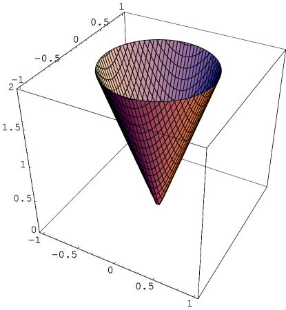
Figure 2: Cone metric equivalent to the classical metric of Fig.1, intervening in the quantum two body problem

Several quantization scheme have been put forward in the context of $2+1$ dimensional gravity (see e.g. hosoya2 ; carlip ; hooft ; wael ; nelsonregge ; matschull ). Here we shall examine the canonical quantization which flows directly from the hamiltonian ADM formalism ADM . We recall that the classical two particle hamiltonian in the reference system which does not rotate at infinity is given by

$$H=\ln(Pz\bar{P}\bar{z})+(\mu-1)\ln(z\bar{z})=\ln(Pz^{\mu})+\ln(\bar{P}\bar{z}^{\mu})=h+\bar{h}$$ (40)

with $P=P^{\prime}_{2}$ and $z=z^{\prime}_{2}$. $H$ can be rewritten in cartesian coordinates as

$$H=\ln((x^{2}+y^{2})^{\mu}((P_{x})^{2}+(P_{y})^{2})).$$ (41)

Keeping in mind that with our definitions $P$ is the momentum multiplied by $16\pi G_{N}/c^{3}$, applying the correspondence principle we have

$$[x,P_{x}]=[y,P_{y}]=il_{P}$$ (42)

where $l_{P}=16\pi G_{n}\hbar/c^{3}$, all other commutators equal to zero. $H$ is converted into the operator

$$\ln[-(x^{2}+y^{2})^{\mu}\Delta]+~{}{\rm constant}.$$ (43)

The argument of the logarithm is the Laplace-Beltrami $\Delta_{LB}$ operator on the metric $ds^{2}=(x^{2}+y^{2})^{-\mu}(dx^{2}+dy^{2})$. We note that in the quantum problem only the simple metric of a cone (see Fig.2) intervenes and not the classical metric of Fig.1. The angular deficit of the cone again in given by the total energy thus proving ’t Hooft conjecture hooft3 at the quantum level. Following an argument similar to the one presented in sorkin one easily proves that if we start from the domain of $\Delta_{LB}$ given by the infinite differentiable functions of compact support $C^{\infty}_{0}$ which can also include the origin, then $\Delta_{LB}$ has a unique self-adjoint extension in the Hilbert space of functions square integrable on the metric $ds^{2}=(x^{2}+y^{2})^{-\mu}(dx^{2}+dy^{2})$ CMS and as a result since $\Delta_{LB}$ is a positive operator, $\ln(\Delta_{LB})$ is also self-adjoint.

Deser and Jackiw deserjackiw considered the quantum scattering of a test particle on a cone both at the relativistic and non relativistic level. Most of the techniques developed there can be transferred here. The main difference is the following; instead of the hamiltonian $(x^{2}+y^{2})^{\mu}(p_{x}^{2}+p_{x}^{2})$ which appears in their non relativistic treatment, we have now the hamiltonian $\ln[(x^{2}+y^{2})^{\mu}(p_{x}^{2}+p_{y}^{2})]$. The partial wave eigenvalue differential equation

$$(r^{2})^{\mu}[-\frac{1}{r}\frac{\partial}{\partial r}r\frac{\partial}{\partial r}+\frac{n^{2}}{r^{2}}]\phi_{n}(r)=k^{2}\phi_{n}(r)$$ (44)

with $\mu=1-\alpha$ is solved by

$$\phi_{n}(r)=J_{\frac{|n|}{\alpha}}(\frac{k}{\alpha}r^{\alpha})$$ (45)

and out of them one can compute the quantum Green function which in our case can be expressed in terms of hypergeometric functions CMS . The ordering problem always subsists; the one adopted in (43) is the most natural. In the ${\cal N}$-body problem due to the complexity of the hamiltonian we expect the ordering problem to be more acute. Power expansions in some small parameter like the total kinetic energy or the particle masses may give useful indications.

References

- (1) A. Staruszkiewicz, Acta Phys. Polonica 24 (1963) 734; S. Deser, R. Jackiw and G. ’t Hooft, Ann. Phys. (NY) 152 (1984) 220; S. Deser and R. Jackiw, Ann. Phys. 153 (1984) 405
- (2) R. Arnowitt, S. Deser and C.W. Misner, in “Gravitation: an introduction to current research” Edited by L. Witten, John Wiley & Sons New York, London 1962
- (3) V. Moncrief, J. Math. Phys. 30 (1989) 2907
- (4) A. Hosoya and K. Nakao, Class. Quantum Grav. 7 (1990) 163
- (5) A. Hosoya and K. Nakao, Progr. Theor. Phys. 84 (1990) 739
- (6) S. Carlip, Phys. Rev. D42 (1990) 2647; Phys. Rev. D45 (1992) 3584
- (7) H. Maass, Lectures on modular functions of one complex variable, Tata Institute, Bombay (1964)
- (8) J.D. Fay, J. Reine Angew. Math. 293 (1977) 143
- (9) A. Terras, Harmonic analysis on symmetric spaces and applications, Springer- Verlag, Berlin, (1985)
- (10) R. Puzio, Classical and Quantum Gravity 11 (1994) 609
- (11) S.W. Hawking and C. J. Hunter, Class. Quantum Grav. 13 (1996) 2735; G. Hayward, Phys. Rev. D 47 (1993) 3275
- (12) J. D. Brown, S. R. Lau, J. W. York gr-qc/ 0010024 and references therein.
- (13) R. M. Wald, “General Relativity”, The University of Chicago Press, Chicago and London (1984)
- (14) A. Bellini, M. Ciafaloni, P. Valtancoli, Physics Lett. B 357 (1995) 532; Nucl. Phys. B 462 (1996) 453
- (15) M. Welling, Class. Quantum Grav. 13 (1996) 653; Nucl. Phys. B 515 (1998) 436
- (16) P. Menotti, D. Seminara, Ann. Phys. 279 (2000) 282
- (17) P. Menotti, D. Seminara, Nucl. Phys. (Proc. Suppl.) 88 (2000) 132.
- (18) L. Cantini, P. Menotti, D. Seminara, hep-th/0011070 to appear in “Classical and quantum gravity”
- (19) J. Liouville J. Math. Pures Appl. 18 (1853) 71; H. Poincaré, J. Math. Pures Appl. 5 ser.2 (1898) 157; P. Ginsparg and G. Moore, hep-th/9304011; L. Takhtajan, “Topics in quantum geometry of Riemann surfaces: two dimensional quantum gravity”, Como Quantum Groups (1994) 541, hep-th/9409088; I. Kra, “Automorphic forms and Kleinian groups” Benjamin, Reading Mass., 1972.
- (20) S. Deser, Class. Quantum Grav. 2 (1985) 489.
- (21) See e.g. A.A. Bolibrukh, Uspekhi Mat. Nauk 45:2 (1990) 3
- (22) M. Henneaux, Phys. Rev. D 29 (1984) 2767
- (23) A. Ashtekar, M. Varadarajan, Phys. Rev. D 50 (1994) 4944
- (24) G. ’t Hooft, Comm. Math. Phys. 117 (1988) 685
- (25) M. Yoshida, “Fuchsian differential equations”, Fried. Vieweg & Sohn, Braunschweig (1987)
- (26) K. Okamoto, J. Fac. Sci. Tokio Univ. 33 (1986)
- (27) P. G. Zograf, L. A. Tahktajan, Math. USSR Sbornik 60 (1988) 143
- (28) L. A. Takhtajan, Mod. Phys. Lett. A11 (1996) 93
- (29) G. ’t Hooft, Class. Quantum Grav. 9 (1992) 1335; Class. Quantum Grav. 10 (1993) 1023, Class. Quantum Grav. 10 (1993) 1653; Class. Quantum Grav. 13 (1996) 1023
- (30) H. Waelbroeck, Class. Quantum Grav. 7 (1990) 751; Phys. Rev. D50 (1994) 4982
- (31) J. Nelson, T. Regge, Phys. Lett. B273 (1991) 213
- (32) M. Welling, Class. Quant. Grav. 14 (1997) 3313; H-J. Matschull and M. Welling, Class. Quantum Grav. 15 (1998) 2981
- (33) M. Bourdeau, S. D. Sorkin, Phys. Rev. D 45 (1992) 687
- (34) S. Deser, R. Jackiw, Comm. Math. Phys. 118 (1988) 495