On the role of $\Lambda$-term in the evolution of Bianchi-I cosmological model with nonlinear spinor field

Abstract

Self-consistent solutions to nonlinear spinor field equations in General Relativity are studied for the case of Bianchi type-I space-time. It has been shown that introduction of $\Lambda$-term in the Lagrangian generates oscillations of the Bianchi type-I model.

Key words: Nonlinear spinor field (NLSF), Bianch type -I model (B-I), $\Lambda$ term PACS 98.80.C Cosmology

1 Introduction

The quantum field theory in curved space-time has been a matter of great interest in recent years because of its applications to cosmology and astrophysics. The evidence of existence of strong gravitational fields in our Universe led to the study of the quantum effects of material fields in external classical gravitational field. After the appearance of Parker’s paper on scalar fields [1] and spin-$\frac{1}{2}$ fields, [2] several authors have studied this subject. Although the Universe seems homogenous and isotropic at present, there are no observational data guarantying the isotropy in the era prior to the recombination. In fact, there are theoretical arguments that sustain the existence of an anisotropic phase that approaches an isotropic one  [3]. Interest in studying Klein-Gordon and Dirac equations in anisotropic models has increased since Hu and Parker [4] have shown that the creation of scalar particles in anisotropic backgrounds can dissipate the anisotropy as the Universe expands.

A Bianchi type-I (B-I) Universe, being the straightforward generalization of the flat Robertson-Walker (RW) Universe, is one of the simplest models of an anisotropic Universe that describes a homogenous and spatially flat Universe. Unlike the RW Universe which has the same scale factor for each of the three spatial directions, a B-I Universe has a different scale factor in each direction, thereby introducing an anisotropy to the system. It moreover has the agreeable property that near the singularity it behaves like a Kasner Universe, even in the presence of matter, and consequently falls within the general analysis of the singularity given by Belinskii et al [5]. Also in a Universe filled with matter for $p\,=\,\gamma\,\varepsilon,\quad\gamma<1$, it has been shown that any initial anisotropy in a B-I Universe quickly dies away and a B-I Universe eventually evolves into a RW Universe [6]. Since the present-day Universe is surprisingly isotropic, this feature of the B-I Universe makes it a prime candidate for studying the possible effects of an anisotropy in the early Universe on present-day observations. In light of the importance of mentioned above, several authors have studied linear spinor field equations [7, 8] and the behavior of gravitational waves (GW’s) [9, 10, 11] in a B-I Universe. Nonlinear spinor field (NLSF) in external cosmological gravitational field was first studied by G.N. Shikin in 1991 [12]. This study was extended by us for the more general case where we consider the nonlinear term as an arbitrary function of all possible invariants generated from spinor bilinear forms. In that paper we also studied the possibility of elimination of initial singularity especially for the Kasner Universe [13]. For few years we studied the behavior of self-consistent NLSF in a B-I Universe [14, 15] both in presence of perfect fluid and without it that was followed by the Refs., [16, 17, 18] where we studied the self-consistent system of interacting spinor and scalar fields. The purpose of the paper is to study the role of the cosmological constant ($\Lambda$) in the Lagrangian which together with Newton’s gravitational constant ($G$) is considered as the fundamental constants in Einstein’s theory of gravity [19].

2 Fundamental Equations and general solutions

The Lagrangian for the self-consistent system of spinor and gravitational fields can be written as

$$L=\frac{R+2\Lambda}{2\kappa}+\frac{i}{2}\biggl{[}\bar{\psi}\gamma^{\mu}\nabla_{\mu}\psi-\nabla_{\mu}\bar{\psi}\gamma^{\mu}\psi\biggr{]}-m\bar{\psi}\psi+L_{N},$$ (1)

with $R$- being the scalar curvature, $\kappa$- being the Einstein’s gravitational constant. The nonlinear term $L_{N}$ describes the self-interaction of a spinor field and in this particular case is chosen as an arbitrary function of $S=\bar{\psi}\psi$, i.e. $L_{N}=F(S)$.

Variation of (1) with respect to spinor field gives nonlinear Dirac equations

$$i\gamma^{\mu}\nabla_{\mu}\psi-\Phi\psi = \,0,$$ (3)

$$i\nabla_{\mu}\bar{\psi}\gamma^{\mu}+\Phi\bar{\psi} = \,0,$$ (4)

with $\Phi=m-{\partial F}/{\partial S}$, whereas variation of (1) with respect to metric tensor $g_{\mu\nu}$ gives the Einstein’s field equation

$$R_{\nu}^{\mu}-\frac{1}{2}\,\delta_{\nu}^{\mu}R=-8\kappa T_{\nu}^{\mu}+\Lambda\delta_{\nu}^{\mu}$$ (5)

where $R_{\nu}^{\mu}$ is the Ricci tensor; $R=g^{\mu\,\nu}R_{\mu\,\nu}$ is the Ricci scalar; and $T_{\nu}^{\mu}$ is the energy-momentum tensor of matter field defined as

$$T_{\mu}^{\rho} = \frac{ig^{\rho\nu}}{4}\bigl{(}\bar{\psi}\gamma_{\mu}\nabla_{\nu}\psi+\bar{\psi}\gamma_{\nu}\nabla_{\mu}\psi-\nabla_{\mu}\bar{\psi}\gamma_{\nu}\psi-\nabla_{\nu}\bar{\psi}\gamma_{\mu}\psi\bigr{)}$$ (7)

$$-\delta_{\mu}^{\rho}L_{sp}.$$

$L_{sp}$ with respect to (2) takes the form

$$L_{sp}=-\frac{1}{2}\Bigl{(}\bar{\psi}\frac{\partial F}{\partial\bar{\psi}}+\frac{\partial F}{\partial\psi}\psi\Bigr{)}-F.$$ (8)

In (2) and (7) $\nabla_{\mu}$ denotes the covariant derivative of spinor, having the form [20, 21]

$$\nabla_{\mu}\psi=\frac{\partial\psi}{\partial x^{\mu}}-\Gamma_{\mu}\psi,$$ (9)

where $\Gamma_{\mu}(x)$ are spinor affine connection matrices. $\gamma$ matrices in the above equations are connected with the flat space-time Dirac matrices $\bar{\gamma}$ in the following way

$$g_{\mu\nu}(x)=e_{\mu}^{a}(x)e_{\nu}^{b}(x)\eta_{ab},\quad\gamma_{\mu}(x)=e_{\mu}^{a}(x)\bar{\gamma}_{a},$$

where $\eta_{ab}={\rm diag}(1,-1,-1,-1)$ and $e_{\mu}^{a}$ is a set of tetrad 4-vectors.

Let us now choose Bianchi type-I space-time in the form [22]

$$ds^{2}=dt^{2}-a^{2}dx^{2}-b^{2}dy^{2}-c^{2}dz^{2},$$ (10)

with $a,\,b$ and $c$ being the functions of $t$ only.

For the space-time (10) Einstein equations (5) now read

$$\frac{\ddot{b}}{b}+\frac{\ddot{c}}{c}+\frac{\dot{b}}{b}\frac{\dot{c}}{c} = 8\pi GT_{1}^{1}-\Lambda,$$ (12)

$$\frac{\ddot{c}}{c}+\frac{\ddot{a}}{a}+\frac{\dot{c}}{c}\frac{\dot{a}}{a} = 8\pi GT_{2}^{2}-\Lambda,$$ (13)

$$\frac{\ddot{a}}{a}+\frac{\ddot{b}}{b}+\frac{\dot{a}}{a}\frac{\dot{b}}{b} = 8\pi GT_{3}^{3}-\Lambda,$$ (14)

$$\frac{\dot{a}}{a}\frac{\dot{b}}{b}+\frac{\dot{b}}{b}\frac{\dot{c}}{c}+\frac{\dot{c}}{c}\frac{\dot{a}}{a} = 8\pi GT_{0}^{0}-\Lambda,$$ (15)

where point means differentiation with respect to t.

From

$$\Gamma_{\mu}(x)=\frac{1}{4}g_{\rho\sigma}(x)\biggl{(}\partial_{\mu}e_{\delta}^{b}e_{b}^{\rho}-\Gamma_{\mu\delta}^{\rho}\biggr{)}\gamma^{\sigma}\gamma^{\delta},$$ (16)

one finds

$$\Gamma_{0} = 0,\quad\Gamma_{1}=\frac{1}{2}\dot{a}(t)\bar{\gamma}^{1}\bar{\gamma}^{0},$$ (17)

$$\Gamma_{2} = \frac{1}{2}\dot{b}(t)\bar{\gamma}^{2}\bar{\gamma}^{0},\Gamma_{3}=\frac{1}{2}\dot{c}(t)\bar{\gamma}^{3}\bar{\gamma}^{0}.$$ (19)

Flat space-time matrices $\bar{\gamma}$ we will choose in the form, given in [23].

We will study the space-independent solutions to spinor field equation (7) so that $\psi=\psi(t).$ Setting

$$\tau=abc=\sqrt{-g}$$ (20)

in this case equation (3) we write as

$$i\bar{\gamma}^{0}\biggl{(}\frac{\partial}{\partial t}+\frac{\dot{\tau}}{2\tau}\biggr{)}\psi-\Phi\psi=0.$$ (21)

Further putting $V_{j}(t)=\sqrt{\tau}\psi_{j}(t),\quad j=1,2,3,4,$ from (21) one deduces the following system of equations:

$$\left.\begin{array}[]{c}\dot{V}_{1}+i\Phi V_{1}=0,\\ \dot{V}_{3}-i\Phi V_{3}=0,\end{array}\right\}$$ (25)

$$\left.\begin{array}[]{c}\dot{V}_{2}+i\Phi V_{2}=0,\\ \dot{V}_{4}-i\Phi V_{4}=0.\end{array}\right\}$$ (28)

From (21) one easily obtains

$$\psi_{1,2}=\frac{C_{1,2}}{\sqrt{\tau}}e^{-i\Omega},\qquad\psi_{3,4}=\frac{C_{3,4}}{\sqrt{\tau}}e^{i\Omega},$$ (29)

where $\Omega=\int\Phi dt$ and $C_{j}$ are the constants of integration.

From (21) we will also find the equation for bilinear spinor form $S=\bar{\psi}\psi$:

$$\dot{S}+\frac{\dot{\tau}}{\tau}S=0,$$ (30)

with the solution

$$S=\frac{C_{0}}{\tau}$$ (31)

where $C_{0}$ is the constant of integration. As one can see the constants $C_{0}$ and $C_{j}$ are connected with each other as

$$C_{0}=C_{1}^{2}+C_{2}^{2}-C_{3}^{2}-C_{4}^{2}.$$

Putting (31) into (7), we obtain the following expressions for the components of the energy-momentum tensor

$$T_{0}^{0}=mS-F(S),\quad T_{1}^{1}=T_{2}^{2}=T_{3}^{3}=\frac{\partial F}{\partial S}S-F(S).$$ (32)

From (32) in view of (31) it is obvious that for the linear spinor field

$$T_{0}^{0}=mS=mC_{0}/\tau,\quad T_{1}^{1}=T_{2}^{2}=T_{3}^{3}=0.$$ (33)

The sign of $C_{0}$ is defined from the requirement of positivity of energy density $T_{0}^{0}$ of linear spinor field. Hence, from (33) emerges $C_{0}>0.$ In view of (32) from (2) we derive [13, 14, 15]

$$a(t) = (D_{1}^{2}D_{3})^{1/3}\tau^{1/3}\,{\rm exp}[(2X_{1}+X_{3})\,\vartheta],$$ (35)

$$b(t) = (D_{1}^{-1}D_{3})^{1/3}\tau^{1/3}\,{\rm exp}[-(X_{1}-X_{3})\,\vartheta],$$ (36)

$$c(t) = (D_{1}D_{3}^{2})^{-1/3}\tau^{1/3}\,{\rm exp}[-(X_{1}+2X_{3})\,\vartheta].$$ (37)

where we define $\vartheta=\int\,[1/3\tau(t)]dt$.

As one sees, both spinor field and metric functions are in some functional dependent on $\tau$. Let us define the equation for $\tau$. Summation of Einstein equations (12), (13),(14) and (15) multiplied by 3 gives

$$\ddot{\tau}=\frac{3\kappa\tau}{2}\Bigl{(}T_{1}^{1}+T_{0}^{0}\Bigr{)}-3\Lambda\tau$$ (38)

The right-hand-side of (38) is a function of $\tau$ only, namely

$$\frac{3\kappa}{2}\Bigl{(}mC_{0}+\frac{\partial F}{\partial S}C_{0}-2F\tau\Bigr{)}-3\Lambda\tau:={\cal F}(\tau),$$

the solution to this equation is well-known for any arbitrary function ${\cal F}(\tau)$ [24] and can be written in quadrature

$$\int\,\frac{d\tau}{\sqrt{2\int{\cal F}(\tau)d\tau}}=t+t_{0}$$ (39)

where $t_{0}$ is some constant that can be set zero. Given the explicit form of the nonlinear term $F(S)$ from (39) one finds the concrete solution for $\tau$. Thus the initial systems of Einstein and Dirac equations have been completely integrated.

3 Analysis of the results

In this section we shall analyze the general results obtained in the previous section for concrete nonlinear term.

Let us consider the nonlinear term as a power function of $\tau$, precisely $F(S)=\lambda S^{n}$ with $\lambda$ being the coupling constant and $n>1$. Inserting $F(S)$ into (38) one obtains

$$\ddot{\tau}=\frac{3\kappa C_{0}}{2}\biggl{[}m+\lambda(n-2)\frac{C_{0}^{n-1}}{\tau^{n-1}}\biggr{]}-3\Lambda\tau.$$ (40)

The first integral of (40) has the form

$$\dot{\tau}^{2}=3\kappa C_{0}\Bigl{[}m\tau-\lambda C_{0}^{n-1}/\tau^{n-2}+\tau_{0}\Bigr{]}-3\Lambda\tau^{2}$$ (41)

with $\tau_{0}$ being some positive constant. Finally, we obtain

$$\int\frac{\tau^{(n-2)/2}d\tau}{\sqrt{\kappa C_{0}\tau_{0}\tau^{n-2}+\kappa C_{0}m\tau^{n-1}-\Lambda\tau^{n}-\lambda C_{0}^{n}}}=\pm\sqrt{3}t.$$ (42)

Depending on the sign of $\Lambda$ and $\lambda$ we have the following pictures.

case 1. $\Lambda=-\epsilon^{2}<0$, $\lambda>0$. In this case for $n>2$ and $t\to\infty$ we find

$$\tau(t)\approx e^{\sqrt{3}\epsilon t}$$ (43)

Thus we see that the asymptotic behavior of $\tau$ does not depend on $n$ and defined by $\Lambda$ - term. From (33) it is obvious that the asymptotic isotropization takes place.

From (42) it also follows that $\tau$ cannot be zero at any moment, since the intigrant turns out to be imaginary as $\tau$ approaches to zero. Thus the solution obtained is a nonsingular one thanks to the nonlinear term in the Dirac equation and asymptotically isotropic.

Let us go back to the energy density of spinor field. From

$$T_{0}^{0}=\frac{mC_{0}}{\tau}-\frac{\lambda C_{0}^{n}}{\tau^{n}}$$ (44)

follows that at

$$\tau^{n-1}<\frac{\lambda C_{0}^{n-1}}{m}$$ (45)

the energy density of spinor field becomes negative, which means that the absence of initial singularity in the considered cosmological solution appears to be consistent with the violation of the dominant energy condition in the Hawking-Penrose theorem [22], since in this case

$$T_{1}^{1}=T_{2}^{2}=T_{3}^{3}=\frac{\lambda(n-1)C_{0}^{n}}{\tau^{n}}>0.$$ (46)

Consider the linear case with $\lambda=0$. Then from (42) follows

$$\tau(t)=\frac{1}{4}e^{\sqrt{3}\epsilon t}+e^{-\sqrt{3}\epsilon t}\Bigl{(}\frac{\kappa^{2}m^{2}C_{0}^{2}}{4\epsilon^{4}}-\frac{\kappa C_{0}\tau_{0}}{\epsilon^{2}}\Bigr{)}-\frac{\kappa mC_{0}}{2\epsilon^{2}}.$$ (47)

As one sees

$$\lim\limits_{t\to\infty}\tau\approx\frac{1}{4}e^{\sqrt{3}\epsilon t},$$ (48)

that coincides with (43). from (47) follows

$$\tau(0)=\frac{1}{4}\Bigl{(}1-\frac{\kappa mC_{0}}{\epsilon^{2}}\Bigr{)}^{2}-\frac{\kappa C_{0}\tau_{0}}{\epsilon^{2}},$$ (49)

that means, $\tau(0)$ is defined by the relation between the constants.

case 2. $\Lambda>0$ and $\lambda>0$. For $n>2$ (42) admits only nonsingular oscillating solutions, since $\tau>0$ and bound from above. Consider the case with $n=4$ and for simplicity set $m=0$. Then from (42) one gets

$$\tau(t)=\frac{1}{\sqrt{2\Lambda}}\Bigl{[}\kappa C_{0}\tau_{0}+\sqrt{\kappa^{2}C_{0}^{2}\tau_{0}^{2}+4\Lambda\lambda C_{0}^{4}}\,{\rm sin}2\sqrt{3\Lambda}t\Bigr{]}^{1/2}.$$ (50)

For a spinor field with $\Lambda>0$ and $\lambda>0$ and $n=10$ a perspective view of $\tau$ is shown in FIG. 1. Period for massive field ($m\neq 0$) is greater than that for massless one ($m=0$). The initial value of $\tau$ has been taken to be unit, i.e., $\tau(0)=1$. For $\tau(0)=10^{-2}$ for example, $\tau$ increases tremendously at initial steps (from $10^{-2}$ to $10^{13}$ in first step) and amplitude in that case is $10^{16}$, whereas the value of $n$ (order of nonlinearity) defines the period (the more is $n$ the less is period).

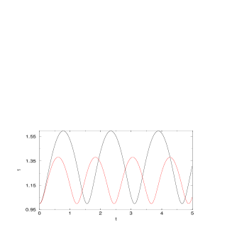
FIG. 1.: Perspective view of $\tau$ showing the initially nonsingular and oscillating behavior of the solutions

case 3. $\Lambda<0$ and $\lambda<0$. The solution is singular at initial moment, that is

$$\lim\limits_{t\to 0}\tau\approx[\sqrt{-3\lambda n^{2}C_{0}^{n}/4}t]^{2/n}$$ (51)

and at $t\to\infty$ asymptotic isotropization takes place since

$$\lim\limits_{t\to\infty}\tau\approx e^{\sqrt{3\Lambda}t}.$$ (52)

case 4. $\Lambda>0$ and $\lambda<0$. Solution is initially singular and coincides with (51) and bound from the above, i.e., oscillating, since

$$\lim\limits_{t\to\infty}\tau\approx{\rm sin}\sqrt{3\Lambda}t.$$ (53)

4 Conclusion

Within the framework of the simplest nonlinear model of spinor field it has been shown that the $\Lambda$ term plays very important role in Bianchi-I cosmology. In particular, it invokes oscillations in the model which is not the case when $\Lambda$ term remain absent. Growing interest in studying the role $\Lambda$ term by present day physicists of various discipline witnesses its fundamental value. For details on time depending $\Lambda$ term one may consult [25] and references therein.

REFERENCES

• [1] L. Parker, Phys. Rev. 183, 1057 (1969).
• [2] L. Parker, Phys. Rev. D 3, 346 (1971).
• [3] C.W. Misner, Astrophys. J. 151, 431 (1968).
• [4] B.L. Hu and L. Parker, Phys. Rev. D 17, 933 (1978).
• [5] V.A. Belinskii,  E.M. Lifshitz and I.M. Khalatnikov, Adv. Phys. 19, 525 (1970).
• [6] K.C. Jacobs, Astrophys. J. 153, 661 (1968).
• [7] L.P. Chimento and M.S. Mollerach, Phys. Lett. A 121, 7 (1987).
• [8] M.A. Castagnino,  C.D. El Hasi,  F.D. Mazzitelli and J.P. Paz, Phys. Lett. A 128, 25 (1988).
• [9] B.L. Hu, Phys. Rev. D 18, 968 (1978).
• [10] P.G. Miedema and W.A. van Leeuwen, Phys. Rev. D 47, 3151 (1993).
• [11] H.T. Cho, Phys. Rev. D 52, 5445 (1995).
• [12] G.N. Shikin, Preprint IPBRAE, Acad. Sci. USSR 19, 21 p. (1991).
• [13] Yu.P. Rybakov,  B. Saha and G.N. Shikin, PFU Reports, Phys., 2, (2), 61 (1994).
• [14] Yu.P. Rybakov,  B. Saha and G.N. Shikin, Commun in Theor. Phys. 3, 199 (1994).
• [15] B. Saha and G.N. Shikin, J. Math. Phys. 38, 5305 (1997).
• [16] R. Alvarado,  Yu.P. Rybakov,  B. Saha and G.N. Shikin, JINR Preprint E2-95-16, 11 p. (1995), Commun in Theor. Phys. 4, (2), 247 (1995), gr-qc/9603035.
• [17] R. Alvarado,  Yu.P. Rybakov,  B. Saha and G.N. Shikin, Izvestia VUZob 38,(7) 53 (1995).
• [18] B. Saha, and G.N. Shikin, Gen. Relat. Grav. 29, 1099 (1997).
• [19] A. Einstein, Sitz. Ber. Preuss. Acad. Wiss. (1917) and (1919).
• [20] V.A. Zhelnorovich, Spinor theory and its application in physics and mechanics (Nauka, Moscow, 1982).
• [21] D. Brill, and J. Wheeler, Rev. Mod. Phys. 29, 465 (1957).
• [22] Ya.B. Zeldovich, and I.D. Novikov, Structure and evolution of the Universe (Nauka, Moscow, 1975).
• [23] N.N. Bogoliubov, and D.V. Shirkov, Introduction to the theory of quantized fields (Nauka, Moscow, 1976).
• [24] E. Kamke, Differentialgleichungen losungsmethoden und losungen (Leipzig, 1957).
• [25] Bijan Saha, gr-qc/0009002