Description of Supernova Data in Conformal Cosmology without Cosmological Constant

Abstract

We consider cosmological consequences of a conformal - invariant formulation of Einstein’s General Relativity where instead of the scale factor of the spatial metrics in the action functional a massless scalar (dilaton) field occurs which scales all masses including the Planck mass. Instead of the expansion of the universe we obtain the Hoyle-Narlikar type of mass evolution, where the temperature history of the universe is replaced by the mass history. We show that this conformal - invariant cosmological model gives a satisfactory description of the new supernova Ia data for the effective magnitude - redshift relation without a cosmological constant and make a prediction for the high-redshift behavior which deviates from that of standard cosmology for $z>1.7$.

1. Introduction

The recent data for the luminosity-redshift relation obtained by the supernova cosmology project (SCP) [1] point to an accelerated expansion of the universe within the standard Friedman-Robertson-Walker (FRW) cosmological model. Since the fluctuations of the microwave background radiation [2] provide evidence for a flat universe a finite value of the cosmological constant $\Lambda$ has been introduced [3] which raises to the cosmic coincidence (or fine-tuning) problem  [4]. A most common approach to the solution of this problem is to allow a time dependence of the cosmological constant (“Quintessence” [5, 4]), the speed of light [6] or the fine structure constant [7].

The present paper is devoted to an alternative description of the new cosmological supernova data without a $\Lambda$- term as evidence for Weyl’s geometry of similarity [8], where Einstein’s theory takes the form of the conformal - invariant theory of a massless scalar field [9, 10, 11, 12, 13, 14].

As it has been shown by Weyl [8] already in 1918, conformal - invariant theories correspond to the relative standard of measurement of a conformal - invariant ratio of two intervals, given in the geometry of similarity as a manifold of Riemannian geometries connected by conformal transformations. This ratio depends on nine components of the metrics whereas the tenth component became the scalar dilaton field that can not be removed by the choice of the gauge. In the current literature [15, 16] (where the dilaton action is the basis of some speculations on the unification of Einstein’s gravity with the standard model of electroweak and strong interactions including modern theories of supergravity) this peculiarity of the conformal - invariant version of Einstein’s dynamics has been overlooked.

The energy constraint converts this dilaton into a time-like classical evolution parameter which scales all masses including the Planck mass. In the conformal cosmology (CC), the evolution of the value of the massless dilaton field (in the homogeneous approximation) corresponds to that of the scale factor in standard cosmology (SC). Thus, the CC is a field version of the Hoyle-Narlikar cosmology [17], where the redshift reflects the change of the atomic energy levels in the evolution process of the elementary particle masses determined by that of the scalar dilaton field [12, 17, 18]. The CC describes the evolution in the conformal time, which has a dynamics different from that of the standard Friedmann model.

In the present paper we will discuss as an observational argument in favour of the CC scenario that the Hubble diagram (effective magnitude - redshift- relation: $m(z)$) including the recent SCP data [1] can be described without a cosmological constant.

2. Conformal General Relativity

The principle of relativity of all standards of measurement can be incorporated into the unified theory through the Weyl geometry of similarity as a manifold of conformal - equivalent Riemannian geometries. To escape defects of the first Weyl version of 1918 [8], we use the scalar-tensor conformal invariant $(\hat{g}_{\mu\nu}=w^{2}g_{\mu\nu})$ where $w$ is a dilaton scalar field described by the Penrose-Chernikov-Tagirov (PCT) action [9]

$$S_{CGR} = -\int\limits d^{4}x\sqrt{-\hat{g}}\frac{1}{6}R(\hat{g})$$ (1)

$$= \int d^{4}x\left[-\sqrt{-g}\frac{w^{2}}{6}R(g)+w\partial_{\mu}(\sqrt{-g}g^{\mu\nu}\partial_{\nu}w)\right]~{}$$

with negative sign. The action and conformal - invariant equations of this theory coincide with the ones of Einstein’s general relativity (GR) expressed in terms of the conformal - invariant Lichnerowicz variables $F_{(n)}$, including the metric $g$ [19]

$$F^{L}_{(n)}=||{}^{(3)}g||^{-n/6}F_{(n)}~{},~{}~{}~{}~{}~{}(ds^{L})^{2}=g^{L}_{\mu\nu}dx^{\mu}dx^{\nu},~{}~{}~{}~{}||{}^{(3)}g^{L}||=1~{},$$ (2)

where ${}^{(3)}g_{ij}$ are the 3-dimensional metric components, $(n)$ is the conformal weight for a tensor $(n=2)$, vector $(n=0)$, spinor $(n=-3/2)$, and scalar $(n=-1)$ field. The role of the dilaton field in GR is played by the scale-metric field

$$w_{g}=||{}^{(3)}g||^{1/6}M_{\rm Planck}\sqrt{\frac{3}{8\pi}}~{}.$$ (3)

Therefore, we call this theory the conformal general relativity (CGR).

In contrast to Einstein’s general relativity theory, in Weyl’s conformal relativity we can measure only a ratio of two Einstein intervals that depends only on nine components of the metric tensor. This means that the conformal invariance allows us to remove only one component of the metric tensor using the scale-free Lichnerowicz conformal - invariant field variables (2). We show that the conformal invariance of the action, the variables, and the measurable quantities gives us an opportunity to solve the problems of modern cosmology without inflation by the definition of the observables as conformal - invariant quantities. We introduce the conformal time, the conformal (coordinate) distance, the conformal density, the conformal pressure, etc. using instead of the FRW cosmic scale factor the homogeneous dilaton field which scales all masses in the universe.

After the introduction of the CGR for an empty universe we give now to the action of the matter fields in a conformal invariant formulation of the Standard Model (SM)

$$S_{CSM} = \int d^{4}x\sqrt{-g}\left[\frac{|\Phi|^{2}}{6}R(g)+{\cal L}^{SM}_{0}(g,\{v_{i}\},\{\psi_{j}\},\Phi)+{\cal L}_{\rm Higgs}(|\Phi|,w)\right]~{},$$ (4)

where ${\cal L}^{SM}_{\lambda}(g,\{v_{i}\},\{\psi_{j}\},\Phi)$ is the SM Lagrangian with the metric tensor $g$, the Higgs field $\Phi$, the vector boson fields $\{v_{i}\}$, the spinor fields $\{\psi_{j}\}$ and the coupling constant $\lambda$ of the conventional Higgs potential. The latter one has to be replaced by the conformal - invariant one

$${\cal L}_{\rm Higgs}(\Phi,w)=-\lambda\left[\left(|\Phi|\right)^{2}-C^{2}(w)\right]^{2}~{},$$ (5)

where the mass term of the Higgs field $C(w)=y_{\rm Higgs}w$ is rescaled by the cosmological dilaton $w$. The conformal - invariant interactions of the dilaton and the Higgs doublet form the effective Newton coupling in the gravitational Lagrangian

$$\frac{|\Phi|^{2}-w^{2}}{6}R~{}.$$ (6)

From this term the necessity becomes obvious to introduce the modulus $\phi$ and the mixing angle $\chi$ of the the dilaton-Higgs mixing [20] as new variables by

$$w=\phi~{}\cosh\chi,~{}~{}~{}~{}~{}~{}|\Phi|=\phi~{}\sinh\chi~{}~{},$$ (7)

so that the total Lagrangian of our conformal cosmology model takes the form

$${\cal L} = {\cal L}_{CGR}+{\cal L}_{CSM}$$ (8)

$$= -\frac{\phi^{2}}{6}R-\partial_{\mu}\phi\partial^{\mu}\phi+\phi^{2}\partial_{\mu}\chi\partial^{\mu}\chi+{\cal L}_{\rm Higgs}(\phi,\chi)+\bar{\psi}_{e}y_{e}\phi\sinh\chi\psi_{e}+...~{},$$

where the Higgs Lagrangian

$${\cal L}_{\rm Higgs}(\phi,\chi)=-\lambda\phi^{4}\left[\sinh^{2}\chi-y^{2}_{\rm Higgs}\cosh^{2}\chi\right]^{2}$$ (9)

describes the conformal - invariant Higgs effect of the spontaneous SU(2) symmetry breaking

$$\frac{\partial{\cal L}_{\rm Higgs}}{\partial\chi}=0~{}\Rightarrow\chi_{1}=0,~{}~{}~{}~{}\sinh\chi_{2,3}=\pm\frac{y_{\rm Higgs}}{\sqrt{1-y^{2}_{\rm Higgs}}}\sim 10^{-17}~{}$$ (10)

corresponding to the latter pair of solutions ($\chi_{2,3}$). The masses of elementary particles are also scaled by the modulus of the dilaton-Higgs mixing. There are two ways to obtain the Standard Model. The simplest way is to use a scale transformation to convert this modulus into a constant (instead of the Lichnerowicz gauge (2))

$$\phi(x_{0},x)=\varphi_{0}=M_{\rm Planck}\sqrt{\frac{3}{8\pi}}~{}.$$ (11)

In this case the Lagrangian (8) goes over into the Einstein-Hilbert one with

$$y_{\rm Higgs}=\frac{m_{X}}{\varphi_{0}}\sim 10^{-17}~{}.$$ (12)

In the limit of infinite Planck mass the SM sector decouples from the gravitational one and takes the standard renormalizable form with the Higgs potential

$$-\lambda(X^{2}-{m}^{2}_{X})^{2}+O\left(\frac{1}{M_{\rm Planck}}\right)~{},$$ (13)

where the notations $\varphi_{0}\chi=X$ and $\varphi_{0}y_{\rm Higgs}={m}_{X}$ have been introduced for the Higgs field and its mass term, respectively. However, the gauge (11) violates the conformal symmetry of the equations of motion and introduces an absolute standard of measurement of geometric intervals depending on ten components. This way leads to the standard cosmology.

The second way is to choose the Weyl relative standard of measurement of intervals depending on nine components of the metric tensor in the general case. This way is compatible with the Lichnerowicz gauge (2) that does not violate the conformal symmetry of the equations of motion in the conformal - invariant theory considered. In this case, the equality (11) follows from the energy constraint and means the current (non-fundamental) status of Planck mass [14]. The Weyl relative standard of measurement leads to the conformal cosmology [12].

3. Cosmological solutions for the dilaton - Higgs dynamics

It is well-known that the homogeneous and isotropic approximation to GR is described by the metric

$$ds^{2}=g_{00}(x_{0})dx^{0}dx^{0}-a^{2}(x^{0})dx^{i}dx^{i}=a^{2}(x^{0})(ds^{L})^{2}~{},$$ (14)

where $dt=\sqrt{g_{00}}dx_{0}$ is the Friedmann time interval.

In this approximation CGR is described by the flat conformal space-time

$$(ds^{L})^{2}=d\eta^{2}-dx_{i}^{2}~{},$$ (15)

where $d\eta=\sqrt{g^{L}_{00}}dx_{0}$ is the conformal time interval and the abbreviation $N_{0}=\sqrt{g^{L}_{00}}$ will be used. For simplicity we will restrict us here to the discussion of flat space.

The rôle of the cosmic scale factor in CGR is played by the zero momentum mode of the Fourier decomposition of the dilaton field,

$$\varphi(x_{0})=\frac{1}{V}\int d^{3}x\phi^{L}(x_{0},\vec{x})~{},$$ (16)

that scales (as we have seen before) all masses of elementary particles including the Planck mass. The infrared interaction of the complete set of local independent variables $\{f\}$ with this dilaton zero mode $\varphi(x_{0})$ is taken into account exactly, and it is the subject of the well-known problem of the cosmological creation of particles in terms of the conformal variables (2), see also [22]. From the CGR action, we obtain the equation of motion for the dilaton field as the conformal analogue of the Friedmann equation for the evolution of the universe

$$\frac{\partial S}{\partial N_{0}}=0~{}~{}~{}~{}~{}\Rightarrow~{}~{}~{}~{}~{}(\varphi^{\prime})^{2}=\rho(\varphi)~{},$$ (17)

where the prime denotes the derivative with respect to the conformal time $\eta$.

$$\rho(\varphi)=\frac{1}{V}\int d^{3}xT_{00}(\varphi)$$ (18)

is the conformal energy density which is connected with the SC one by $\rho(\varphi)=a^{4}~{}\rho_{SC}~{}$, where $a=\varphi/\varphi_{0}$.

The cosmic evolution of dilaton masses leads to the redshift of energy levels of star atoms [17] as a function of the elapsed conformal time. We can introduce the Hubble parameter of the CC model, $H_{0}=\varphi^{\prime}(\eta_{0})/\varphi(\eta_{0})$, which can be used to fix the integration constant occuring in the solution of the evolution equation (17) with the present day value of the dilaton $\varphi_{0}=\varphi(\eta_{0})$

$$\varphi_{0}=\frac{\sqrt{\rho(\varphi_{0})}}{H_{0}}=M_{\rm Planck}\sqrt{\frac{3}{8\pi}}~{}.$$ (19)

In CC, the Planck mass is subject to cosmic evolution and thus not a fundamental parameter that could be used to describe the beginning of the Universe.

The field theory reproduces all regimes of the classical SC in their conformal versions. In particular, the theory of the free field describes all the equations of state that are known in the standard cosmology: the rigid state ($p_{\rm Rigid}=\rho_{\rm Rigid}(\varphi)={\rm const}/\varphi^{2}$), the radiation state ($p_{\rm Radiation}=\rho_{\rm Radiation}/3={\rm const}$), and the matter state ($p_{\rm Matter}=0,~{}~{}\rho_{\rm Matter}={\rm const}\varphi$) [13, 14]. The origin of the rigid state are excitations of the homogeneous graviton and the dilaton - Higgs field mixing; the radiation state corresponds to excitations of other massless fields and the matter one to those of massive fields.

Now we can ask: What is the best regime for a description of the latest Supernova data on the luminosity distance - redshift relation and is this regime compatible with the other cosmological data, like the CMB radiation and element abundances?

4. Luminosity distance - redshift relation

Let us establish the correspondence between the SC and the CC determined by the evolution of the dilaton (17), where the time $\eta$, the density $\rho(\varphi)$, and the Hubble parameter $H_{0}$ are treated as measurable quantities. Let us introduce the standard cosmological definition of the redshift and density parameter

$$1+z\equiv\frac{1}{a(\eta)}=\frac{\varphi_{0}}{\varphi(\eta)}~{},~{}~{}~{}\Omega(z)=\frac{\rho(\varphi)}{\rho(\varphi_{0})},$$ (20)

where $\Omega(0)=1$ is assumed. The density parameter $\Omega(z)$ is determined in both the SC and the CC as

$$\Omega(z)=\Omega_{\rm Rigid}(1+z)^{2}+\Omega_{\rm Radiation}+\frac{\Omega_{\rm Matter}}{(1+z)}+\frac{\Omega_{\Lambda}}{(1+z)^{4}}~{}.$$ (21)

We added here the $\Omega_{\Lambda}$-term that corresponds to the $\lambda\varphi^{4}$ interaction in the conformal action in order to have the complete analogy with the standard cosmology. Then the equation (17) takes the form

$$H_{0}\frac{d\eta}{dz}=\frac{1}{(1+z)^{2}}\frac{1}{\sqrt{\Omega(z)}}~{},$$ (22)

and determines the dependence of the conformal time on the redshift factor. This equation is valid also for the conformal time - redshift relation in the SC where this conformal time is used for description of a light ray.

A light ray traces a null geodesic, i.e. a path for which the conformal interval $(ds^{L})^{2}=0$ thus satisfying the equation ${dr}/{d\eta}=1$. As a result we obtain for the coordinate distance as a function of the redshift

$$H_{0}r(z)=\int_{0}^{z}\frac{dz^{\prime}}{(1+z^{\prime})^{2}}\frac{1}{\sqrt{\Omega(z^{\prime})}}.$$ (23)

The equation (23) coincides with the similar relation between coordinate distance and redshift in SC.

In the comparison with the stationary space in SC and stationary masses in CC, a part of photons is lost. To restore the full luminosity in both SC and CC we should multiply the coordinate distance by the factor $(1+z)^{2}$. This factor comes from the evolution of the angular size of the light cone of emitted photons in SC, and from the increase of the angular size of the light cone of absorbed photons in CC.

However, in SC we have an additional factor $(1+z)^{-1}$ due to the expansion of the universe, as measurable distances in SC are related to measurable distances in CC (that coincide with the coordinate ones) by the relation

$$\ell={a}\int\limits\frac{dt}{a}=\frac{r}{1+z}~{}.$$ (24)

Thus we obtain the relations

$$\ell_{\rm SC}(z)=(1+z)^{2}\ell=(1+z)r(z)~{},$$ (25)

$$\ell_{\rm CC}(z)=(1+z)^{2}r(z)~{}.$$ (26)

This means that the observational data are described by different regimes in SC and CC. For example, the rigid state (i.e. $\Omega_{\rm Rigid}=1$) gives the relation

$$\ell_{\rm CC}(z)=z+\frac{z^{2}}{2}~{}.$$ (27)

In Fig. 1 we compare the results of the SC and CC for the effective magnitude-redshift relation: $m(z)=5\log{[H_{0}\ell(z)]}+{\cal M}$ , where ${\cal M}$ is a constant, with recent experimental data for distant supernovae [1, 21]. Within the CC model the pure rigid state of dilaton-Higgs dynamics without cosmological constant gives the best description and is equivalent to the SC fit up to the SN1997ff point.

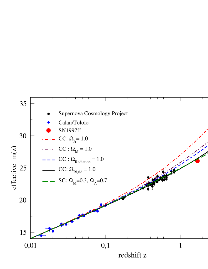
Figure 1: $m(z)$-relation for a flat universe model in SC and CC. The data points include those from 42 high-redshift Type Ia supernovae [1] and that of the recently reported farthest supernova SN1997ff [21]. An optimal fit to these data within the SC requires a cosmological constant $\Omega_{\Lambda}=0.7$, whereas in the CC these data require the dominance of the rigid state.

5. Cold Universe Scenario

In this section we want to discuss the consistency of the here described CC scenario of a nonexpanding Universe, in which the observed redshift of spectra is due to time-dependent elementary particle masses, with other cosmological observations such as the CMB radiation and the distribution of elements.

In the limit of the Early Universe, $\varphi\Rightarrow 0$, the CGR action also gives the most singular rigid state ${\rho}/{\rho_{0}}=\Omega_{\rm Rigid}(z+1)^{2}$ and the primordial motion of the dilaton described before

$$\varphi^{2}(\eta) = \varphi^{2}_{I}[1+2H_{I}\eta]=\frac{\varphi^{2}_{0}}{(1+z)^{2}}~{},$$

$$H(z) = \frac{\varphi^{\prime}}{\varphi}=H_{0}(1+z)^{2}~{}.$$ (28)

At the point of coincidence of the Hubble parameter of this motion with the mass of vector bosons $m_{v}(z)\sim H(z)$, there occurs the intensive creation of longitudinal vector bosons, see [23]. Fast thermal equilibration of this boson system takes place since for the inverse relaxation time holds $\eta^{-1}_{\rm relaxation}=\sigma_{\rm scat.}n_{v}\geq H(z)$, and therefore the density of created vector bosons $n_{v}$ defines an equilibrium temperature which appears to be an the integral of motion of the cosmic evolution $T_{\rm eq}\!\simeq\![m^{2}_{v}(z)H(z)]^{1/3}\!\simeq\!(m_{W}^{2}H_{0})^{1/3}=2.7K\!\sim\!H_{I}$. This is a surprisingly good agreement of $T_{\rm eq}$ with the CMB radiation temperature.

It is worth to emphasize this difference between the CC model and the SC ones: In conformal cosmology, the CMB temperature remains constant (cold scenario) but the masses evolve throughout the history of the universe due to the time dependence of the dilaton field

$$m_{\rm era}{(z_{\rm era})}=\frac{m_{\rm era}(0)}{(1+z_{\rm era})}=T_{\rm eq}~{},$$ (29)

where $m_{\rm era}(0)$ is the present-day value of a characteristic energy (mass) scale determining the onset of an era of the universe evolution.

Eq. (29) has the important consequence that all those physical processes which concern the chemical composition of the universe and which depend basically on Boltzmann factors with the argument $(m/T)$ cannot distinguish between the mass history of conformal cosmology and the temperature history of standard cosmology due to the relations

$$\frac{m(z)}{T(0)}=\frac{m(0)}{(1+z)T(0)}=\frac{m(0)}{T(z)}~{}.$$

This formula makes transparent that in this order of approximation a $z$-history of masses with invariant temperatures in the rigid state of CC is equivalent to a $z$-history of temperatures with invariant masses in the radiation stage of SC. We expect therefore that the conformal cosmology will be as successful as the standard cosmology in the radiation stage for describing, e.g., the neutron-proton ratio and the primordial element abundances.

An important new feature of the conformal cosmology relative to the standard one is the absence of the Planck era, since the Planck mass is not a fundamental parameter but only the present-day value of the dilaton field [12].

6. Conclusion

We have presented an approach according to which the new supernova data can be interpreted as evidence for a new type of geometry in Einstein’s theory rather then a new type of matter. This geometry corresponds to the relative standard of measurement and to a conformal cosmology with constant three-volume. In this cosmology, the dilaton field scales all masses and its evolution is responsible for observable phenomena like the redshift of spectra from distant galaxies. The evolution of all masses replaces the familiar evolution of the scale factor in standard cosmologies. The infrared dilaton - elementary particle interaction leads to particle creation [23] and in turn to the occurence of the CMB radiation with a temperature of $2.7$ K not changed ever since.

We have defined the cosmological parameters in the conformal cosmology, and we have found that the effective magnitude - redshift relation (Hubble diagram) for a rigid state which originates from the dilaton - Higgs dynamics describes the recent observational data for distant (high-redshift) supernovae including the farthest one at $z=1.7$. While in the standard FRW cosmology interpretation a $\Lambda$ - term (or a quintessential analogue) is needed, which entails a transition from decelerated to accelerated expansion at about $z\sim 1.7$, the cosmology presented here does not need a $\Lambda$ - term. Both cosmologies make different predictions for the behaviour at $z>1.7$. Provided that the CSM with a Higgs potential gives a correct description of the matter sector, our findings suggest that new data at higher redshift could discriminate between the alternative cosmological interpretations of the luminosity - redshift relation and answer the question: Is the universe expanding or not?

Acknowledgement

We thank Dr. A. Gusev and Prof. S. Vinitsky for fruitful discussions. One of us (V.N.P.) acknowledges support by the Ministery for Education, Science and Culture in Mecklenburg - Western Pommerania and thanks for the hospitality of the University of Rostock where this work has been completed. D.P. thanks the RFBR (grant 00-02-81023 Bel$\_a$) for support.

References

-
[1]
A. G. Riess et al., Astron. J. 116 (1998) 1009;
S. Perlmutter et al., Astrophys. J. 517 (1999) 565. - [2] J. R. Bond et al. (MaxiBoom collaboration), CMB Analysis of Boomerang & Maxima & the Cosmic Parameters , in: Proc. IAU Symposium 201 (PASP), CITA-2000-65 (2000). [astro-ph/0011378].
- [3] S. Perlmutter, M. S. Turner and M. White, Phys. Rev. Lett. 83 (1999) 670.
- [4] I. Zlatev, L. Wang and P. J. Steinhardt, Phys. Rev. Lett. 82 (1999) 896.
- [5] C. Wetterich, Nucl. Phys. B 302 (1988) 668.
- [6] J. D. Barrow, H. B. Sandvik, J. Magueijo, The Behaviour of Varying-Alpha Cosmologies, astro-ph/0109414.
- [7] J. W. Moffat, A Model of Varying Fine Structure Constant and Varying Speed of Light, astro-ph/0109350, and Refs. therein.
- [8] H. Weyl, Sitzungsber. d. Berl. Akad. (1918) 465.
-
[9]
R. Penrose, Relativity, Groups and Topology,
(Gordon and Breach, London 1964);
N. Chernikov and E. Tagirov, Ann. Inst. Henri Poincarè 9 (1968) 109. - [10] J. D. Bekenstein, Ann. Phys. (NY) 82 (1974) 535.
- [11] V. Pervushin et al., Phys. Lett. B 365 (1996) 35.
- [12] M. Pawlowski, V. V. Papoyan, V. N. Pervushin and V. I. Smirichinski, Phys. Lett. B 444 (1998) 293.
- [13] V. N. Pervushin and V. I. Smirichinski, J. Phys. A: Math. Gen. 32 (1999) 6191.
-
[14]
M. Pawlowski, V. N. Pervushin, Int. J. Mod. Phys. 16 (2001) 1715,
[hep-th/0006116];
V. N. Pervushin and D. V. Proskurin, Gravitation and Cosmology, 7 (2001) 89. - [15] M. Pawlowski and R. Raczka, Found. of Phys. 24 (1994) 1305.
- [16] R. Kallosh, L. Kofman, A. Linde and A. Van Proeyen, Class. Quant. Grav. 17 (2000) 4269.
- [17] J. V. Narlikar, Space Sci. Rev. 50 (1989) 523.
- [18] D. Behnke, D. Blaschke, V. Pervushin, D. Proskurin and A. Zakharov, Cosmological Consequences of Conformal General Relativity, [gr-qc/0011091].
- [19] A. Lichnerowicz, Journ. Math. Pures and Appl. B 37 (1944) 23.
- [20] V. N. Pervushin et al., Phys. Lett. B 365 (1996) 35.
- [21] A. G. Riess et al., The Farthest Known Supernova: Support for an Accelerating Universe and a Glimpse of the Epoch of Deceleration, Astrophys. J. (2001) in press, [astro-ph/0104455].
-
[22]
G. L. Parker, Phys. Rev. Lett. 21 (1968) 562,
Phys. Rev. 183 (1969) 1057,
Phys. Rev. D 3 (1971) 346;
Ya. B. Zel’dovich, A. A. Starobinski, ZHETF 61 (1971) 2161;
A. A. Grib, S. G. Mamaev, V. M. Mostepanenko, Quantum effects in intensive external fields, (Moscow, Atomizdat, 1980) (in Russian). - [23] D. Blaschke, V. Pervushin, D. Proskurin, S. Vinitsky and A. Gusev, Cosmological Creation of Vector Bosons and Fermions, Dubna Preprint JINR-E2-2001-52; [gr-qc/0103114].