Abstract

The Einstein equations for a perfect fluid spatially homogeneous spacetime are studied in a unified manner by retaining the generality of certain parameters whose discrete values correspond to the various Bianchi types of spatial homogeneity. A parameter dependent decomposition of the metric variables adapted to the symmetry breaking effects of the nonabelian Bianchi types on the “free dynamics” leads to a reduction of the equations of motion for those variables to a 2-dimensional time dependent Hamiltonian system containing various time dependent potentials which are explicitly described and diagrammed. These potentials are extremely useful in deducing the gross features of the evolution of the metric variables.

1 Introduction

Although interest in spatially homogeneous cosmological models peaked in the early seventies, it was not until the late seventies that a more unified picture of the dynamics of these models developed, following the proper recognition of the role played in the problem by the gauge freedom of general relativity [1–3]. Since a number of books [4,5] and review articles [6–9] exist which discuss spatially homogeneous cosmology at various levels and from various points of view, it seems appropriate here to emphasize certain aspects of the subject which are not well covered in the literature. Remarkably there is still something new left to say on this topic nearly a decade after its most active period of research. The present discussion will seek to generalize many concepts which have already appeared in the context of particular symmetry types or special initial data and fit them together into a single unified picture of spatially homogeneous dynamics. It should be emphasized that although spatially homogeneous cosmological models are usually studied for a (nearly) discrete set of parameter values corresponding to the (nearly) discrete set of Bianchi types [10–14], both the metric and field equations depend analytically on a 4-dimensional space of essential parameters (of which at most three may be simultaneously nonzero). By varying these parameters continuously, one may deform each of the various symmetry types into each other and thus relate properties of one Bianchi type to those of another, the more specialized symmetry types occurring as singular limits of more general types.

Lagrangian or Hamiltonian techniques enable one to associate a finite dimensional classical mechanical system with the ordinary differential equations equivalent to the spatially homogeneous Einstein equations and thus offer a convenient means of visualizing the dynamics and of understanding its qualitative features. These techniques, which provide the framework of this exposition, were pioneered by Misner [15–18] and followed through by Ryan [19–23], leading to an alternative but equivalent description [24] of the qualitative results obtained by Lifshitz, Khalatnikov and Belinsky [25–29] for the evolution of certain spatially homogeneous cosmological models near the initial singularity using piecewise analytic approximations. This latter work was later confirmed and extended by Bogoyavlensky, Novikov and Peresetsky using powerful techniques from the qualitative theory of differential equations [30–35]. Qualitative studies of various perfect fluid models including the regime away from the initial singularity should also be noted [36–40].

The present discussion has as its foundation previous papers of the author [1–3, 41–43]. No attempt will be made to review the large body of important work which preceded them. References [4–9] adequately serve this function. In particular the bibliographies of the Ryan-Shepley book [5] and the recent review by MacCallum [9] provide an exhaustive list of relevant research papers.

It turns out that the key to our problem is a simple adage of mathematical physics: whenever a symmetric matrix is encountered, diagonalize it. First one diagonalizes the symmetric tensor density associated with the structure constant tensor whose components completely determine locally the type of spatial homogeneity. The three diagonal components plus an additional parameter characterizing the trace of the structure constant tensor are the four parameters referred to above. Next one diagonalizes the component matrix of the spatial metric, maintaining the values of these parameters. This leads to a decomposition of the gravitational configuration space variables (namely the component matrix of the spatial metric) into two sets of three variables, one set parametrizing the diagonal values of the metric component matrix which are readily interpreted in terms of the action of the 3-dimensional scale group (independent rescaling of the unit of length along orthogonal directions) and another set specifying the diagonalizing matrix. This decomposition incredibly simplifies the field equations since the diagonalizing variables correspond to pure gauge directions, reflecting the effect on the metric variables of spatial diffeomorphisms which are compatible with the spatial homogeneity. Scalar functions such as the spatial scalar curvature which are gauge invariant depend at most on some of the diagonal variables, for example. Finally one diagonalizes the DeWitt metric [44] on the configuration space ${\cal M}$ of spatial metric component matrices by choosing an orthogonal basis of the Lie algebras of the scale group and of the 3-dimensional group $\hat{G}$ used in the metric diagonalization; the DeWitt metric is important since the “free dynamics” is equivalent to geodesic motion for this metric. The advantages of diagonal matrices over general symmetric matrices are obvious; all matrix operations (multiplication, determinant, inverse) become trivial and functions of these matrices have a much simpler dependence on the individual components. Diagonalizing a quadratic form kinetic energy function also greatly simplifies the equations of motion.

A familiar example from classical mechanics which proves useful as an analogy is the problem of the motion of a rigid body [45,46]. Such an analogy was in fact first introduced for general spacetimes by Fischer and Marsden [47] in their original discussion of the role of the lapse and shift in the three-plus-one formulation of the Einstein equations. It is even more appropriate for the spatially homogeneous spacetimes where the correspondence is nearly complete. The usual synchronous gauge spatial frame is analogous to the space-fixed axes in the rigid body problem. The “diagonal gauge” spatial frame which diagonalizes both the spatial metric and the symmetric tensor density associated with the structure constant tensor corresponds to the body-fixed axes which diagonalize the moment of inertia tensor. The special orthogonal group $SO(3,R)$ generalizes to the relevant 3-dimensional diagonalizing matrix group $\hat{G}$. Since the components of the structure constant tensor must remain fixed under its action, this group is a matrix representation of a subgroup of the special automorphism group of the given Bianchi type Lie algebra (the subgroup is unimodular since its Lie algebra is required to be offdiagonal). The concept of angular velocity also has an analogue which is closely related to the shift vector field whose associated time dependent spatial diffeomorphism drags the synchronous spatial frame into the diagonal gauge spatial frame by inducing the time dependent frame transformation which orthogonalizes the spatial frame. However, since the action of $\hat{G}$ on the metric configuration space represents an orbital motion, the situation is more involved.

At this point it is helpful to keep in mind the problem of the nonrelativistic motion of a particle in a spherically symmetric potential (the central force problem). Here the symmetry group $SO(3,R)$ is a subgroup of the group of motions of the Euclidean metric on the configuration space $R^{3}$. By introducing spherical coordinates one separates the configuration space variables into angular variables describing the orbits of $SO(3,R)$, namely 2-spheres except for the fixed point at the origin where the orbit dimension degenerates, and radial variables which describe the directions orthogonal to the orbits. The components of orbital angular momentum arise from evaluating the moment function [40] for the action of $SO(3,R)$ on $R^{3}$ in the standard basis of its Lie algebra and may be interpreted as the inner products of the standard basis of rotational Killing vector fields with the velocity of the system. Since $SO(3,R)$ is a symmetry group of the dynamics, angular momentum is conserved and the problem is then reduced to 1-dimensional radial motion in a new potential, the angular momentum contributing an effective potential (the centrifugal potential) to the original radial potential. When the latter potential is absent, the case of the motion of a free particle, it is of course simplest to consider only radial orbits which lead to the simplest representation of the free (straight line) motion, namely geodesics of the Euclidean metric. This restriction to radial orbits is possible because of the additional translational symmetry which allows one to transform the angular momentum to zero.

In spatially homogeneous dynamics the Euclidean metric on $R^{3}$ is replaced by the Lorentzian DeWitt metric on the 6-dimensional space ${\cal M}$ of spatial metric component matrices. The decomposition of the Euclidean space variables goes over roughly into the 3-dimensional space of “diagonal” variables and the 3-dimensional space of “offdiagonal” variables as described above. The offdiagonal variables describe the orbits of the action on ${\cal M}$ of the matrix group $\hat{G}$ and the diagonal variables describe the orthogonal directions. The moment function for the action of $\hat{G}$ on ${\cal M}$ is the analogue of the orbital angular momentum. Its components in a certain basis of the matrix Lie algebra $\hat{g}$ of $\hat{G}$ will be seen below to correspond to the space-fixed components of the spin angular momentum in the rigid body analogy, thus neatly intertwining these two classical analogies. The free motion (geodesics of the DeWitt metric) is most easily represented as purely diagonal, using the larger isometry group $SL(3,R)$ of the DeWitt metric to transform away the angular momentum associated with any particular subgroup $\hat{G}$. The overall scale of the metric matrix represented by its determinant (product of its diagonal values) corresponds to the single timelike direction and the free motion is subject to an additional energy constraint requiring the geodesic to be null. Apart from the freedom to rescale and translate the affine parameter of these diagonal null geodesics, there is a 1-parameter family of them, parametrized by the angle of revolution of the 2-dimensional null cone in the space of diagonal metric matrices; these are the well known Kasner solutions [48]. However, a geodesic which has zero angular momentum for a particular choice of the group $\hat{G}$ will have nonzero angular momentum for almost all other choices of this group.

In the central force problem the separation of radial and angular variables is clean. In our problem the symmetry group of the free dynamics is $SL(3,R)$ and only the corresponding division of variables into a conformal metric (unit determinant) and a scale variable (the metric determinant which parametrizes the orbits of $SL(3,R)$) is clean. The division of variables into two orthogonal sets of three diagonal variables and three offdiagonal variables is instead highly ambiguous. There is essentially a 2-parameter family of subgroups $\hat{G}$ of $SL(3,R)$ with 3-dimensional offdiagonal matrix Lie algebras whose orbits are almost everywhere transversal to the diagonal submanifold of ${\cal M}$. The orbits of any of these subgroups may be used to perform the decomposition, which is automatically orthogonal with respect to the DeWitt metric. The addition to the free system of the spatial scalar curvature as a potential breaks down the $SL(3,R)$ symmetry uniquely to one of these subgroups in the general case, although some degeneracy remains in some of the more specialized symmetry types (Bianchi types II and V; Bianchi type I is the free system and the symmetry remains unbroken). This breakdown of $SL(3,R)$ symmetry to a particular subgroup $\hat{G}$ depends continuously on the parameters which specify the Lie algebra of the spatial homogeneity group, just as the symmetry breaking scalar curvature potential itself depends continuously on these parameters. When the subgroup $\hat{G}$ has a compact subgroup, the diagonal/offdiagonal decomposition develops a singularity where the orbit dimension degenerates from its generic value three, similar to the coordinate singularity of spherical coordinates at the origin of $R^{3}$. These points of the configuration space turn out to be associated with additional continuous symmetry of the spatial metric; they are protected by angular momentum barriers in the same way as is the origin of $R^{3}$ in the central force problem.

The concept of angular momentum links the rigid body and central force analogies. The time dependent diagonalizing matrix is a curve in the matrix group $\hat{G}$, representing the orbital motion of the system. (In fact the matrix group $\hat{G}$ directly parametrizes the points of each orbit.) The tangent vector of this curve, namely the velocity associated with the offdiagonal variables, represents the orbital velocity of the configuration space point. Given a basis of the matrix Lie algebra $\hat{g}$ of $\hat{G}$, one determines a corresponding basis of the tangent space at the identity and two global frames on $\hat{G}$, one left invariant and one right invariant, which reduce to this basis at the identity. The left and right invariant frame (contravariant) components of the velocity tangent vector correspond respectively to the space-fixed and body-fixed components of the angular velocity in the rigid body analogy. These components are related to each other not by $\hat{G}$ itself as in the previously defined space-fixed and body-fixed components but by the adjoint representation of $\hat{G}$. The association of left and right with space and body assumes that the diagonal gauge frame is related to the synchronous gauge frame by a passive transformation, corresponding to a right action of $\hat{G}$ on ${\cal M}$ and since $\hat{G}$ is identified with its orbits this becomes right translation of $\hat{G}$ into itself.

By the local identification of $\hat{G}$ with its orbits in ${\cal M}$ (the “offdiagonal variables”), one may use the DeWitt metric on the orbit to lower the indices of the velocity tangent vector, leading to what are analogous to the space-fixed (left invariant frame) components and body-fixed (right invariant frame) components of the angular momentum. Thus the frame components of the DeWitt metric along the orbit act as the components of the moment of inertia tensor in the rigid body analogy. The “space-fixed components of the angular momentum” are the inner products of the left invariant frame vectors with the velocity. These vector fields generate the right translations and hence the right action of $\hat{G}$ on ${\cal M}$ and are therefore Killing vector fields of the DeWitt metric. The space-fixed components of the angular momentum are thus the components of the moment function for the action of $\hat{G}$ on ${\cal M}$ and therefore the components of the orbital angular momentum, which are conserved for the free motion. Note, however, that the body-fixed components are related to these constant components by the adjoint transformation and so are in general time dependent. Furthermore, the right invariant frame components of the DeWitt metric must be independent of the orbital variables since right translation is an isometry. By properly choosing the basis of $\hat{g}$, these components may in fact be diagonalized.

One advantage of the present problem over the analogous classical problems is that one is free to reparametrize the time variable by introducing a nontrivial spatially homogeneous lapse function. Lapse functions which depend only on the metric component matrix correspond to conformally rescaling the DeWitt metric and the scalar curvature potential. However, in general the lapse function may also depend on time derivatives of the metric components leading to a much larger freedom in the Hamiltonian system (a freedom not permitted in the Lagrangian approach). Often special choices other than the usual cosmic proper time are suggested by the dynamics which help to simplify its description. Two such choices are the Misner $\Omega$-time [15] related to the logarithm of the metric determinant and his supertime [17], where the lapse is simply related to the metric determinant. The latter choice of time is also crucial to the Belinsky-Lifshitz-Khalatnikov analysis of the dynamics near the initial singularity. For the free dynamics, they are both affine parameters for the geodesic motion.

Of course all of these remarks will become clearer once explicit notation and formulas are introduced. The result of this formal manipulation is a reduction of the Einstein equations to a 2-dimensional Hamiltonian system with time dependent potentials associated with the spatial curvature, with the centrifugal forces arising from the “motion” of the diagonalizing spatial frame, and with the energy-momentum of the source of the gravitational field, here assumed to be a perfect fluid. This system must be supplemented by the equations of motion of the source of course. Explicit diagrams of the various time dependent potentials are extremely useful in deducing the gross features of the evolution of the metric variables; near the initial singularity they may be used to construct “diagrammatic solutions” of the field equations, as done by Ryan for the Bianchi type IX case [20].

The main body of the paper is divided into three sections. In the first of these the parametrized spatially homogeneous spacetime and field equations are introduced. In the second the parametrized decomposition of the metric variables is introduced and used to reduce the Einstein equations to a 2-dimensional time dependent Hamiltonian system. The potentials of this system are then described in detail. In the third section their qualitative effect on the dynamics is discussed.

2 The ${\cal C}_{D}$-parametrized Spatially Homogeneous Spacetime

Before even beginning to discuss spatially homogeneous spacetimes, it is worthwhile introducing some useful facts concerning the smooth action of a Lie group $G$ on a manifold $M$ as a transformation group [49–52]. A left action is just a homomorphism $f:G\to{\cal D}(M)$ from the Lie group into the group of diffeomorphisms of $M$, i.e. for $a\in G$ the corresponding transformation $f_{a}$ satisfies under composition $f_{a_{1}}\circ f_{a_{2}}=f_{a_{1}a_{2}}$. By defining $f^{-1}_{a}\equiv f_{a^{-1}}$ one obtains an antihomomorphism $f^{-1}$ satisfying $f^{-1}_{a_{1}}\circ f^{-1}_{a_{2}}=f^{-1}_{a_{2}a_{1}}$ which is the defining relation for a right action. When $f$ is an isomorphism $(G\simeq f_{G}\equiv\{f_{a}\bigm{|}a\in G\})$ so that only the identity $a_{0}\in G$ acts as the identity transformation on $M$, $f$ is called an effective action. For example, any Lie group acts effectively on itself on the left by left translation $L_{a}(a_{1})=aa_{1}$ and on the right by right translation $R_{a}(a_{1})=a_{1}a$ with $G\simeq L_{G}\simeq R_{G}$. (Note that $R^{-1}:G\to{\cal D}(G)$ is an isomorphism and a left action.) Introducing the redundant but useful notation $a\cdot x\equiv f_{a}(x)$ for the transformation $f_{a}$ acting on $x\in M$, denote the orbit of $x$ by $G\cdot x=\{a\cdot x\bigm{|}a\in G\}$, namely all points which can be reached from $x$ under the action of the group.

Not all of the transformations are effective in moving the point $x$. Let $G_{x}=\{a\in G\bigm{|}a\cdot x=x\}$ be the isotropy subgroup at $x$ of the action of $G$ on $M$, namely the subgroup of $G$ which leaves $x$ fixed. Intuitively one expects that at least locally the orbit of $x$ is in a one-to-one correspondence with the smallest subset of transformations which can move the point $x$ arbitrarily on its orbit. This notion is described by introducing the space $G/G_{x}=\{aG_{x}\bigm{|}a\in G\}$ of left cosets of the subgroup $G_{x}$ in $G$, where each left coset $aG_{x}=\{ab\bigm{|}b\in G_{x}\}$ is an orbit of the right translation action of $G_{x}$ on $G$. All elements of a given coset map $x$ to the same point of $M$ and elements of different cosets necessarily map $x$ to different points as one may easily check. One can therefore extend the domain of the map $f$ from $G$ to $G/G_{x}$ when acting on $x$, i.e. $F_{x}(aG_{x})=f_{a}(x)$ defines a map $F_{x}:G/G_{x}\to G\cdot x$ which turns out to be a diffeomorphism of the left coset space onto the orbit [49]. In particular the dimension of the orbit is the difference in dimension of $G$ and $G_{x}$. Note further that fixing the point in question to be $x_{0}$, so a general point of the orbit may be represented by $x=f_{a}(x_{0})=F_{x_{0}}(aG_{x_{0}})$, then the left action of $G$ on $M$ $\quad x\to f_{a_{1}(x)}=f_{a_{1}a}(x_{0})=F_{x_{0}}(a_{1}aG_{x_{0}})$ corresponds to the left translation $aG_{x_{0}}\to a_{1}aG_{x_{0}}$ on the coset space.

In mathematics any orbit of a transformation group (therefore diffeomorphic to $G/H$ for some subgroup $H$ of $G$) is called a homogeneous space, since all points of the space are equivalent under the transformation group. Here in the context of general relativity, a narrower notion of homogeneous space is required which incorporates not only the equivalence of the points of the space but of the geometry as well. A (pseudo-) Riemannian space $(M,\hbox{\sl g})$ is called homogeneous if it is the orbit of an isometry group (invariance group of the metric g), in which case the action is said to be transitive. A simply transitive action is one in which the isotropy group at every point of the single orbit is trivial (contains only the identity $a_{0}$ of $G$); in this case the orbit and the group are diffeomorphic and the left action of $G$ on $M$ corresponds to left translation on $G$. Using the diffeomorphism $F_{x_{0}}:G\to M$ for an arbitrary point $x_{0}$ of M to pull back the metric from $M$ to $G$, one therefore obtains a left invariant metric on $G$. Thus a homogeneous (pseudo-) Riemannian space with a simply transitive isometry group is equivalent to a left invariant (pseudo-) Riemannian manifold involving that group. (For a right action one simply replaces left by right everywhere in the above discussion; the choice of left or right actions is a matter of convention.)

However, not all transformation groups act transitively and the interesting question about a given action is how the orbits fit together to fill up the entire manifold. One may introduce an integer-valued function $d_{G}(x)\equiv\hbox{dim}(G\cdot x)$ on $M$ whose value gives the dimension of the orbit to which each point belongs; all those orbits of a given dimension form a subspace called a stratum and the partitioning of $M$ into the various strata is called a stratification [53]. Note that it is easy to verify that if $x_{2}=a_{21}\cdot x_{1}$ and $a\in G_{x_{1}}$, then $a^{-1}_{21}aa_{21}\in G_{x_{2}}$, i.e. $G_{x_{2}}=a^{-1}_{21}G_{x_{1}}a_{21}$, so the isotropy subgroups at different points of a given orbit are all conjugate (and therefore isomorphic) subgroups of $G$. Since $d_{G}(x)=\hbox{dim}\ G-\hbox{dim}\ G_{x}$, a decrease in the orbit dimension corresponds to an increase in the isotropy subgroup dimension.

Often the action of a Lie group $G$ on a manifold $M$ describes a symmetry, all points of a given orbit being equivalent in some sense which depends on the context, and one is interested in how things change in the directions “orthogonal” or “oblique” (“transversal”) to the orbits. It is therefore natural to introduce the orbit space $M/G=\{G\cdot x\bigm{|}x\in M\}$; however, due to the varying dimension of the orbits, this is not a manifold. For nice enough actions one can usually choose a subspace of $M$ (a submanifold with or without boundary or a collection of such subspaces which intersects each orbit only once or finitely many times) such that its intersection with the “generic” stratum of maximum dimension orbits is a submanifold whose tangent space is complementary (“transversal”) to the orbit tangent space at each intersection point and hence this submanifold is a local slice for the action on the generic stratum [53]. This “slice” is very helpful in studying objects which are invariant under the group and seem more complicated when studied on the entire space $M$.

For example, consider the rotations about the $z$-axis of $R^{3}$. The group is $SO(2,R)\sim S^{1}$ acting as an isometry subgroup of the Euclidean metric on $R^{3}$, the orbits are circles centered on the $z$-axis and lying in the planes of constant $z$, and the half plane $y=0,x>0$ directly parametrizes the orbit space which is a manifold with boundary. On the other hand the full plane $y=0$ is a manifold intersecting the generic orbits (circles of nonzero radius) twice but having the advantage that the projection of all geodesics of the Euclidean metric onto this manifold are smooth curves, while those which intersect the $z$-axis suffer reflection at the boundary when projected onto the half plane. It is convenient to use the term “slice” to refer to either the plane or the half plane.

The spatially homogeneous spacetimes or “Bianchi cosmologies” which are studied here have a 3-dimensional isometry group $G$ acting simply transitively on a 1-parameter family of spacelike hypersurfaces (the orbits) which provides a natural slicing of the spacetime. Each orbit is a homogeneous Riemannian manifold and therefore isometric to a copy of $G$ equipped with a left invariant Riemannian metric, namely the pullback of the induced spatial metric on the orbit. Rather than maintaining the distinction between $G$ and each orbit, it is simpler to identify the spacetime manifold $M$ with the product manifold $R\times G$, where $R$ is the real line with natural coordinate $t$ which parametrizes the family of copies $G_{t}=\{(t,x)\bigm{|}x\in G\}$ of $G$ in $R\times G$, on each of which $G$ acts by left translation. However, this still leaves open the question of how these left invariant Riemannian manifolds fit together into a spacetime and how the left translations on each copy of $G$ in $R\times G$ fit together into a global action of $G$ on $M$.

One needs to describe a threading of this natural slicing by a congruence of curves in the spacetime (which is nowhere tangent to an orbit) which will be identified with the $t$-lines in $R\times G$, the $t$-coordinate on $R\times G$ corresponding to a given time function for the slicing. Each such identification leads to a different global reference system based on the same natural slicing of the spacetime. In order for the induced metric on each copy of $G$ to be a left invariant metric, the class of threading congruences must be compatible with the action of $G$ on the spacetime. One threading congruence and slicing parametrization is picked out uniquely by the symmetry, namely the invariant congruence of geodesics orthogonal to the orbits, the proper time along these geodesics measured from some initial orbit serving to parametrize the family of orbits. Identifying this parametrized congruence with the $t$-lines of $R\times G$ establishes the so called “synchronous reference system” [48] adapted to the spatial homogeneity, with the action of $G$ on $M=R\times G$ being $t$-independent left translation on each copy of $G$. Any other threading of the slicing may then be viewed as a $t$-dependent diffeomorphism of the family of copies $G_{t}$ of $G$ in $M$ relative to the synchronous threading [47]. Dragging along the $t$-dependent left invariant spatial metric by this diffeomorphism will lead to the $t$-dependent spatial metric in the reference system adapted to the new congruence. This will again be a $t$-dependent left invariant metric only if one restricts the spatial diffeomorphism freedom, i.e. restricts the allowed class of threadings, to be compatible with the group structure of $G$. The compatibility condition is that such diffeomorphisms map the space of left invariant tensor fields on $G$ into themselves. These consist of the left and right translations and the automorphisms of $G$, the latter diffeomorphisms being those which preserve the group multiplication and form a finite dimensional Lie group $Aut(G)=\{h\in{\cal D}(G)\bigm{|}h(a_{1})\,h(a_{2})=h(a_{1}a_{2})\}$ called the automorphism group. The translations and automorphisms together form a semidirect product Lie group [51] $L_{G}\times_{s}Aut(G)=R_{G}\times_{s}Aut(G)\equiv{\cal D}(g)$.

Before discussing in detail the structure of a spatially homogeneous spacetime, it is worth understanding first the homogeneous Riemannian manifolds from which they are constructed. These are left invariant Riemannian 3-manifolds $(G,\hbox{\sl g})$, where g is a left invariant Riemannian metric on the 3-dimensional Lie group $G$. On each Lie group there is a natural identification of the tensor algebra at any given point, say the identity $a_{0}\in G$, with the algebra of either left or right invariant tensor fields. Given a tangent tensor at the identity, one can left (right) translate that tensor all over the group using the differential of the unique left (right) translation which maps the identity to each point of the group, thus obtaining a left (right) invariant tensor field which coincides with the original tensor at the identity. In particular, given a basis $\hat{e}=\{\hat{e}_{a}\}$ of the tangent space at the identity and its dual basis $\{{\hat{\omega}}{}^{a}\}$ of covectors (satisfying $\hat{\omega}^{a}(\hat{e}_{b})=\delta^{a}{}_{b}$), one obtains a global left (right) invariant frame $e=\{e_{a}\}$ ($e=\{\tilde{e}_{a}\}$) and its dual frame $\{\omega^{a}\}$ ($\{{\tilde{\omega}}{}^{a}\}$) of left (right)invariant 1-forms on the group. The components of a given left (right) invariant tensor field in this frame are just the components (namely constants) of the original tensor at the identity with respect to the given basis of the tangent space there. For example, a left invariant Riemannian metric may be expressed in the form

$$\hbox{\sl g}=g_{ab}\ \omega^{a}\otimes\omega^{b},\qquad g_{ab}=\hbox{\sl g}(e_{a},e_{b})$$

where the constant matrix $\hbox{\bf g}=(g_{ab})$ is symmetric and positive-definite. This relation in fact establishes a diffeomorphism (for each left invariant frame $e$) from the space of left invariant metrics on $G$ onto the space ${\cal M}$ of symmetric positive-definite matrices of the given dimension. For dimension three, ${\cal M}$ is a 6-dimensional submanifold of the space $gl(3,R)$ of $3\times 3$ real matrices whose natural basis will be designated by $\{\hbox{\bf e}^{b}{}_{a}\}$, in terms of which a matrix may be represented as $\hbox{\bf A}=(A^{a}{}_{b})=A^{a}{}_{b}\hbox{\bf e}^{b}{}_{a}$.

Let $g$ and $\tilde{g}$ denote the spaces of respectively left and right invariant vector fields on $G$, each isomorphic as a vector space to the tangent space at the identity $TG_{a_{0}}$ and having corresponding bases $e$ and $\tilde{e}$ arising from some basis $\hat{e}$ of $TG_{a_{0}}$. These vector spaces turn out to be closed under the Lie bracket operation and are therefore Lie subalgebras of the infinite dimensional Lie algebra $\hbox{\hbox to0.0pt{\hskip 1.5pt\raise 0.75pt\hbox{--}\hss}${\cal X}$}(G)$ of smooth vector fields on $G$. As a Lie subalgebra of $\hbox{\hbox to0.0pt{\hskip 1.5pt\raise 0.75pt\hbox{--}\hss}${\cal X}$}(G)$, each generates a finite dimensional subgroup of the group ${\cal D}(G)$ of diffeomorphisms of $G$ into itself; $g\ (\tilde{g})$ generates the action of $G$ on itself by right (left) translation, with image diffeomorphism subgroup $R_{G}(L_{G})$. The Lie algebra $g$ of left invariant vector fields on $G$ is referred to as the Lie algebra of the Lie group $G$.

A Lie group $G$ is completely determined locally by the structure of its Lie algebra $g$. Given a basis $e$ of $g$, this structural information is contained in the collection of (constant) components of the structure constant tensor defined by

$$[e_{a},e_{b}]=C^{c}{}_{ab}e_{c}\qquad\hbox{or}\qquad C^{c}{}_{ab}=\omega^{c}([e_{a},e_{b}])\ .$$

Since $e$ is also a global frame on $G$ with dual frame $\{\omega^{a}\}$, a standard formula gives the dual relation

$$d\omega^{a}=-{\textstyle{1\over 2}}C^{a}{}_{bc}\omega^{b}\wedge\,\omega^{c}.$$

Similar formulas hold for $\tilde{e}$ and $\{{\tilde{\omega}}{}^{a}\}$ except for a change in sign of the structure constant tensor components, while $[e_{a},{\tilde{e}}_{b}]=0$ since the diffeomorphism subgroups $R_{G}$ and $L_{G}$ they generate commute with each other due to the associativity of the group multiplication. The structure constant tensor components are not arbitrary but must be antisymmetric in the lower indices and satisfy a quadratic identity imposed by the cyclic Jacobi identity. Let

$${\cal C}=\{C^{a}{}_{bc}\bigm{|}C^{a}_{(bc)}=0=C^{d}_{[ab}C^{e}{}_{c]d}\}$$

be the space of possible real structure constant tensor components, a 6-dimensional space for 3-dimensional Lie algebras.

Of course one may always choose another basis $\overline{e}_{a}=A^{-1b}_{\hskip 13.0pta}e_{b}$ of $g$ leading to new structure constant tensor components

$$\overline{C}^{a}{}_{bc}=A^{a}{}_{d}C^{d}{}_{fg}A^{-1f}_{\hskip 13.0ptb}A^{-1g}_{\hskip 13.0ptc}\equiv j_{\hbox{\bf A}}(C^{a}{}_{bc})$$

which describes the same Lie algebra structure. In fact when the structure constant tensor components of two different Lie algebras of the same dimension are related in this way, the Lie algebras are called isomorphic and represent the same abstract Lie algebra. (A simple change of basis leads to bases of the two Lie algebras with identical structure constant components.) When $\overline{C}^{a}{}_{bc}=C^{a}{}_{bc}$ so that the components of the structure constant tensor are invariant under the linear transformation, then A is the matrix of an automorphism of the Lie algebra into itself. In other words the isotropy group of the above left action $j$ of the general linear group on ${\cal C}$ at $C^{a}{}_{bc}$ is just the matrix representation of the automorphism group $Aut(g)$ of the Lie algebra with respect to the basis $e$; denote this matrix group by $Aut_{e}(g)$. The orbits of the action of the general linear group on ${\cal C}$ correspond to the isomorphism classes of structure constant tensors. These isomorphism classes are designated by their Roman numeral Bianchi type following the original classification scheme of Bianchi [10].

In three dimensions the structure constant tensor is easily decomposed into its irreducible parts under the action of the general linear group $GL(3,R)$, greatly simplifying matters. One may dualize the antisymmetric pair of indices leading to an equivalent second rank contravariant tensor density whose antisymmetric part may be represented as the dual of a covector, leading to the following decomposition due to Behr [13,14]

 

$${C^{ab}}$$

 

The Jacobi identity requires that the covector be annihilated by the symmetric tensor density. When this covector is nonzero, one may introduce a scalar $h$ by the following formula [38]

$$a_{a}a_{b}={\textstyle{1\over 2}}h\,\epsilon_{acd}\epsilon_{bfg}n^{cf}n^{dg}\ .$$

These objects transform under the left action (2.5) of $GL(3,R)$ on ${\cal C}$ in the following way

 

$${\overline{n}^{ab}}$$

 

One may always diagonalize the symmetric component matrix $\hbox{\bf n}=(n^{ab})$ by an orthogonal transformation with matrix $\hbox{\bf O}\in O(3,R)$ . (The eigenvalues of n change sign if $\det\hbox{\bf O}=-1$.) The Jacobi identity guarantees that the covector may be chosen to lie along the dual of one of the eigenvectors of n, thus reducing the components of the structure constant tensor to the following “standard diagonal form”

 

n $${{}=\hbox{diag}(n^{(1)},n^{(2)},n^{(3)})\ ,\qquad a_{f}=a\delta^{3}{}_{f}\quad(a\geq 0)}$$

 

Denote the corresponding subspace of ${\cal C}$ by ${\cal C}_{D}$; this subspace turns out to contain all the interesting information.(It is in fact a “slice” for the action of the orthogonal group on ${\cal C}$.) If $e$ is the basis of a Lie algebra whose structure constant tensor components are in standard diagonal form, then the Lie brackets of the basis vectors are given by

$$[e_{2},e_{3}]=n^{(1)}e_{1}-ae_{2},\qquad[e_{3},e_{1}]=n^{(2)}e_{2}+ae_{1},\qquad[e_{1},e_{2}]=n^{(3)}e_{3}\ .$$

    Class A   Class B     Type   $$\hfil n^{(1)}\hfil \hfil n^{(2)}\hfil \hfil n^{(3)}\hfil \hfil a\hfil \hfil h\hfil \hfil n^{(1)}\hfil \hfil n^{(2)}\hfil \hfil n^{(3)}\hfil \hfil a\hfil \hfil h\hfil \hfil 0\hfil \hfil 0\hfil \hfil 0\hfil \hfil 0\hfil \hfil-\hfil \hfil 0\hfil \hfil 0\hfil \hfil 0\hfil \hfil 1\hfil \hfil-\hfil \hfil 0\hfil \hfil 0\hfil \hfil 1\hfil \hfil 0\hfil \hfil-\hfil \hfil 1\hfil \hfil 0\hfil \hfil 0\hfil \hfil 1\hfil \hfil-\hfil \equiv \hfil 1\hfil \hfil-1\hfil \hfil 0\hfil \hfil 1\hfil \hfil-1\hfil \hfil 1\hfil \hfil-1\hfil \hfil 0\hfil \hfil 0\hfil \hfil 0\hfil \hfil 1\hfil \hfil-1\hfil \hfil 0\hfil \hfil a\hfil \hfil-a^{2}\hfil \hfil 1\hfil \hfil 1\hfil \hfil 0\hfil \hfil 0\hfil \hfil 0\hfil \hfil 1\hfil \hfil 1\hfil \hfil 0\hfil \hfil a\hfil \hfil a^{2}\hfil \hfil 1\hfil \hfil 1\hfil \hfil-1\hfil \hfil 0\hfil \hfil 0\hfil \hfil 1\hfil \hfil 1\hfil \hfil 1\hfil \hfil 0\hfil \hfil 0\hfil$$           Type               I             V               II             IV                           IIIVI_-1               VI₀             VI_h≠0,-1               VII₀             VII_h≠0               VIII                           IX                        

Table 1: Canonical values of the standard diagonal form structure constant tensor components for each Bianchi type.

Standard diagonal form is preserved by all diagonal matrix transformations (provided the third diagonal component is positive when $a>0$) and certain permutations. Such transformations may be used to further reduce these components to canonical values for each orbit. Only the absolute value of the signature of n, the constant $h$ when well defined and the vanishing or nonvanishing of the covector with component row vector $(a_{f})$ are invariant under the general linear group. By normalizing the nonzero diagonal values of n to absolute value unity, permuting these diagonal values if necessary and changing their overall sign using reflection matrices of negative determinant, while normalizing $a$ to unity when nonzero and $h$ is undefined, one may arrive at the particular choice of canonical values of the structure constant tensor components listed in Table 1 for each isomorphism class or Bianchi type. The apparently odd choice for Bianchi type II reflects a prejudice which tries to associate the third basis vector with a preferred basis vector of the Lie algebra (2.10) when possible. (A conflict arises for Type IV which does not allow a choice corresponding to the type II choice.) Figure 1 represents the space ${\cal C}_{D}$ as a 3-plane (class A submanifold) and an orthogonal half 3-plane (class B submanifold) in $R^{4}$ and indicates the canonical points of ${\cal C}$ corresponding to Table l. Although ${\cal C}_{D}$ is the union of two manifolds, it is clearly not a manifold itself. It is convenient to think of ${\cal C}_{D}$ as stratified by values of the integer pair $(\hbox{rank {\bf n}},d_{{}_{{\cal C}_{D}}})$, where $d_{{}_{{\cal C}_{D}}}$ is the reduced orbit dimension, namely the dimension of the intersection of an orbit with ${\cal C}_{D}$; the strata are then labeled by the Roman numerals (excluding III and omitting subscripts on VI and VII) of the Bianchi types. Only types VI_h≤0 and VII_h≥0 represent strata consisting of a family of orbits; the remaining strata are themselves orbits.

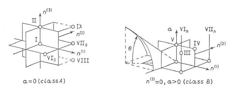
Figure 1: The parameter space ${\cal C}_{D}$ as a 3-plane (class A) and an orthogonal half 3-plane (class B) in $R^{4}$ with coordinates $(n^{(1)},n^{(2)},n^{(3)},a)$, showing the canonical representatives of each Bianchi type. Of the 8 open octants in the class A case, 2 and 6 respectively represent type IX and VIII, while half of the 12 open faces bounding these octants represent type VII₀ and the other half type VI₀; the 6 coordinate open half lines represent type II and the origin type I. Similarly in the class B case, half of the 4 open octants are associated with each of the 1-parameter family of Bianchi types VI_h and VII_h, a single isomorphism class corresponding to a constant value surface of the function $h=a^{2}(n^{(1)}n^{(2)})^{-1}$. A typical such surface is illustrated in one octant, the angle $\theta$ given by $\tan\theta=|h/2|^{1/2}$; those in the remaining octants are obtained by rotation through multiples of $\pi/2$, $h$ alternating in sign for a given magnitude $|h|$. The 4 vertical open faces bounding these octants all represent type IV and the positive $a$-axis type V, with the $a=0$ plane giving the class A limit of each type.

The space ${\cal C}_{D}$ is very useful in describing the notion of Lie algebra contraction [50]. Consider the effect on ${\cal C}_{D}$ of an arbitrary positive-definite diagonal matrix transformation, i.e. an element of the 3-dimensional abelian “scale group” $Diag(3,R)^{+}$ (the identity component of the diagonal subgroup $Diag(3,R)$ of $GL(3,R)$ whose Lie algebra $diag(3,R)$ consists of the diagonal elements of $gl(3,R)$ ) which represents independent scalings of the standard basis vectors of $R^{3}$ or of the basis vectors of any 3-dimensional vector space. Such a matrix may be represented in the form

 

$${e^{{\kern-0.17496pt\hbox{$\beta$}\kern-3.95938pt\kern 0.35002pt\hbox{$\beta$}\kern-3.95938pt\kern-0.17496pt\raise 0.30313pt\hbox{$\beta$}}}}$$

 

and its left action on ${\cal C}_{D}$ via (2.5) is

$$\overline{n}^{(a)}=j_{\hbox{$e^{{\kern-0.12247pt\hbox{$\beta$}\kern-2.77156pt\kern 0.24501pt\hbox{$\beta$}\kern-2.77156pt\kern-0.12247pt\raise 0.21219pt\hbox{$\beta$}}}$}}(n^{(a)})=e^{2\beta^{a}-(\beta^{1}+\beta^{2}+\beta^{3})}n^{(a)}\quad,\qquad\overline{a}=j_{\hbox{$e^{{\kern-0.12247pt\hbox{$\beta$}\kern-2.77156pt\kern 0.24501pt\hbox{$\beta$}\kern-2.77156pt\kern-0.12247pt\raise 0.21219pt\hbox{$\beta$}}}$}}(a)=e^{-\beta^{3}}a\ .$$

The barred components represent another point in the same orbit as long as the scale transformation is nonsingular. However, if one takes a singular limit a point on the boundary of an orbit can be reached resulting in a change of Bianchi type. This is called Lie algebra contraction [50].

When a given stratum consists of a family of orbits as is the case for types VI_h≤0 and VII_h≥0, in order to arrive at a point of the boundary of a given stratum not at the boundary of the starting orbit, one must allow motion transversal to the orbits; such a motion is called a Lie algebra deformation. For these two Bianchi types, changing the parameter $h$ represents a Lie algebra deformation. For example, a type IV or V point of ${\cal C}_{D}$ can be reached from a type VI_h≠0 or type VII_h≠0 point only by a deformation.

Table 2: The “reduced” specialization diagram describing the possible Lie algebra contractions and deformations of the Bianchi types and their orbit dimensions restricted to the standard diagonal form subspace ${\cal C}_{D}$ of the space ${\cal C}$ of possible structure constant tensors. Not shown are direct paths between Bianchi types which may be connected through other Bianchi types by the indirect paths shown. The final column indicates the identity component of the canonical special automorphism matrix group of each type, with notation explained in appendix B.

Apart from trivial permutations, each of the canonical points of ${\cal C}_{D}$ may undergo such Lie algebra contractions and/or deformations to arrive at canonical points lying in the same stratum or in lower-dimensional strata at the boundary of the given stratum. The various possibilities are illustrated in Table 2 following MacCallum [39]. Each class B Bianchi type has a corresponding class A limit obtained by the contraction (V, IV) or deformation (VI_h, VII_h) $\quad a\to 0$ shown in Table 2. (Unfortunately the type II components arising from this contraction of the canonical type IV components differ from the canonical type II components by a permutation.) By extending the scale group to the complex domain, one may perform a rotation in the complex plane which directly connects the canonical components of certain Bianchi types. For example, the scaling $\hbox{diag}(e^{i\theta},e^{i\theta},1)$ with $\theta\in[0,{\pi\over 2}]$ is a path connecting the canonical components of types VIII and IX, which represent inequivalent real forms of the same complex Lie algebra. The types VII_h≠0 and VII_h≠0 also require analytic continuation of the parameter $a$ as well. Such pairs are connected by horizontal dotted lines in Table 2.

If the real scaling matrix $e^{\kern-0.12251pt\hbox{$\scriptstyle\beta$}\kern-2.77156pt\kern 0.24503pt\hbox{$\scriptstyle\beta$}\kern-2.77156pt\kern-0.12251pt\raise 0.21213pt\hbox{$\scriptstyle\beta$}}$ is highly anisotropic, i.e. “nearly singular”, its action on a canonical point of ${\cal C}_{D}$ may simulate a Lie algebra contraction on the space of functions on ${\cal C}_{D}$: the value of a function of the structure constant tensor components at the image point will approximately equal its value at the nearest point of the boundary. Thus under very anisotropic scalings, functions of a given Bianchi type structure constant tensor approach those of a contracted type. This is a very useful way of viewing the behavior of highly anisotropic Bianchi cosmologies, as will be described below.

Equations (2.10) represent a ${\cal C}_{D}$-parametrized Lie algebra $g_{{}_{{\cal C}_{D}}}$ . Using a trick involving the linear adjoint group, one may realize this Lie algebra as the Lie algebra of left invariant vector fields on a ${\cal C}_{D}$-parametrized simply connected Lie group $G_{{}_{{\cal C}_{D}}}$, where the parametrization arises by introducing canonical coordinates of the second kind with respect to the basis $e_{{}_{{\cal C}_{D}}}$ of $g_{{}_{{\cal C}_{D}}}$ whose brackets are given by (2.10). These coordinates have range $R^{3}$ and are global for all Bianchi types but type IX where the simply connected group manifold is instead $S^{3}$ and these coordinates form a local patch centered at the identity. These results are summarized in appendix A and illustrate the elegant consequences of the first diagonalization referred to in the introduction.

The result of this long digression is the ${\cal C}_{D}$-parametrized simply connected Lie group $G_{{}_{{\cal C}_{D}}}$ which enables one to simultaneously describe all 3-dimensional (simply connected) Lie groups. One may next introduce the ${\cal C}_{D}$-parametrized left invariant Riemannian 3-manifold ($G_{{}_{{\cal C}_{D}}},\hbox{\sl g}_{{}_{{\cal C}_{D}}}$) or “homogeneous Riemannian 3-space” with metric

$$\hbox{\sl g}_{{}_{{\cal C}_{D}}}=g_{ab}\ \omega^{a}_{{}_{{\cal C}_{D}}}\otimes\omega^{b}_{{}_{{\cal C}_{D}}}\ ,$$

where $e_{{}_{{\cal C}_{D}}}$ and $\{\omega^{a}_{{}_{{\cal C}_{D}}}\}$ are the explicit ${\cal C}_{D}$-parametrized fields given by formulas (A.9) and the component matrix $\hbox{\bf g}=(g_{ab})=g_{ab}\hbox{\bf e}^{b}{}_{a}$ with determinant $g=\det\hbox{\bf g}$ lies in the 6-dimensional space ${\cal M}\subset GL(3,R)$ of component matrices of positive-definite inner products on $R^{3}$. This space, through (2.13), parametrizes the space ${\cal M}_{L}(G_{{}_{{\cal C}_{D}}})$ of left invariant metrics on the Lie group $G_{{}_{{\cal C}_{D}}}$. Since it is a bit awkward, the subscript ${\cal C}_{D}$ will usually be omitted in what follows. Before moving on to the ${\cal C}_{D}$-parametrized spatially homogeneous spacetime, it pays to examine the curvature of the ${\cal C}_{D}$-parametrized homogeneous Riemannian 3-space and the isometry classes of the space of such Riemannian manifolds. The latter question leads to the second diagonalization mentioned in the introduction.

The isometry classes of ${\cal M}_{L}(G)$ are its intersections with the orbits of the diffeomorphism group ${\cal D}(G)$ on the space of all smooth Riemannian metrics on $G$. Consider instead the largest subgroup of ${\cal D}(G)$ which acts on the space ${\cal M}_{L}(G)$, i.e. which maps all left invariant metrics into left invariant metrics under the dragging along action. This is possible only if it maps the Lie algebra $g$ into itself and hence the space of all left invariant tensor fields into itself under dragging along. The orbits of this group on ${\cal M}_{L}(G)$ should correspond to the isometry classes of left invariant metrics; it is assumed that they do.

The “symmetry compatible subgroup” of ${\cal D}(G)$ having this property, already designated by ${\cal D}(g)$ earlier in this section, is the semidirect product Lie group of translations and automorphisms of $G^{\ \ (1)}$

$${\cal D}(g)=L_{G}\times_{s}Aut(G)=R_{G}\times_{s}Aut(G)\ .$$

The equality of the two semidirect products is connected with the adjoint group $\ AD_{G}\ \subset$ $Aut(G)$ of $G$, also called the group of inner automorphisms of $G$. In addition to the effective left action of any Lie group $G$ on itself by left translation $L$ and inverse right translation $R^{-1}$ which are commuting actions due to the associativity of the group multiplication, $G$ may act on itself on the left by inner automorphism: $AD_{a}=L_{a}\circ R^{-1}_{a}=R^{-1}_{a}\circ L_{a}$. The image group $AD_{G}$ is a homomorphic subgroup of the automorphism group of $G$ but is not necessarily isomorphic to $G$. They are isomorphic and the adjoint action effective when $AD_{a_{0}}$ is the only transformation acting as the identity, i.e. when the center $C(G)=\{a\in G\bigm{|}AD_{a}=Id\}$ of $G$ is trivial (contains only the identity $a_{0}$). Returning to (2.l4), the fact that $AD^{-1}_{a}\circ\alpha\in Aut(G)$ if $\alpha\in Aut(G)$ together with the identity $L_{a}\circ\alpha=R_{a}\circ(AD^{-1}_{a}\circ\alpha)$ explains the equality of the two semidirect products.

This discussion may be repeated at the Lie algebra level for the Lie algebra $\hbox{\hbox to0.0pt{\hskip 1.5pt\raise 0.75pt\hbox{--}\hss}${\cal X}$}(g)$ which generates ${\cal D}(g)$, a semidirect sum Lie subalgebra of the Lie algebra $\hbox{\hbox to0.0pt{\hskip 1.5pt\raise 0.75pt\hbox{--}\hss}${\cal X}$}(G)$ of smooth vector fields on $G$

$$\hbox{\hbox to0.0pt{\hskip 1.5pt\raise 0.75pt\hbox{--}\hss}${\cal X}$}(g)=\tilde{g}\oplus_{s}\,aut(G)=g\oplus_{s}aut(G)\ .$$

Here $aut(G)$ generates $Aut(G)$ and ${\rm ad}(G)=g-\tilde{g}\equiv\{X^{a}(e_{a}-\tilde{e}_{a})\bigm{|}(X^{a})\in R^{3}\}$ generates the adjoint group.

When the group ${\cal D}(g)$ acts on $g$ by dragging along, $L_{G}$ has no action by definition, while $R_{G}$ and $AD_{G}$ have the same action, inducing inner automorphisms of the Lie algebra: $R^{-1}_{a}X=AD_{a}X\equiv Ad(a)X\in g$ for $X\in g$. The image subgroup $Ad(G)$ of the general linear group of $g$ is called the linear adjoint group and when $G$ is connected coincides with the group $IAut(g)\subset Aut(g)$ of inner automorphisms of $g$ ; its matrix representation $Ad_{e}(g)$ with respect to a basis $e$ of $g$ is exploited in appendix A. Similarly by dragging along, $Aut(G)$ induces the action on $g$ of the full group $Aut(g)$ of automorphisms of $g$ when $G$ is simply connected as is assumed here. Left invariant tensor fields undergo the transformation associated with the corresponding tensor representation of this group. Similarly when $\hbox{\hbox to0.0pt{\hskip 1.5pt\raise 0.75pt\hbox{--}\hss}${\cal X}$}(g)$ acts on $g$ by Lie derivation (define ${\rm ad}(\xi)X=\hbox{\it\char 36\relax}_{\xi}X$ for $\xi\in\hbox{\hbox to0.0pt{\hskip 1.5pt\raise 0.75pt\hbox{--}\hss}${\cal X}$}(g)$ and $X\in g$ and let ${\rm ad}_{e}(\xi)$ be the matrix of ${\rm ad}(\xi)$ with respect to the basis $e$ of $g$), $\tilde{g}$ has no effect, while $g$ and ${\rm ad}(G)$ have the same action, inducing inner derivations of $g$ (the image Lie subalgebra $\hbox{ad}(g)\subset aut(g)$), while $aut(g)$ induces the action of the full Lie algebra of derivations $der(g)=aut(g)$ of $g$, with matrix representation $aut_{e}(g)$. The Lie algebra $aut(g)$ generates the automorphisms of $g$ .

Thus when ${\cal D}(g)$ acts on the left invariant metric (2.13) by dragging along, the component matrix g undergoes the appropriate transformation law associated with the matrix automorphism group. If $\hbox{\bf A}\in Aut_{e}(g)$ is an induced matrix automorphism of $g$ , this transformation law is

$$\hbox{\bf g}\in{\cal M}\qquad\to\qquad f_{\hbox{\bf A}}(\hbox{\bf g})=\hbox{\bf A}^{-1T}\hbox{\bf g}\hbox{\bf A}^{-1}\ .$$

The orbits of this action of $Aut_{e}(g)$ on ${\cal M}$ through the correspondence (2.13) represent the isometry classes of left invariant metrics. However, just as the space ${\cal C}$ could be reduced to its essential structure by diagonalization, here too the “offdiagonal” metric matrix variables are superfluous and all the essential information is carried by the diagonal submanifold ${\cal M}_{D}$ of ${\cal M}$, assuming that $e$ is a basis of $g$ whose structure constant tensor components belong to ${\cal C}_{D}$. This submanifold ${\cal M}_{D}$, like the space ${\cal C}_{D}$, is also a “slice” for the natural action of the orthogonal group on the full space. (The reduction of ${\cal M}\times{\cal C}$ to ${\cal M}_{D}\times{\cal C}_{D}$ is a consequence of the well known fact that one can always simultaneously diagonalize two real symmetric matrices by an orthogonal transformation.) In fact ${\cal M}_{D}$ is a “slice” for the action (2.16) of any 3-dimensional subgroup ${\hat{G}}\subset GL(3,R)$ whose matrix Lie algebra $\hat{g}$ has a basis $\{\kern-0.24994pt\hbox{$\kappa$}\kern-5.76158pt\kern 0.50003pt\hbox{$\kappa$}\kern-5.76158pt\kern-0.24994pt\raise 0.43304pt\hbox{$\kappa$}_{a}\}$ with the following property: for each cyclic permutation $(a,b,c)$ of $(1,2,3)$, the matrix $\kern-0.24994pt\hbox{$\kappa$}\kern-5.76158pt\kern 0.50003pt\hbox{$\kappa$}\kern-5.76158pt\kern-0.24994pt\raise 0.43304pt\hbox{$\kappa$}_{a}$ belongs to $\hbox{span}\ \{\hbox{\bf e}^{b}{}_{c},\hbox{\bf e}^{c}{}_{\ b}\}$, where $\{\hbox{\bf e}^{a}{}_{b}\}$ is the natural basis of $gl(3,R)$ already introduced above. In appendix B, the matrix automorphism group is described for the ${\cal C}_{D}$-parametrized Lie algebra $g$ . It always contains such a subgroup $\hat{G}$, which may be used to map a general point of ${\cal M}$ to the diagonal submanifold ${\cal M}_{D}$. It therefore suffices to consider those automorphisms which map ${\cal M}_{D}$ into itself to determine the isometry classes. Since ${\cal M}_{D}$ is mapped into itself by all permutations and diagonal transformations, it suffices to consider elements of $Aut_{e}(g)$ of this type.

${\cal M}_{D}$ consists of all diagonal matrices with positive entries and clearly coincides with the scale group $Diag(3,R)^{+}$ as a submanifold of $GL(3,R)$ . They are best identified, however, in terms of the simply transitive action of $Diag(3,R)^{+}$ on ${\cal M}_{D}$ using the identity matrix $\hbox{\bf 1}\in{\cal M}_{D}$ as a reference point, as described at the beginning of this section. The abelian group $Diag(3,R)^{+}$ is most naturally parametrized by its Lie algebra $diag(3,R)$ which in turn parametrizes ${\cal M}_{D}$

$$\kern-0.24994pt\hbox{$\beta$}\kern-5.65625pt\kern 0.50003pt\hbox{$\beta$}\kern-5.65625pt\kern-0.24994pt\raise 0.43304pt\hbox{$\beta$}=\hbox{diag}(\beta^{1},\beta^{2},\beta^{3})\ ,\hfil$$

The prime on $\hbox{\bf g}^{\prime}$ serves as a reminder of its diagonality, while the right action $f^{-1}$ is used to conform with convention. Through (2.17) the single matrix $\beta$$\beta$$\beta$ simultaneously represents three different diagonal matrices. The special scale group $SDiag(3,R)^{+}=Diag(3,R)^{+}\cap SL(3,R)$ with Lie algebra $sdiag(3,R)=\{\kern-0.24994pt\hbox{$\beta$}\kern-5.65625pt\kern 0.50003pt\hbox{$\beta$}\kern-5.65625pt\kern-0.24994pt\raise 0.43304pt\hbox{$\beta$}\in diag(3,R)\bigm{|}\hbox{Tr}\ \kern-0.24994pt\hbox{$\beta$}\kern-5.65625pt\kern 0.50003pt\hbox{$\beta$}\kern-5.65625pt\kern-0.24994pt\raise 0.43304pt\hbox{$\beta$}=0\}$ is related in a similar way to the unimodular submanifold $\overline{{\cal M}}_{D}={\cal M}_{D}\cap SL(3,R)$; the following notation proves convenient

 

$$\beta$$

 

Misner [15] introduced a basis of $diag(3,R)$ and $sdiag(3,R)$ which is orthonormal with respect to the inner product $\left<\left<,\right>\right>_{{}_{DW}}={1\over 6}\left<,\right>_{{}_{DW}}$ on $gl(3,R)$, where the DeWitt inner product and trace inner product on $gl(3,R)$ are defined by

 

$${\left<\hbox{\bf A},\hbox{\bf B}\right>_{{}_{DW}}}$$

 

This basis and the corresponding parametrization of $diag(3,R)$ and $sdiag(3,R)$ are given by

 

$$\beta$$

 

These may be generalized by the definitions

 

$${\beta^{+}_{a}}$$

 

with $\beta^{\pm}=\beta^{\pm}_{3}$ and the others obtained by cyclic permutation of indices. For each cyclic permutation $(a,b,c)$ of $(1,2,3)$, the Taub submanifold ${\cal M}_{T(a)}=\{\hbox{\bf g}^{\prime}\in{\cal M}_{D}\bigm{|}g^{\prime}_{bb}=g^{\prime}_{cc}\}$ and its unimodular submanifold $\overline{{\cal M}}_{T(a)}\subset\overline{{\cal M}}_{D}$ may be equivalently defined by $\beta^{bc}=0$ or $\beta^{-}_{a}=0$. They intersect at the isotropic submanifold ${\cal M}_{I}$ and $\overline{{\cal M}}_{I}=\{\hbox{\bf 1}\}$ respectively, for which $\beta^{+}=\beta^{-}=0$. Since $\hbox{\bf g}^{\prime}=e^{2\beta^{0}}e^{2\hat{{\kern-0.17496pt\hbox{$\beta$}\kern-3.95938pt\kern 0.35002pt\hbox{$\beta$}\kern-3.95938pt\kern-0.17496pt\raise 0.30313pt\hbox{$\beta$}}}}$, translation along $\beta^{0}$ represents a conformal rescaling of the metric (2.13) under which all curvatures scale by a factor $e^{q\beta^{0}}$ where q is an appropriate dimension. Thus the nontrivial information about curvature is associated with the conformal submanifold $\overline{{\cal M}}_{D}$  (namely $\beta^{0}=0$).

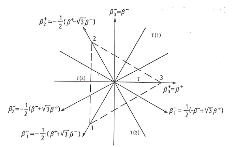
Figure 2: The $\beta^{+}\beta^{-}$ plane: $sdiag(3,R)\sim SDiag(3,R)^{+}\sim\overline{{\cal M}}_{D}$. Shown are the three pairs of orthogonal axes related by rotations of angle $2\pi/3$. The $\beta^{+}_{a}$-axis is the projection of the Taub submanifold ${\cal M}_{T(a)}$ to $\overline{{\cal M}}_{D}$, while the origin represents the projection of the isotropic submanifold ${\cal M}_{I}$. Lines parallel to the sides of the triangle are associated with constant values of the three diagonal components of the conformal metric matrix while lines parallel to the bisectors of the vertex angles are associated with constant values of their ratios. Reflections and permutations of the basis $e$ act on $\overline{{\cal M}}_{D}$ as the symmetry group of the equilateral triangle of this figure.

The $\beta^{+}\beta^{-}$ plane, i.e. $sdiag(3,R)\sim SDiag(3,R)\sim\overline{{\cal M}}_{D}$ is illustrated in Figure 2, indicating the Taub and isotropic submanifolds and each of the pairs of coordinate axes associated with the three coordinate systems $\{\beta^{+}_{a},\beta^{-}_{a}\}$. Each pair of coordinate vectors, namely $\{\hbox{\bf e}_{a+},\hbox{\bf e}_{a-}\}$, is orthonormal with respect to the inner product $\langle\langle,\rangle\rangle$. Interpreting the $\beta^{+}\beta^{-}$ plane as $\overline{{\cal M}}_{D}$, a cyclic permutation of the basis $e$ of $g$ leads through (2.13) and (2.16) to a rotation of the coordinate axes by $\pm 2\pi/3$, while a transposition of two basis elements, say $e_{b}$ and $e_{c}$, leads to a reflection about the Taub submanifold $\overline{{\cal M}}_{T(a)}$, where (a,b,c) is a cyclic permutation of $(1,2,3)$ . The action of the discrete group of permutations on $\overline{{\cal M}}_{D}$ thus coincides with the symmetry group of the equilateral triangle shown in Figure 2, whose sides are parallel to the constant value lines of the $\beta^{+}_{a}$-coordinates and whose orthogonal bisectors are the Taub submanifolds. (Note that rotations about one of the frame vectors by $\pm\pi/2$ have the same effect on the $\beta^{+}\beta^{-}$ plane as transpositions.) The translations of the $\beta^{+}\beta^{-}$ plane correspond to the action on $\overline{{\cal M}}_{D}$ of the special scale group.

The Lie algebra contractions of the space ${\cal C}_{D}$ arising from singular limits of the action of the scale group on this space are now easily described. Let $\{\beta=s\hbox{\bf b}\bigm{|}s\in(-\infty,0]\}$ be a ray from the origin of $diag(3,R)$ parametrized by $s$ and extend all of the subscript and superscript notation of (2.17)-(2.21) to the constant diagonal matrix b ; then (2.12) becomes

$$j^{-1}_{\hbox{$e^{{\kern-0.12247pt\hbox{$\beta$}\kern-2.77156pt\kern 0.24501pt\hbox{$\beta$}\kern-2.77156pt\kern-0.12247pt\raise 0.21219pt\hbox{$\beta$}}}$}}(n^{(a)},a)=(e^{s(b^{0}+4b^{+}_{a})}n^{(a)},e^{s(b^{0}-2b^{+}_{3})}a)\ .$$

If $b^{0}\neq 0$, then one might as well set $b^{0}=1$. In order that this have a finite limit as $s=\beta^{0}\to-\infty$ leading to a singular scale transformation $(\det e^{\kern-0.12251pt\hbox{$\scriptstyle\beta$}\kern-2.77156pt\kern 0.24503pt\hbox{$\scriptstyle\beta$}\kern-2.77156pt\kern-0.12251pt\raise 0.21213pt\hbox{$\scriptstyle\beta$}}=e^{3\beta^{0}}\to 0)$ which therefore induces a Lie algebra contraction, the following inequalities must be satisfied when the corresponding structure constant tensor component is nonvanishing

$$n^{(a)}\neq 0:\quad b^{+}_{a}\geq-{1\over 4};\qquad a\neq 0:\quad b^{+}_{3}\leq{\textstyle{1\over 2}}\ .$$

These inequalities are illustrated in Figure 3. The label of a given dashed line indicates the structure constant tensor component which remains fixed under the scaling (2.23) associated with the points of the line, all points to the origin side of the line leading to a limit where that structure constant tensor component goes to zero and all points to the other side not leading to a finite limit if that component is nonzero. Thus all points in the interior of the triangle 123 lead to the abelian limit $(0,0,0,0)$, vertex 1: $(0,n^{(2)},n^{(3)},0)$, vertex 2: $(n^{(1)},0,n^{(3)},0)$, vertex 3: $(n^{(1)},n^{(2)},0,a)$, open side 23: $(n^{(1)},0,0,0)$, open side 31: $(0,n^{(2)},0,0)$ and open side 12: $(0,0,n^{(3)},0)$.

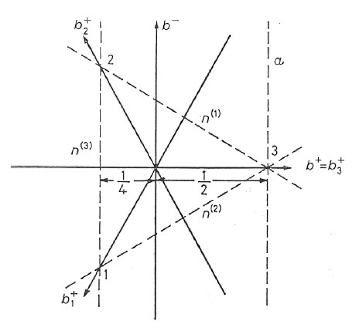
Figure 3: The parameter space for the family of Lie algebra contractions of the space ${\cal C}_{D}$.

On the other hand when $b^{0}=0$, at least one of the components of $e^{\kern-0.12251pt\hbox{$\scriptstyle\beta$}\kern-2.77156pt\kern 0.24503pt\hbox{$\scriptstyle\beta$}\kern-2.77156pt\kern-0.12251pt\raise 0.21213pt\hbox{$\scriptstyle\beta$}}$ must go to infinity as $s\to-\infty$ so a finite limit can result only if one of the components of n is zero. If $(a,b,c)$ is a cyclic permutation of (1,2,3) and $n^{(a)}=0$, then the limit $s\to-\infty$ of (2.22) will be finite only if $b^{+}_{b}\geq 0$ and $b^{+}_{c}\geq 0$, which is the sector of the plane between the positive $b^{+}_{c}$ and $b^{+}_{c}$ axes, the limit being (0,0,0,0) between the axes, but with $j_{\hbox{$e^{{\kern-0.12247pt\hbox{$\beta$}\kern-2.77156pt\kern 0.24501pt\hbox{$\beta$}\kern-2.77156pt\kern-0.12247pt\raise 0.21219pt\hbox{$\beta$}}}$}}(n^{(b)},n^{(c)},a)$ having the limit $(n^{(b)},0,0)$ on the $b^{+}_{b}$-axis and $(0,n^{(c)},0)$ on the $b^{+}_{c}$-axis. This class of Lie algebra contractions might be called “pure anisotropy” contractions.

Returning now to the question of isomorphism classes within the diagonal submanifold ${\cal M}_{D}$, namely the orbits of the action of the diagonal and permutation automorphisms on ${\cal M}_{D}$, one has four different cases corresponding to the four categories of Table 2. Modulo discrete automorphisms, the diagonal automorphisms of the ${\cal C}_{D}$-parametrized Lie algebra are described for each of these categories in Appendix B. For the first category only permutation and reflection automorphisms act on ${\cal M}_{D}$ so ${\cal M}_{D}$ itself locally parametrizes the space of automorphism group orbits on ${\cal M}$. (For the canonical type IX case the six sectors into which the three $\beta^{+}_{a}$ axes divide the $\beta^{+}\beta^{-}$ plane are all isometric for a given value of $\beta^{0}$, but in the canonical type VIII case only reflection about $\overline{{\cal M}}_{T(3)}$ connects isometric points.) For the second category of Table 2, there exists a diagonal automorphism subgroup generated by the matrix $\hbox{\bf I}^{(3)}=\hbox{diag}(1,1,0)$ when $n^{(3)}=0$, leading to translations along $\beta^{+}=\beta^{+}_{3}$ in the $\beta^{+}\beta^{-}$ plane, so $\beta^{-}=\beta^{-}_{3}$ together with $\beta^{0}$ locally parametrize the orbit space. The result for the other components $(n^{(3)}\neq 0)$ of ${\cal C}_{D}$ belonging to this category may be obtained by cyclic permutation. For the third category automorphisms induce translations along both $\beta^{+}$ and $\beta^{-}$ so all points of the $\beta^{+}\beta^{-}$ plane are equivalent and $\beta^{0}$ alone parametrizes the orbit space, while in the abelian case ${\cal M}$ consists of a single orbit.

For the upper two categories of Table 2, the generic points of ${\cal M}_{D}$ belong to an orbit on ${\cal M}$ having three dimensions transversal to ${\cal M}_{D}$ and at most a discrete isotropy group. However, on certain submanifolds of ${\cal M}_{D}$ and for certain Bianchi types the full orbit dimension decreases and only one or no directions remain transversal to ${\cal M}_{D}$. At these points the isotropy group has dimension greater than zero corresponding to additional symmetries of the metric (2.13). This occurs at the Taub submanifold ${\cal M}_{T(a)}$ when $n^{(b)}=n^{(c)}$ ($(a,b,c)$ is a cyclic permutation of $(1,2,3)$) corresponding to local rotational symmetry (necessarily the index $a=3$ in the class B case) and at the isotropic submanifold ${\cal M}_{I}$ when $n^{(1)}=n^{(2)}=n^{(3)}$ corresponding to isotropy. For the lower two categories the isotropy group has generic dimension greater than zero so there are always additional symmetries. However, the Taub submanifolds are still relevant to spacetime symmetries. The choice of canonical components for Bianchi type II was made so that ${\cal M}_{T(3)}$ is associated with additional spacetime symmetry for all canonical points of ${\cal C}_{D}$. This is discussed in greater detail elsewhere [43]. For the noncanonical points of ${\cal C}_{D}$ the submanifolds relevant to additional symmetry change as described below.

The discussion of isometry classes and additional symmetries is not just an interesting aside, but is important for appreciating the symmetries of the scalar curvature $R$ of the metric (2.13). This function on ${\cal M}\times{\cal C}_{D}$ is a scalar under a change of basis $e$ of $g$ and hence is invariant under the action of the matrix automorphism group on ${\cal M}$ alone, having a constant value on each orbit. Using standard formulas one may easily evaluate the components of the connection of the metric (2.13), raising and lowering all indices with the component matrices g and g^-1

$$\nabla_{\hbox{$e_{a}$}}e_{b}={\mit\Gamma}^{c}{}_{ab}e_{c}\ ,\quad{\mit\Gamma}^{c}{}_{ab}={\textstyle{1\over 2}}C^{c}{}_{ab}+C_{(a\hskip 5.0ptb)}^{\hskip 7.0ptc}\ .$$

Introducing the unit alternating (pseudo-)tensor $\eta_{abc}=g^{1\over 2}\epsilon_{abc}$ and the two matrices $\hbox{\bf m}=g^{-{1\over 2}}\hbox{\bf ng}$ and $A=a_{c}\eta^{ca}_{\hskip 6.0ptb}\hbox{\bf e}^{b}{}_{a}$, the Ricci tensor and scalar curvature of this connection are then found to have the following expressions

 

R $${{}=R^{a}{}_{b}\hbox{\bf e}^{b}{}_{a}=2\hbox{\bf m}^{2}-\hbox{\bf m}\hbox{Tr}\ \hbox{\bf m}-\hbox{\bf 1}(\hbox{Tr}\ \hbox{\bf m}^{2}-{\textstyle{1\over 2}}\hbox{Tr}^{2}\hbox{\bf m}+2a_{c}a^{c})+[\hbox{\bf m,A}]}$$

 

where the conventions of Misner, Thorne and Wheeler [18] are followed for curvature tensor definitions. Assuming as always that $C^{a}{}_{bc}\in{\cal C}_{D}$, these are ${\cal C}_{D}$-parametrized functions on ${\cal M}$. Note that for $\hbox{\bf g}\in{\cal M}_{D}$ the Ricci tensor component matrix is diagonal except for the last term which contributes a 12 (and 21) component in the class B case. In the class A case $e$ is then an orthogonal frame of Ricci eigenvectors, while linear combinations of $e_{1}$ and $e_{2}$ must be taken to obtain such a frame in the class B case, leading to structure constant tensor components not belonging to ${\cal C}_{D}$.

One may also introduce a potential function and several 1-forms on ${\cal M}$ which may be interpreted as force fields

 

$${U_{G}}$$

 

The scalar curvature potential function $U_{G}$ serves as a potential for the Einstein force field $G$ in the class A case where $Q$ vanishes, but in the class B case the Einstein force field has a nonpotential component $Q$ which generically satisfies $Q\neq 0\neq dQ$. As a ${\cal C}_{D}$-parametrized function on ${\cal M}_{D}$, the scalar curvature potential is given explicitly by

$$\hfil U_{G}$$

The values of the curvature function $V^{\ast}$ (a scalar density of weight $2\over 3$ which may be expressed in the form $V^{\ast}=g^{-{1\over 6}}{\cal G}^{-1}_{abcd}n^{ab}n^{cd}$ using (2.40)) at the canonical points of ${\cal C}_{D}$ are

IX/VIII: $$2e^{4\beta^{+}}\hbox{sinh}^{2}2\sqrt{3}\beta^{-}\mp 2e^{-2\beta^{+}}\hbox{cosh}\ 2\sqrt{3}\beta^{-}+{\textstyle{1\over 2}}e^{-8\beta^{+}}\hfil$$

VII:

II:

I,V:

Suppose $Y$ is a function on ${\cal M}\times{\cal C}$ which is a scalar under a change of basis $e$ of $g$ and therefore satisfies $Y(\hbox{\bf g},C^{a}{}_{bc})=Y(f_{\hbox{\bf A}}(\hbox{\bf g}),j_{\hbox{\bf A}}(C^{a}{}_{bc}))$ or equivalently $Y(f_{\hbox{\bf A}}^{-1}(\hbox{\bf g}),C^{a}{}_{bc})=Y(\hbox{\bf g},j_{\hbox{\bf A}}(C^{a}{}_{bc}))$. Focussing now on ${\cal M}_{D}\times{\cal C}_{D}$ and letting $j_{\hbox{\bf A}}$ be one of the Lie algebra contractions (2.22)-(2.23), one sees that the effect on the function $Y$ of such a contraction is equivalent to an infinite translation of ${\cal M}_{D}\sim diag(3,R)\sim R^{3}$. The value of the function for the original point $C^{a}{}_{bc}$ therefore approaches its value for the contracted points as one approaches infinity in ${\cal M}_{D}\sim diag(3,R)\sim R^{3}$ in the negative $\beta^{0}$ direction. $e^{-2\beta^{0}}V^{\ast}$ is such a scalar function and hence as one approaches infinity in the $\beta^{+}\beta^{-}$ plane along the directions parametrized in Figure 3, the density $V^{\ast}$ approaches a rescaled version of the potential of the corresponding contracted points of ${\cal C}_{D}$. Furthermore the difference between $V^{\ast}$ and its contracted value at the same point of the $\beta^{+}\beta^{-}$ plane as one gets far from the origin becomes very small compared to the value itself.

Figure 4: Suggestive contours of the potential function $V^{\ast}$ on the $\beta^{+}\beta^{-}$ plane are shown for the canonical points of ${\cal C}_{D}$ (not shown is the type IV case which is related to type II by an active rotation of $4\pi/3$) and values of $V^{\ast}$ are plotted for the Taub submanifold $\overline{{\cal M}}_{T(3)}$, namely the $\beta^{+}$-axis. Unit distances are marked on the coordinate axes. Arrows indicate the direction of the associated force field, pointing toward directions along which the potential decreases. Note that $V^{\ast}$ is nonnegative except in the type IX case where the contours are closed for $V^{\ast}<0$ and open for $V^{\ast}\geq 0$, the minimum value -1.5 occurring at the origin or isotropic submanifold $\overline{{\cal M}}_{I}$.

This can be seen in the diagrams of Figure 4 which show suggestive contours of the potential $V^{\ast}$ for canonical points of ${\cal C}_{D}$. Contours of the same five function values are shown for each type, together with two additional closed contours for the type IX region where $V^{\ast}$ is negative. As one proceeds along any of the positive $\beta^{+}_{a}$ axes in the type IX case or the $\beta^{+}$ axis in the type VIII case, the potential quickly approaches that of a permutation of the canonical type VII potential, while along the positive $\beta^{+}_{1}$ and $\beta^{+}_{2}$ axes the type VIII potential approaches a permutation of the type VI potential. For directions in between these three positive axes the potential quickly approaches that of a permutation of the type II potential. Similarly the type VII and VI potentials approach permutations of the type II potential for directions between the positive $\beta^{+}$ and $\beta^{+}_{1}$ axes and the positive $\beta^{+}$ and $\beta^{+}_{2}$ axes, but type I in the remaining sector. Finally the type II potential approaches type I along all directions in the positive $\beta^{+}$ half plane. Note further that for all the nonsemisimple types the potential $V^{\ast}$ simply scales under translation along $\beta^{+}$, so the contours are simply translates of each other, a consequence of the existence of the additional diagonal automorphism generated by the matrix $\hbox{\bf I}^{(3)}\equiv\hbox{diag}(1,1,0)$, except for type II where the matrix is instead diag$(1,1,2)$. The reflection and permutation symmetries of all of the potentials reflect the existence of discrete symmetries. The reflection symmetry about the $\beta^{+}$ axis for all types but IV is connected with a discrete automorphism whose existence motivated the choice of canonical type II components.

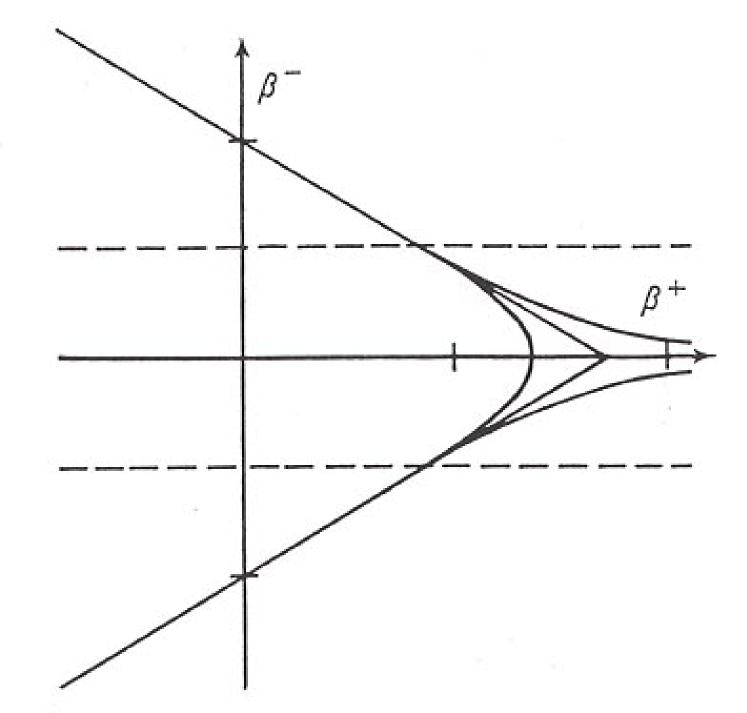
Figure 5: Open and closed channel contours and their asymptotes.

The dashed straight lines in Figure 4 indicate “channels” of width 1 outside of which the contours are essentially the same as the corresponding asymptotic Bianchi type II potential (the difference becoming exponentially small with distance from the origin). These channels themselves are either open or closed; outside of the dashed circles of diameter 1 in the type IX and type VIII figures, the open and closed channels are essentially the same of the corresponding type VII and VI channels respectively, where these latter channels are rotated by $\pm{2\pi/3}$ for comparison. (Corresponding contours are separated by a distance of less that .01 as one exits the circle and the difference decreases exponentially with distance from the origin.) Figure 5 shows the type VII and VI contours of the same function value together with the asymptotic type II contours of the same function value, showing that the deviation of the open and closed channel contours from the type II asymptotes only becomes important within the channel itself. The only region of the type IX and VIII potentials which is essentially different from those of the remaining Bianchi types (arising from them by contraction) is the interior of the dashed circle which occurs at the intersections of the three channels; similarly only the channels of the type VII and VI potentials are different from the potentials of the contracted types I and II.

The potentials for the noncanonical points of ${\cal C}_{D}$ are obtained merely by translating the origin of coordinates in the $\beta^{+}\beta^{-}$ plane and rescaling the potential. Let $C^{a}{}_{bc}(can)\sim(\hbox{\bf n}(can),a_{a}(can))$ be the canonical point of ${\cal C}_{D}$ in the same orbit as $C^{a}{}_{bc}\sim(\hbox{\bf n},a_{a})\in{\cal C}_{D}$. One can then define the nonsingular matrix $\kern-0.24994pt\hbox{$\gamma$}\kern-5.1773pt\kern 0.50003pt\hbox{$\gamma$}\kern-5.1773pt\kern-0.24994pt\raise 0.43304pt\hbox{$\gamma$}=\gamma^{A}\hbox{\bf e}_{A}\in diag(3,R)$ by

$$C^{a}{}_{bc}\equiv j^{-1}_{\hbox{$\kern-0.12251pt\hbox{$\scriptstyle{\mit\Gamma}$}\kern-3.0625pt\kern 0.24503pt\hbox{$\scriptstyle{\mit\Gamma}$}\kern-3.0625pt\kern-0.12251pt\raise 0.21213pt\hbox{$\scriptstyle{\mit\Gamma}$}$}}(C^{a}{}_{bc}(can))\ ,\quad\kern-0.24994pt\hbox{${\mit\Gamma}$}\kern-6.25002pt\kern 0.50003pt\hbox{${\mit\Gamma}$}\kern-6.25002pt\kern-0.24994pt\raise 0.43304pt\hbox{${\mit\Gamma}$}\in Diag(3,R)\ ,\quad e^{\kern-0.12251pt\hbox{$\scriptstyle\gamma$}\kern-2.53687pt\kern 0.24503pt\hbox{$\scriptstyle\gamma$}\kern-2.53687pt\kern-0.12251pt\raise 0.21213pt\hbox{$\scriptstyle\gamma$}}\equiv\hbox{diag}(|{\mit\Gamma}^{1}{}_{1}|,|{\mit\Gamma}^{2}{}_{2}|,|{\mit\Gamma}^{3}{}_{3}|)\ .$$

Then one has the identity

$$V^{\ast}(\hbox{\bf n},\beta^{\pm})=e^{2\gamma^{0}}V^{\ast}(\hbox{\bf n}(can),\beta^{\pm}-\gamma^{\pm})\ ,$$

showing that $V^{\ast}$ is obtained from its canonical value by an active translation of the $\beta^{+}\beta^{-}$ plane by $(\gamma^{+},\gamma^{-})$ and a rescaling to its function values, leaving the shape of its contours unchanged. A Lie algebra contraction then corresponds to an infinite translation. All of the Lie algebra contractions parametrized by Figure 3 act on the potentials of Figure 4 to reduce the more complicated ones to successively simpler ones.

Having exhausted the essential points regarding homogeneous 3-spaces, the discussion may proceed to the spacetime level, introducing the ${\cal C}_{D}$-parametrized spacetime $(M_{{}_{{\cal C}_{D}}},^{4}\hbox{\sl g}_{{}_{{\cal C}_{D}}})\ .$ The spacetime manifold is $M=R\times G_{{}_{{\cal C}_{D}}}$, with the natural coordinate $t$ on the real line $R$ parametrizing the 1-parameter family of orbits of the natural left action of $G_{{\cal C}_{D}}$ on $M_{{\cal C}_{D}}$, namely $t$-independent left translation of each copy of $G_{{\cal C}_{D}}$ in the product manifold. The copies of $R$ in $M_{{\cal C}_{D}}$ are the $t$-lines which are interpreted as the normal geodesics to the family of orbits, with $t$ coinciding with the proper time along these geodesics. The spacetime metric may therefore be written in the following form referred to as synchronous gauge (zero shift and unit lapse)

$${}^{4}\hbox{\sl g}_{{}_{{\cal C}_{D}}}=-dt\otimes dt+g_{ab}(t)\,\omega^{a}_{{}_{{\cal C}_{D}}}\otimes\omega^{b}_{{}_{{\cal C}_{D}}}\ .$$

The vector field $e_{{}_{\perp}}=e_{0}=\partial/\partial t$ is the unit normal to the slicing of $M$ by spatially homogeneous hypersurfaces. Proper time derivatives will be denoted by a small circle $\ {}^{\circ}\$. A reparametrization of the time $t\to\overline{t}(t)$ may be accomplished by introducing a nontrivial spatially homogeneous lapse function $dt=N(\overline{t})d\overline{t};$ barred time derivatives will be denoted by a dot $\ {}^{\cdot}\$, so one has the relation $\dot{\alpha}=N\vbox{\halign{#\cr\hfil$\circ$\hfil\crcr\kern 1.0pt\nointerlineskip\cr\hbox{$\hfil\displaystyle\alpha\hfil$}\crcr}}$ for the time derivatives of a function $\alpha$ only of time. Eq.(2.31) with nontrivial lapse but zero shift will be referred to as almost synchronous gauge.

In synchronous gauge, or almost synchronous gauge as long as the lapse function is an explicit function of $g_{ab}$ and $\dot{g}_{ab}$ or other known quantities, the spacetime metric is completely determined by the parametrized curve $\hbox{\bf g}(\overline{t})$ in ${\cal M}$. Acting on the curve by a parametrized curve A$(\overline{t})$ in the matrix automorphism group

$$\hbox{\bf g}(\overline{t})\to\overline{\hbox{\bf g}}(\overline{t})=f_{\hbox{\bf A}\hbox{$(\overline{t})$}}(\hbox{\bf g}(\overline{t}))$$

is equivalent to the introduction of a shift vector $\vec{N}(\overline{t})$ belonging to $\hbox{\hbox to0.0pt{\hskip 1.5pt\raise 0.75pt\hbox{--}\hss}${\cal X}$}(g_{{}_{{\cal C}_{D}}})$ and satisfying the matrix equation

$$\hbox{ad}_{\overline{e}}(\vec{N}(\overline{t}))=(\overline{\omega}^{a}(\hbox{\it\char 36\relax}_{\vec{N}(\overline{t})}\overline{e}_{b}))=\dot{\hbox{\bf A}}(\overline{t})\hbox{\bf A}^{-1}(\overline{t})\ ,$$

and of a new spatial frame and off-hypersurface frame vector

$$\overline{e}_{a}=A^{-1b}_{\hskip 13.0pta}(\overline{t})e_{b}\ ,\quad\overline{e}_{0}=N(\overline{t})e_{{}_{\perp}}+\vec{N}(\overline{t})$$

leading to the expression for the metric in a general symmetry compatible gauge

$${}^{4}\hbox{\sl g}=-N(\overline{t})^{2}d\overline{t}\otimes d\overline{t}+\overline{g}_{ab}(\overline{t})(\overline{\omega}^{a}+\overline{N}^{a}d\overline{t})\otimes(\overline{\omega}^{b}+\overline{N}^{b}d\overline{t})\ .$$

Here $\overline{N}^{a}=\overline{\omega}^{a}(\vec{N})$ are the barred shift components, while eq.(2.33) follows from the comoving condition $[\overline{e}_{0},\overline{e}_{a}]=0$. In this gauge the spacetime metric is determined by the parametrized curve $\overline{\hbox{\bf g}}(\overline{t})$ in $M$ together with the parametrized curve $\dot{\hbox{\bf A}}(\overline{t})\hbox{\bf A}(\overline{t})^{-1}$ in the Lie algebra of the matrix automorphism group, again provided the lapse is known.

In synchronous or almost synchronous gauge, the extrinsic curvature is simple and its matrix of mixed components

$$\hbox{\bf K}=(K^{a}{}_{b})=-{\textstyle{1\over 2}}\hbox{\bf g}^{-1}\vbox{\halign{#\cr\hfil$\circ$\hfil\crcr\kern 1.0pt\nointerlineskip\cr\hbox{$\hfil\displaystyle\hbox{\bf g}\hfil$}\crcr}}=-(2N)^{-1}\hbox{\bf g}^{-1}\dot{\hbox{\bf g}}$$

represents a matrix-valued function on the gravitational velocity phase space $T{\cal M}$ , namely the tangent bundle of the gravitational configuration space ${\cal M}$. Here $\{g_{ab},\dot{g}_{ab}\}$ are the natural “coordinates” on ${\cal M}$ lifted from the “coordinates” $\{g_{ab}\}$ on ${\cal M}$. The ADM gravitational Lagrangian density is a Langrangian function $L_{G}$ on the velocity phase space

 

$${L_{G}}$$

 

The definition of the momentum canonically conjugate to g is simply the associated Legendre transformation between the velocity and momentum phase spaces

$$\pi^{ab}=\partial L_{G}/\partial\dot{g}_{ab}\ ,\qquad\kern-0.24994pt\hbox{$\pi$}\kern-5.70027pt\kern 0.50003pt\hbox{$\pi$}\kern-5.70027pt\kern-0.24994pt\raise 0.43304pt\hbox{$\pi$}=(\pi^{a}{}_{b})=-g^{{1\over 2}}(\hbox{\bf K}-(\hbox{Tr {\bf K}})\hbox{\bf 1})\ .$$

The gravitational phase space is just the cotangent bundle $T^{\ast}{\cal M}$ on which $\{g_{ab},\pi^{ab}\}$ are the natural “coordinates” lifted from the “coordinates” $\{g_{ab}\}$ on ${\cal M}$. Note that different choices of lapse change the Legendre map. The Hamiltonian function on momentum phase space which is associated with $L_{G}$ is defined in the usual way

 

$${H_{G}}$$

 

The scalar density ${\cal H}_{G}$ is the gravitational super-Hamiltonian. Both $L_{G}$ and $H_{G}$ are ${\cal C}_{D}$-parametrized functions due to the potential $U_{G}$ . The kinetic energy has no parameter dependence and is just a rescaling of the square of the DeWitt norm of the velocity vector of the system, where the DeWitt metric ${\cal G}$ on ${\cal M}$ is given by [44]

 

$${{\cal G}}$$

 

The kinetic energy ${\cal T}$ generates the “free dynamics” (the vacuum type I case: $C^{a}{}_{bc}=0$) whose solutions are just the geodesics of the DeWitt metric which are affinely parametrized by the time $t$ in synchronous gauge. A nontrivial lapse function $N$ which is an explicit function on ${\cal M}$ corresponds to conformally rescaling the DeWitt metric ${\cal G}\to N^{-1}{\cal G}$ so that $\overline{t}$ is an affine parameter with respect to the rescaled metric. However, only the null geodesics are relevant to the free dynamics due to the free super-Hamiltonian constraint ${\cal T}=0$ which requires the tangent vector to the geodesic to be a null vector with respect to the DeWitt metric. A general lapse function leads to an arbitrary parametrization of these null geodesics.

The general linear group $GL(3,R)$ acting on ${\cal M}$ through (2.16) is a group of homothetic motions of $({\cal M},{\cal G})$ and the special linear group $SL(3,R)$ is the identity component of its isometry subgroup. For each $\hbox{\bf B}\in gl(3,R)$, the corresponding homothetic Killing vector field (simply Killing vector field if $\hbox{\bf B}\in sl(3,R)$) is given by

$$\xi(\hbox{\bf B})=-g_{c(a}B^{c}{}_{b)}\partial/\partial g_{ab}\ ,$$

where the vector fields $\partial/\partial g_{ab}$ on ${\cal M}$ are defined by $dg_{cd}(\partial/\partial g_{ab})=\delta^{a}_{\,(c}\delta^{b}{}_{d)}\ .$ The Lie bracket of two such fields satisfies $[\xi(\hbox{\bf A}),\xi(\hbox{\bf B})]=-\xi([\hbox{\bf A,B}])\ .$ The corresponding generator of the lifted canonical action on the momentum phase space and the Poisson brackets of two such generators are given by

$$P(\hbox{\bf B})=-2\hbox{Tr}\ \hbox{\bf B}\kern-0.24994pt\hbox{$\pi$}\kern-5.70027pt\kern 0.50003pt\hbox{$\pi$}\kern-5.70027pt\kern-0.24994pt\raise 0.43304pt\hbox{$\pi$}\ ,\quad\{P(\hbox{\bf A}),P(\hbox{\bf B})\}=P([\hbox{\bf A,B}])\ ,$$

where the only nonvanishing Poisson brackets of the “coordinates” $(g_{ab},\pi^{ab})$ are defined by $\{g_{ab},\pi^{cd}\}=\delta^{c}_{\,(a}\delta^{d}{}_{b)}\ .$ The corresponding function on the velocity phase space when $N=1$ (and dot becomes circle)

$$P(\hbox{\bf B})={\cal G}^{-1abcd}\xi(\hbox{\bf B})_{ab}\vbox{\halign{#\cr\hfil$\circ$\hfil\crcr\kern 1.0pt\nointerlineskip\cr\hbox{$\hfil\displaystyle g\hfil$}\crcr}}_{cd}$$

is just the inner product of the corresponding homothetic Killing vector field with the velocity of the system. However, only the natural action of $SL(3,R)$ on the gravitational velocity and momentum phase spaces is a symmetry of the kinetic energy for arbitrary lapse and so in general only its canonical generators are conserved by the (unconstrained) free dynamics. Null geodesics on the other hand conserve $P(\hbox{\bf 1})$ as well, so the free super-Hamiltonian constraint restores $GL(3,R)$ as a symmetry group of the allowed solutions.

In Misner’s supertime gauge [15–18] $N=12g^{1\over 2}$, the restriction of the metric $N^{-1}{\cal G}$ to ${\cal M}_{D}$ is just the flat Lorentz metric induced on ${\cal M}_{D}$ by its identification (2.17) with the inner product space $(diag(3,R),\langle\langle,\rangle\rangle_{{}_{DW}})$, in terms of which $\{\beta^{A}\}$ are inertial coordinates

 

$${N^{-1}{\cal G}\bigm{|}_{{}_{{\cal M}_{D}}}}$$

 

Here $\{\beta^{A},\dot{\beta}^{A}\}$ and $\{\beta^{A},p_{A}\}$ are the natural lifted coordinates on $T{\cal M}_{D}$ and $T^{\ast}{\cal M}_{D}$. The null geodesics on ${\cal M}_{D}$ are just null lines in $diag(3,R)$

 

$${\beta^{A}(\overline{t})}$$

 

In fact since $GL(3,R)$ maps null geodesics into null geodesics (and ${\cal M}_{D}$ is a totally geodesic submanifold of ${\cal M}$), a general null geodesic is of the form

$$\hbox{\bf g}(\overline{t})=f^{-1}_{\hbox{\bf A}}(\hbox{\bf g}^{\prime}(\overline{t}))\ ,\qquad\hbox{\bf A}\in GL(3,R)\ .$$

The Kasner exponents $(p_{1},p_{2},p_{3})$ are defined to be the eigenvalues of the matrix $\hbox{\bf k}=(\hbox{Tr}\ \hbox{\bf K})^{-1}\hbox{\bf K}$ for a null geodesic $(\,\left<\hbox{\bf k,k}\right>_{{}_{DW}}=\langle\hbox{\bf k,k}\rangle-1=0\,)$, therefore satisfying $p_{1}+p_{2}+p_{3}=p_{1}^{\ 2}+p_{2}^{\ 2}+p_{3}^{\ 2}=1$. For the diagonal null geodesics (2.45) the extrinsic curvature matrix is $\hbox{\bf K}(\overline{t})^{\prime}=-{\textstyle{1\over 12}}g^{-{1\over 2}}(\overline{t})\dot{\kern-0.24994pt\hbox{$\beta$}\kern-5.65625pt\kern 0.50003pt\hbox{$\beta$}\kern-5.65625pt\kern-0.24994pt\raise 0.43304pt\hbox{$\beta$}}(\overline{t})$ so one has

 

$${\hbox{diag}(p_{1},p_{2},p_{3})}$$

 

where the unit vector $(\hat{p}_{+},\hat{p}_{-})\equiv(p_{+}^{2}+p_{-}^{2})^{-{1\over 2}}(p_{+},p_{-})$ coincides with
$|p_{0}|^{-1}(p_{+},p_{-})$ for these null geodesics. This gives the Kasner exponents as functions on the unit circle in the $p_{+}p_{-}$ plane, representing the $S^{1}$-parametrized family of null directions in the diagonal cotangent spaces.

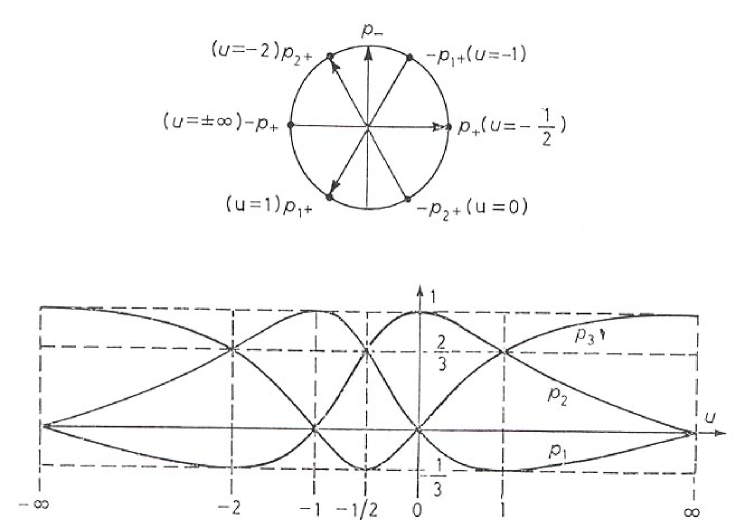
Figure 6: The Lifshitz-Khalatnikov parametrization of the Kasner exponents and of the unit circle in the $p_{+}p_{-}$ plane.

A very useful parametrization of this circle was given by Lifshitz and Khalatnikov [54]

 

$${(p_{1}(u),p_{2}(u),p_{3}(u))}$$

 

The Kasner exponents as functions of the variable $u$ are shown in Figure 6, together with the correspondence with the unit circle in the $p_{+}p_{-}$ plane established by the second equality, which may be inverted to give $u_{\pm}=-{1\over 2}(1\mp[3(1-\hat{p}_{+})/(1+\hat{p}_{+})]^{1\over 2}$, where the upper (lower) sign applies in the upper (lower) half circle. Each of the six sectors into which this circle is divided by the $p_{1+}$, $p_{2+}$, and $p_{3+}$ axes (where the coordinates $\{p_{1+},p_{1-}\}$ and $\{p_{2+},p_{2-}\}$ are obtained from $\{p_{+},p_{-}\}$ by rotations by $2\pi/3$ and $-2\pi/3$ respectively and $\{p_{3+},p_{3-}\}\equiv\{p_{+},p_{-}\}$) represents a different ordering of the same interval of eigenvalues. The intersections of these axes with the circle represent the three permutations of the two inequivalent Taublike case null geodesics whose associated type I spacetime metrics (2.31) are locally rotationally symmetric. If $(a,b,c)$ is a cyclic permutation of (1,2,3) then an interchange of the basis vectors $e_{b}$ and $e_{c}$ leads to reflection across the $\beta^{+}_{a}$ axis in ${\cal M}_{D}$ and hence reflection about the $p_{a+}$ axis in each cotangent space, under which the unit circle is invariant. In terms of the variable $u$ parametrizing this circle, the reflections across the $p_{1+}$, $p_{2+}$ and $p_{3+}$ axes respectively correspond to the discrete transformations $P_{23}(u)=u^{-1}$, $P_{31}(u)=-u(u+1)^{-1}$ and $P_{12}(u)=-(u+1)$ , representing transpositions of the basis vectors $\{e_{a}\}.^{(15)}$ The transformations corresponding to cyclic permutations of these basis vectors leading to rotations of the $\beta^{\pm}$ and $p_{\pm}$ planes by $\pm 2\pi/3$ may be obtained by combining two transpositions. The index permutation $(1,2,3)\to(2,3,1)$ is represented by $P_{231}(u)=P_{23}\circ P_{31}(u)=-u^{-1}(1+u)$, corresponding to a positive rotation by $2\pi/3$ while $(1,2,3)\to(3,1,2)$ is represented by $P_{312}(u)=-(1+u)^{-1}$ , corresponding to a negative rotation by $2\pi/3$ [15].

The diagonal geodesics are characterized by the vanishing of the moment function (2.42) for any offdiagonal matrix B since both K and $\pi$$\pi$$\pi$ are diagonal for these geodesics. Such values for the moment function will be referred to as angular momentum. The constant transformation $f_{\hbox{\bf A }}$ applied to the geodesic (2.46) “transforms away” its constant nonzero angular momentum. For the spacetime metric (2.31) corresponding to (2.46), the new spatial frame $e^{\prime}$ obtained from $e$ by this transformation

$$e_{a}^{\ \prime}=A^{-1b}_{\hskip 13.0pta}e_{b}$$

is an orthogonal frame of eigenvectors of the mixed extrinsic curvature tensor (both g^′ and K^′ are diagonal) . Such a spatial frame is called a Kasner frame and its elements are called Kasner axes [55]. Note, however, that unless $\hbox{\bf A}\in Aut_{e}(g)$, the new structure constant tensor components will differ from the old ones and will in general not belong to ${\cal C}_{D}$. In the analogy with the central force problem, changing the spatial frame by a constant linear transformation corresponds to changing the origin with respect to which the orbital angular momentum is defined.

In the supertime gauge $GL(3,R)$ is the isometry group of the rescaled DeWitt metric so all of its generators are conserved by the (unconstrained) free dynamics. However, invariance of the rescaled curvature potential $NU_{G}$ under the full automorphism group $Aut_{e}(g)$ requires an incompatible time gauge $N\propto g^{-{1\over 2}}$, so $SAut_{e}(g)$ is the largest simultaneous symmetry group of both the kinetic and potential energies.

For a nonvacuum spatially homogeneous spacetime with spatially homogeneous energy-momentum components $T^{\alpha}{}_{\beta}$ in the synchronous gauge, matter variables may usually be chosen so that the matter super-Hamiltonian ${\cal H}_{M}=-2kg^{1\over 2}T^{{}^{\perp}}_{\quad{}_{\perp}}$ acts as a potential function for the matter driving force that appears in the evolution equations. If $d_{{\cal M}}$ is the exterior derivative on ${\cal M}$, then this potential must satisfy

$$T^{\ast}=kg^{1\over 2}T^{ab}dg_{ab}=-d_{{\cal M}}{\cal H}_{M}\ .$$

If this is not possible, one can simply introduce a matter component $Q_{M}$ of the nonpotential force [42]. The matter supermomentum components are ${\cal H}^{M}_{a}=-2kg^{1\over 2}T^{{}^{\perp}}_{\hskip 8.0pta}$ .

The components of the gravitational supermomentum in almost synchronous gauge are defined by [2,42,43]

 

$${{\cal H}^{G}_{a}}$$

 

where the adjoint matrices $\hbox{\bf k}_{a}=C^{b}{}_{ac}\hbox{\bf e}^{c}{}_{b}$ are introduced in appendix A and given explicitly by (A.3). The matrices $\kern-0.24994pt\hbox{$\delta$}\kern-4.44444pt\kern 0.50003pt\hbox{$\delta$}\kern-4.44444pt\kern-0.24994pt\raise 0.43304pt\hbox{$\delta$}_{a}$ generate a subgroup of $SL(3,R)$ which coincides with the linear adjoint group in the class A case and a projective automorphism subgroup in the class B case [2]. These matrices are linearly dependent for Bianchi types I $(\kern-0.24994pt\hbox{$\delta$}\kern-4.44444pt\kern 0.50003pt\hbox{$\delta$}\kern-4.44444pt\kern-0.24994pt\raise 0.43304pt\hbox{$\delta$}_{a}=0)$, type II ($\kern-0.24994pt\hbox{$\delta$}\kern-4.44444pt\kern 0.50003pt\hbox{$\delta$}\kern-4.44444pt\kern-0.24994pt\raise 0.43304pt\hbox{$\delta$}_{1}=0$ when $n^{(1)}\neq 0$, etc.) and type VI_-1/9 $(|n^{(1)}|^{1\over 2}\kern-0.24994pt\hbox{$\delta$}\kern-4.44444pt\kern 0.50003pt\hbox{$\delta$}\kern-4.44444pt\kern-0.24994pt\raise 0.43304pt\hbox{$\delta$}_{1}+|n^{(2)}|^{1\over 2}\kern-0.24994pt\hbox{$\delta$}\kern-4.44444pt\kern 0.50003pt\hbox{$\delta$}\kern-4.44444pt\kern-0.24994pt\raise 0.43304pt\hbox{$\delta$}_{2}=0)$ where the supermomentum constraints are degenerate, imposing additional constraints on the matter supermomentum.

The Einstein evolution equations in almost synchronous gauge are then the equations of motion of the total Lagrangian/Hamiltonian system with the nonpotential force Q and total Lagrangian and Hamiltonian

$$L=L_{G}-N{\cal H}_{M}\ ,\qquad H=H_{G}+N{\cal H}_{M}=N{\cal H}\ ,$$

namely

 

$${-\delta L/\delta g_{ab}}$$

 

These are subject to the constraint equations

$${\cal H}={\cal H}_{G}+{\cal H}_{M}=0,\qquad{\cal H}^{G}_{a}+{\cal H}^{M}_{a}=0\ .$$

For the present paper the source of the gravitational field will be assumed to be a perfect fluid. The appropriate choice of variables and expressions for the fluid super-Hamiltonian, supermomentum and equations of motion are discussed in appendix C.

3 Diagonal Gauge as an Almost Synchronous Gauge Change of Variables

The Einstein equations for a spatially homogeneous spacetime in almost synchronous gauge have been put in the form of a ${\cal C}_{D}$-parametrized constrained classical mechanical system driven by the matter variables which themselves satisfy certain equations of motion. The combined equations of motion are invariant under the action of constant elements of the automorphism matrix group $Aut_{e}(g)$ representing the freedom remaining in the choice of the spatially homogeneous spatial frame in almost synchronous gauge for each fixed point $C^{a}{}_{bc}\in{\cal C}_{D}$. However, only the special automorphism matrix group $SAut_{e}(g)$ acts naturally on the Lagrangian/Hamiltonian system as a symmetry group, corresponding to the additional restriction that the 3-form $\omega^{1}\wedge\,\omega^{2}\wedge\,\omega^{3}$ remain invariant under change of frame, so in this context it is $SAut_{e}(g)$ rather than $Aut_{e}(g)$ which plays an important role [3]. The supermomentum constraint functions are associated with this symmetry, although the direct connection is not so obvious when the nonpotential force is nonzero.

Whenever a dynamical system has a symmetry group, one may simplify the system by choosing new variables adapted to the action of the symmetry group on this system, a very instructive example being the central force problem. Exactly how to adapt the variables depends on the particular way in which the symmetry group acts on the system. For all points of ${\cal C}_{D}$ except the set of measure zero occupied by the type I, II and V orbits, the group $\hat{G}\equiv SAut_{e}(g)$ is 3-dimensional, closely connected to the three linearly independent supermomentum constraint functions, and has an offdiagonal matrix Lie algebra $\hat{g}$ which is such that any point $\hbox{\bf g}\in{\cal M}$ may be diagonalized by one or more elements of this group acting as in (2.16). For the remaining three Bianchi types, $SAut_{e}(g)$ has a larger dimension and for types I and II there are fewer linearly independent supermomentum constraint functions, but there do exist families of 3-dimensional subgroups $\hat{G}$ with offdiagonal Lie algebras which may be used to diagonalize an arbitrary point of ${\cal M}$. Recalling the advantages of diagonal metric component matrices suggests that ${\cal M}_{D}$ should be used to parametrize the orbits of the action of these 3-dimensional groups $\hat{G}$ on ${\cal M}$, leading to the following class of parametrizations $(\beta,\hbox{\bf S})\in diag(3,R)\times\hat{G}\to{\cal M}$

$$\hbox{\bf g}=f^{-1}_{\hbox{\bf S}}(e^{2\kern-0.12251pt\hbox{$\scriptstyle\beta$}\kern-2.77156pt\kern 0.24503pt\hbox{$\scriptstyle\beta$}\kern-2.77156pt\kern-0.12251pt\raise 0.21213pt\hbox{$\scriptstyle\beta$}})=f^{-1}_{\hbox{\bf S}}(\hbox{\bf g}^{\prime})=\hbox{\bf S}^{T}e^{2\kern-0.12251pt\hbox{$\scriptstyle\beta$}\kern-2.77156pt\kern 0.24503pt\hbox{$\scriptstyle\beta$}\kern-2.77156pt\kern-0.12251pt\raise 0.21213pt\hbox{$\scriptstyle\beta$}}\hbox{\bf S}\ ,$$

which decompose the metric matrix variables into “diagonal” and “offdiagonal” variables as described in the introduction. The space $diag(3,R)\sim Diag(3,R)^{+}$ $\sim{\cal M}_{D}$ representing the diagonal variables has already been parametrized in various ways, leaving to be discussed the parametrization of $\hat{G}$ as well as its choice for the type I, II and V cases. For these latter types and the remaining nonsemisimple types, some of the diagonal variables are associated with additional diagonal automorphisms.

The property that the orbit of ${\cal M}_{D}$ under the action of $\hat{G}$ be ${\cal M}$ (in order that any point $\hbox{\bf g}\in{\cal M}$ may be represented in the form (3.1)) requires that the offdiagonal matrix Lie algebra $\hat{g}$ have an ordered basis $\{\kern-0.24994pt\hbox{$\kappa$}\kern-5.76158pt\kern 0.50003pt\hbox{$\kappa$}\kern-5.76158pt\kern-0.24994pt\raise 0.43304pt\hbox{$\kappa$}_{a}\}$ with the property that for each cyclic permutation $(a,b,c)$ of $(1,2,3)$, then $\kern-0.24994pt\hbox{$\kappa$}\kern-5.76158pt\kern 0.50003pt\hbox{$\kappa$}\kern-5.76158pt\kern-0.24994pt\raise 0.43304pt\hbox{$\kappa$}_{a}\in\hbox{span}\{\hbox{\bf e}^{b}{}_{c},\hbox{\bf e}^{c}{}_{b}\}$. Consider the following Lie algebra basis valued function $\{\kern-0.24994pt\hbox{$\kappa$}\kern-5.76158pt\kern 0.50003pt\hbox{$\kappa$}\kern-5.76158pt\kern-0.24994pt\raise 0.43304pt\hbox{$\kappa$}_{a}\}$ on ${\cal C}_{D}$, defined by

 

$${\kern-0.24994pt\hbox{$\kappa$}\kern-5.76158pt\kern 0.50003pt\hbox{$\kappa$}\kern-5.76158pt\kern-0.24994pt\raise 0.43304pt\hbox{$\kappa$}_{a}}$$

 

and satisfying

 

$${[\kern-0.24994pt\hbox{$\kappa$}\kern-5.76158pt\kern 0.50003pt\hbox{$\kappa$}\kern-5.76158pt\kern-0.24994pt\raise 0.43304pt\hbox{$\kappa$}_{a},\kern-0.24994pt\hbox{$\kappa$}\kern-5.76158pt\kern 0.50003pt\hbox{$\kappa$}\kern-5.76158pt\kern-0.24994pt\raise 0.43304pt\hbox{$\kappa$}_{b}]}$$

 

where it is clear from the context when $(a,b,c)$ is to be interpreted as a cyclic permutation of (1,2,3). This is well defined everywhere on ${\cal C}_{D}$ except for the type I, II, IV and V orbits (precisely those points of ${\cal C}_{D}$ where $\hbox{rank}\,\hbox{\bf n}<2$ and the scale matrix $e^{\kern-0.12251pt\hbox{$\scriptstyle\alpha$}\kern-3.13454pt\kern 0.24503pt\hbox{$\scriptstyle\alpha$}\kern-3.13454pt\kern-0.12251pt\raise 0.21213pt\hbox{$\scriptstyle\alpha$}}=\hbox{diag}(e^{\alpha^{1}},e^{\alpha^{2}},e^{\alpha^{3}})$ is singular) where it has direction dependent limits. Consider those points of ${\cal C}_{D}$ for which $n^{(3)}=0$, for example. One then has

 

$${e^{\kern-0.12251pt\hbox{$\scriptstyle\alpha$}\kern-3.13454pt\kern 0.24503pt\hbox{$\scriptstyle\alpha$}\kern-3.13454pt\kern-0.12251pt\raise 0.21213pt\hbox{$\scriptstyle\alpha$}}}$$

 

For type IV only the sign of either $\kern-0.24994pt\hbox{$\kappa$}\kern-5.76158pt\kern 0.50003pt\hbox{$\kappa$}\kern-5.76158pt\kern-0.24994pt\raise 0.43304pt\hbox{$\kappa$}_{1}$ or $\kern-0.24994pt\hbox{$\kappa$}\kern-5.76158pt\kern 0.50003pt\hbox{$\kappa$}\kern-5.76158pt\kern-0.24994pt\raise 0.43304pt\hbox{$\kappa$}_{2}$ does not have a well defined limit for a given orbit, so $\{\kern-0.24994pt\hbox{$\kappa$}\kern-5.76158pt\kern 0.50003pt\hbox{$\kappa$}\kern-5.76158pt\kern-0.24994pt\raise 0.43304pt\hbox{$\kappa$}_{a}\}$ has two values (but a unique $\hat{G}$) for each orbit. In addition to this sign indeterminacy (which does not make $\hat{G}$ multivalued), an $S^{1}$-parametrized family of limits exists for each type II and V orbit component (associated with the indeterminancy of the matrix $\kern-0.24994pt\hbox{$\kappa$}\kern-5.76158pt\kern 0.50003pt\hbox{$\kappa$}\kern-5.76158pt\kern-0.24994pt\raise 0.43304pt\hbox{$\kappa$}_{3}$ for the type V orbit and of the matrix $\kern-0.24994pt\hbox{$\kappa$}\kern-5.76158pt\kern 0.50003pt\hbox{$\kappa$}\kern-5.76158pt\kern-0.24994pt\raise 0.43304pt\hbox{$\kappa$}_{a}$ for the type II orbit component on which $n^{(a)}$ is the only nonvanishing structure constant tensor component), while an $S^{2}$-parametrized family of limits exists for the single type I point containing all well-defined values of this function. Thus $\{\kern-0.24994pt\hbox{$\kappa$}\kern-5.76158pt\kern 0.50003pt\hbox{$\kappa$}\kern-5.76158pt\kern-0.24994pt\raise 0.43304pt\hbox{$\kappa$}_{a}\}$ is a multivalued Lie algebra basis valued function on ${\cal C}_{D}$ whose values at each point determine the offdiagonal diagonalizing automorphism matrix subgroup Lie algebras $\hat{g}$. $\hat{G}$ is then a multivalued matrix Lie group valued function on ${\cal C}_{D}$. (The space of values of this function is diffeomorphic to $S^{2}$ modulo reflection about the origin, namely $P^{2}$.) For the types I, II, IV and V where the multivaluedness occurs, one may pick any value to describe the dynamics.

At the canonical Bianchi type IX point of ${\cal C}_{D}$, $\hat{G}$ has the value $SO(3,R)$ and the parametrization (3.1) reduces to the one introduced by Ryan for all Bianchi types [5]. The latter parametrization arose from considerations completely unrelated to symmetries but by a fortunate coincidence agrees with the correct choice for the most interesting case: Bianchi type IX with canonical structure constant components. Given any frame $e$ with metric component matrix g, there is a natural orthonormal frame related to $e$ by the symmetric square root of g (unique up to ordering when the eigenvalues of g are nondegenerate)

$$\hbox{\bf g}=\hbox{\bf B}^{2}\ ,\qquad B^{a}{}_{b}=B^{b}{}_{a}\ ,\qquad e_{a}^{\prime\prime\prime}=B^{-1b}_{\hskip 13.0pta}e_{a}\ .$$

Since any symmetric matrix can be diagonalized by an orthogonal transformation, ($\hbox{\bf B}=\hbox{\bf O}^{T}\hbox{\bf B}_{D}\hbox{\bf O}\ ,\hbox{\bf O}\in SO(3,R)\ ,\hbox{\bf B}_{D}\in Diag(3,R)^{+}$), using the property $\hbox{\bf O}^{T}=\hbox{\bf O}^{-1}$ one obtains the result $\hbox{\bf g}=\hbox{\bf O}^{T}\hbox{\bf B}_{D}^{\ 2}\hbox{\bf O}$. By setting $\hbox{\bf B}_{D}=e^{\kern-0.12251pt\hbox{$\scriptstyle\beta$}\kern-2.77156pt\kern 0.24503pt\hbox{$\scriptstyle\beta$}\kern-2.77156pt\kern-0.12251pt\raise 0.21213pt\hbox{$\scriptstyle\beta$}}$, one arrives at the Ryan parametrization and its associated orthonormal frame

$$\hbox{\bf g}=\hbox{\bf O}^{T}e^{2\kern-0.12251pt\hbox{$\scriptstyle\beta$}\kern-2.77156pt\kern 0.24503pt\hbox{$\scriptstyle\beta$}\kern-2.77156pt\kern-0.12251pt\raise 0.21213pt\hbox{$\scriptstyle\beta$}}\hbox{\bf O}\ ,\qquad e_{a}^{\prime\prime\prime}=(\hbox{\bf O}^{T}e^{\kern-0.12251pt\hbox{$\scriptstyle\beta$}\kern-2.77156pt\kern 0.24503pt\hbox{$\scriptstyle\beta$}\kern-2.77156pt\kern-0.12251pt\raise 0.21213pt\hbox{$\scriptstyle\beta$}}\hbox{\bf O})^{-1b}_{\hskip 13.0pta}e_{b}=O^{-1c}_{\hskip 13.0pta}(e^{\kern-0.12251pt\hbox{$\scriptstyle\beta$}\kern-2.77156pt\kern 0.24503pt\hbox{$\scriptstyle\beta$}\kern-2.77156pt\kern-0.12251pt\raise 0.21213pt\hbox{$\scriptstyle\beta$}}\hbox{\bf O})^{-1b}_{\hskip 13.0ptc}e_{b}\ .$$

The incompatibility of this parametrization with the symmetry at all points of ${\cal C}$ except for the type I point (where it is unnecessary for perfect fluid spacetimes) and the type IX points where n is proportional to its canonical value made its application to other points of ${\cal C}$ ineffective. (Compare the expressions of the first paper of ref.(23) for the nonpotential force with (3.29).)

If needed one may use the following parametrization of $\hat{G}$

$$\hbox{\bf S}=e^{\theta^{1}\kern-0.12251pt\hbox{$\scriptstyle\kappa$}\kern-2.82318pt\kern 0.24503pt\hbox{$\scriptstyle\kappa$}\kern-2.82318pt\kern-0.12251pt\raise 0.21213pt\hbox{$\scriptstyle\kappa$}_{1}}e^{\theta^{2}\kern-0.12251pt\hbox{$\scriptstyle\kappa$}\kern-2.82318pt\kern 0.24503pt\hbox{$\scriptstyle\kappa$}\kern-2.82318pt\kern-0.12251pt\raise 0.21213pt\hbox{$\scriptstyle\kappa$}_{2}}e^{\theta^{3}\kern-0.12251pt\hbox{$\scriptstyle\kappa$}\kern-2.82318pt\kern 0.24503pt\hbox{$\scriptstyle\kappa$}\kern-2.82318pt\kern-0.12251pt\raise 0.21213pt\hbox{$\scriptstyle\kappa$}_{3}}\ .$$

Suitably restricting the domain of the parameters $\{\theta^{a}\}$ when $\hat{G}$ has compact directions leads to local canonical coordinates of the second kind on $\hat{G}$ (which are always valid in an open neigborhood of the identity if not globally) and hence through (3.1) to local coordinates on each 3-dimensional orbit of $\hat{G}$ on ${\cal M}$. These local coordinates on ${\cal M}$ become singular on $\hat{G}$-orbits of dimension less than three, which represent fixed points of the action of the compact subgroups of $\hat{G}$. The basis $\{\kern-0.24994pt\hbox{$\kappa$}\kern-5.76158pt\kern 0.50003pt\hbox{$\kappa$}\kern-5.76158pt\kern-0.24994pt\raise 0.43304pt\hbox{$\kappa$}_{a}\}$ has the property that when the single parameter $\theta^{a}$ for some fixed value of $a$ is nonzero in (3.7), then (3.1) parametrizes the symmetric case submanifold ${\cal M}_{S(a)}=\{\hbox{\bf g}\in{\cal M}\bigm{|}g_{ab}=g_{ac}=0\}$, where as usual $(a,b,c)$ is a cyclic permutation of (1,2,3). These three submanifolds are associated with discrete spacetime symmetries [43].

Through the parametrization (3.1), the action of $\hat{G}$ on ${\cal M}$

$$\hbox{\bf g}=f^{-1}_{\hbox{\bf S}}(\hbox{\bf g}^{\prime})\to f^{-1}_{\hbox{\bf A}}(\hbox{\bf g})=f^{-1}_{\hbox{\bf SA}^{-1}}(\hbox{\bf g}^{\prime})\ ,\qquad\hbox{\bf A}\in\hat{G}\ ,$$

becomes inverse right translation on $\hat{G}$ itself. Since the DeWitt metric is $SL(3,R)$ invariant and $\hat{G}\subset SL(3,R)$ by virtue of having a tracefree Lie algebra, if a right invariant frame on $\hat{G}$ is employed, the components of the restriction of the DeWitt metric to the orbit (identified with $\hat{G}$) will have components which can at most depend on the diagonal variables.

The relations

 

$${\hbox{\bf S}^{-1}d\hbox{\bf S}}$$

 

define the left and right invariant frames $\{E_{a}\}$ and $\{{\tilde{E}}_{a}\}$ on $\hat{G}$ with respective dual frames $\{W^{a}\}$ and $\{{\tilde{W}}{}^{a}\}$ and structure functions ${\hat{C}}{}^{a}{}_{bc}=W^{a}([E_{a},E_{b}])=-{\tilde{W}}{}^{a}([{\tilde{E}}_{b},{\tilde{E}}_{c}])$ which are naturally associated with the basis $\{\kern-0.24994pt\hbox{$\kappa$}\kern-5.76158pt\kern 0.50003pt\hbox{$\kappa$}\kern-5.76158pt\kern-0.24994pt\raise 0.43304pt\hbox{$\kappa$}_{a}\}$ of its matrix Lie algebra. They satisfy $[E_{a},{\tilde{E}}_{b}]=0$. If $\hbox{\bf S}(\overline{t})$ is a parametrized curve in $\hat{G}$, then

$$\hbox{\bf S}(\overline{t})^{-1}\dot{\hbox{\bf S}}(\overline{t})=\kern-0.24994pt\hbox{$\kappa$}\kern-5.76158pt\kern 0.50003pt\hbox{$\kappa$}\kern-5.76158pt\kern-0.24994pt\raise 0.43304pt\hbox{$\kappa$}_{a}\dot{W}{}^{a}(\overline{t})\quad,\quad\dot{\hbox{\bf S}}(\overline{t})\,\hbox{\bf S}(\overline{t})^{-1}=\kern-0.24994pt\hbox{$\kappa$}\kern-5.76158pt\kern 0.50003pt\hbox{$\kappa$}\kern-5.76158pt\kern-0.24994pt\raise 0.43304pt\hbox{$\kappa$}_{a}{\dot{W}{}}{}^{a}(\overline{t})$$

defines the component functions $\dot{W}{}^{a}(\overline{t})$ and $\dot{W}{}{}^{a}(\overline{t})$ of the curve’s tangent vector with respect to these frames. Let the corresponding functions on the cotangent bundle $T^{\ast}{\hat{G}}$ be denoted by $P_{a}$ and $\tilde{P}_{a}$ respectively. If $\{\theta^{a}\}$ are local coordinates on $\hat{G}$, then one has the following coordinate expressions for the right invariant frame quantities

 

$${{\tilde{E}}_{a}}$$

 

where $\{\theta^{a},{\dot{\theta}}{}^{a}\}$ and $\{\theta,p_{a}\}$ are the natural lifted coordinates on the tangent and cotangent bundles. Dropping the tildes leads to the corresponding left invariant frame quantities which are related by the linear adjoint transformation on $\hat{G}$

 

$${\hbox{\bf S}\kern-0.24994pt\hbox{$\kappa$}\kern-5.76158pt\kern 0.50003pt\hbox{$\kappa$}\kern-5.76158pt\kern-0.24994pt\raise 0.43304pt\hbox{$\kappa$}_{a}\hbox{\bf S}^{-1}}$$

 

One may also use the local canonical coordinates $(\theta^{a},p_{a})$ to evaluate the following Poisson brackets

 

$${{}\{{\tilde{P}}_{a},{\tilde{P}}_{b}\}={\hat{C}}{}^{c}{}_{ab}{\tilde{P}}_{c}\qquad\{\hbox{\bf S},{\tilde{P}}_{a}\}=\kern-0.24994pt\hbox{$\kappa$}\kern-5.76158pt\kern 0.50003pt\hbox{$\kappa$}\kern-5.76158pt\kern-0.24994pt\raise 0.43304pt\hbox{$\kappa$}_{a}\hbox{\bf S}}$$

 

Since the basis $\{\kern-0.24994pt\hbox{$\kappa$}\kern-5.76158pt\kern 0.50003pt\hbox{$\kappa$}\kern-5.76158pt\kern-0.24994pt\raise 0.43304pt\hbox{$\kappa$}_{a}\}$ is closely related to the standard basis of one of the standard diagonal form adjoint matrix Lie algebras with rank n $>1$, explicit expressions may easily be obtained from the formulas of appendix A for S, $\hat{\hbox{\bf R}}$ and the component matrices of the invariant fields in terms of the parametrization (3.7). The case $n^{(3)}=0$ is given as an example in that appendix.

The parametrization (3.1) has the following meaning. Given the spacetime metric (2.24) is some almost synchronous gauge, i.e. given the parametrized curve $\hbox{\bf g}(\overline{t})$ in ${\cal M}$ and the lapse function $N(\overline{t})$, then $\hbox{\bf A}(\overline{t})=\hbox{\bf S}(\overline{t})$ is the matrix in (2.27) which affects the change to diagonal gauge, where the new metric matrix $\overline{\hbox{\bf g}}(\overline{t})=\hbox{\bf g}^{\prime}(\overline{t})$ is diagonal and the new spatial frame

$$e_{a}^{\ \prime}=S^{-1b}_{\hskip 13.0pta}(\overline{t})e_{b}$$

is orthogonal, with the associated shift vector field satisfying

$$\hbox{ad}_{e^{\prime}}(\vec{N}(\overline{t}))=\kern-0.24994pt\hbox{$\kappa$}\kern-5.76158pt\kern 0.50003pt\hbox{$\kappa$}\kern-5.76158pt\kern-0.24994pt\raise 0.43304pt\hbox{$\kappa$}_{a}{\dot{W}{}}{}^{a}\ ,$$

according to (2.33). The matrix $e^{\kern-0.12251pt\hbox{$\scriptstyle\beta$}\kern-2.77156pt\kern 0.24503pt\hbox{$\scriptstyle\beta$}\kern-2.77156pt\kern-0.12251pt\raise 0.21213pt\hbox{$\scriptstyle\beta$}}\in Diag(3,R)^{+}$ then normalizes this orthogonal spatial frame, leading to the natural symmetry adapted orthonormal spatial frame

$$e_{a}^{\prime\prime}=(e^{\kern-0.12251pt\hbox{$\scriptstyle\beta$}\kern-2.77156pt\kern 0.24503pt\hbox{$\scriptstyle\beta$}\kern-2.77156pt\kern-0.12251pt\raise 0.21213pt\hbox{$\scriptstyle\beta$}})^{-1b}_{\hskip 13.0pta}e_{b}^{\prime}=(e^{\kern-0.12251pt\hbox{$\scriptstyle\beta$}\kern-2.77156pt\kern 0.24503pt\hbox{$\scriptstyle\beta$}\kern-2.77156pt\kern-0.12251pt\raise 0.21213pt\hbox{$\scriptstyle\beta$}}\hbox{\bf S})^{-1b}_{\hskip 13.0pta}e_{b}$$

which may be used to introduce spinor fields on the spacetime in “time gauge” [42,56,57] or to introduce a natural Newman-Penrose null tetrad or to put the Einstein equations in a simple form without a Lagrangian/Hamiltonian formulation [58]. The offdiagonal velocities ${\dot{W}{}}{}^{a}$ are linearly related to the angular velocity of this natural spatial triad relative to one which is parallelly propagated along the normal congruence [42]. Note that in the canonical type IX case, this orthonormal spatial frame differs from the frame (3.6) which is associated with the Ryan parametrization by an additional rotation, and like that frame, is unique modulo ordering of the frame vectors and barring degeneracies for each value of $\hat{G}$.

Let a prime indicate components with respect to the diagonal gauge spatial frame (3.14). As noted in the previous section, spatial curvatures have simpler expressions in diagonal gauge; in particular the scalar curvature potential function $U_{G}$ is independent of the offdiagonal variables and is simply given by the formula (2.27). The extrinsic curvature (2.36) and the kinetic energy have the following expressions when evaluated with respect to the primed frame

 

$${\hbox{\bf K}^{\prime}}$$

 

indicating that the DeWitt metric itself is

$${\textstyle{1\over 4}}{\cal G}=e^{3\beta^{0}}(6\eta_{AB}d\beta^{A}\otimes d\beta^{B}+\overline{{\cal G}}_{ab}{\tilde{W}}{}^{a}\otimes{\tilde{W}}{}^{b})\ .$$

The components of the rescaled DeWitt metric $\overline{{\cal G}}\equiv{1\over 4}g^{-{1\over 2}}{\cal G}$ along the orbit directions are functions on the $\beta^{+}\beta^{-}$ plane and are diagonal due to the choice of basis (3.2) of $\hat{g}$

$$\overline{{\cal G}}_{aa}={\textstyle{1\over 2}}e^{-2\alpha^{a}}(n^{(b)}e^{\beta^{bc}}-n^{(c)}e^{-\beta^{bc}})^{2}\equiv(\overline{{\cal G}}{}^{-1\ aa})^{-1}\ .$$

When $(e^{-\alpha^{a}}n^{(b)},e^{-\alpha^{a}}n^{(c)})$ equals respectively $(\sqrt{2},0)$, $(1,-1)$ and $(1,1)$, as occurs at canonical points of ${\cal C}_{D}$, this expression has the values $e^{2\beta^{bc}}$, $2\hbox{cosh}^{2}\beta^{bc}$ and $2\hbox{sinh}^{2}\beta^{bc}$. When $\kern-0.24994pt\hbox{$\kappa$}\kern-5.76158pt\kern 0.50003pt\hbox{$\kappa$}\kern-5.76158pt\kern-0.24994pt\raise 0.43304pt\hbox{$\kappa$}_{a}$ is a compact generator, which means that $e^{-\alpha^{a}}n^{(b)}$ and $e^{-\alpha^{a}}n^{(c)}$ are nonzero and of the same sign, then $\overline{{\cal G}}_{aa}$ vanishes for

$$\beta^{-}_{a}=\beta^{-}_{a0}\equiv-(4\sqrt{3})^{-1}\ln|e^{-\alpha^{a}}n^{(b)}/e^{-\alpha^{a}}n^{(c)}|$$

which for canonical points of ${\cal C}_{D}$ represents the 2-dimensional orbit of the Taub submanifold ${\cal M}_{T(a)}$. Such points of ${\cal M}$ represent singularities of the parametrization (3.1). This same condition on $\beta^{-}_{a}$ picks out the submanifold of ${\cal M}_{D}$ for which $d\overline{{\cal G}}_{aa}=0=d\overline{{\cal G}}{}^{-1aa}$ when $e^{-\alpha^{a}}n^{(b)}$ and $e^{-\alpha^{a}}n^{(c)}$ are both nonzero.

The velocity-momentum relations following from the above kinetic energy are

 

$${p_{A}}$$

 

Re-expressing the gravitational momentum (2.38) in terms of these momenta using (3.15) leads to

$$\kern-0.24994pt\hbox{$\pi$}\kern-5.70027pt\kern 0.50003pt\hbox{$\pi$}\kern-5.70027pt\kern-0.24994pt\raise 0.43304pt\hbox{$\pi$}^{\prime}=\hbox{\bf S}\kern-0.24994pt\hbox{$\pi$}\kern-5.70027pt\kern 0.50003pt\hbox{$\pi$}\kern-5.70027pt\kern-0.24994pt\raise 0.43304pt\hbox{$\pi$}\hbox{\bf S}^{-1}={\textstyle{1\over 12}}(\eta^{AB}p_{A}\hbox{\bf e}_{B}+3p_{0}\hbox{\bf e}_{0})+{\textstyle{1\over 2}}\overline{{\cal G}}{}^{-1ab}{\tilde{P}}_{a}\kern-0.24994pt\hbox{$\kappa$}\kern-5.76158pt\kern 0.50003pt\hbox{$\kappa$}\kern-5.76158pt\kern-0.24994pt\raise 0.43304pt\hbox{$\kappa$}_{b}^{\#\ \prime}\ .$$

Defining

$$P^{\prime}(\hbox{\bf A})=-2\hbox{Tr}\,\kern-0.24994pt\hbox{$\pi$}\kern-5.70027pt\kern 0.50003pt\hbox{$\pi$}\kern-5.70027pt\kern-0.24994pt\raise 0.43304pt\hbox{$\pi$}^{\prime}\hbox{\bf A}\ ,\qquad\hbox{\bf A}\in gl(3,R)\ ,$$

one finds

$$p_{A}=-P^{\prime}(\hbox{\bf e}_{A})\ ,\qquad{\tilde{P}}_{a}=-P^{\prime}(\kern-0.24994pt\hbox{$\kappa$}\kern-5.76158pt\kern 0.50003pt\hbox{$\kappa$}\kern-5.76158pt\kern-0.24994pt\raise 0.43304pt\hbox{$\kappa$}_{a})\ ,$$

the minus sign arising from the inverse action used in the parametrization (3.1) to conform with other conventions. Note that the canonical generators of the action (3.8) of $\hat{G}$ on ${\cal M}$ are instead (using (2.43), (3.12), (3.22) and (3.23))

$$P(\kern-0.24994pt\hbox{$\kappa$}\kern-5.76158pt\kern 0.50003pt\hbox{$\kappa$}\kern-5.76158pt\kern-0.24994pt\raise 0.43304pt\hbox{$\kappa$}_{a})=P^{\prime}(\hbox{\bf S}\kern-0.24994pt\hbox{$\kappa$}\kern-5.76158pt\kern 0.50003pt\hbox{$\kappa$}\kern-5.76158pt\kern-0.24994pt\raise 0.43304pt\hbox{$\kappa$}_{a}\hbox{\bf S}^{-1})=P^{\prime}(\kern-0.24994pt\hbox{$\kappa$}\kern-5.76158pt\kern 0.50003pt\hbox{$\kappa$}\kern-5.76158pt\kern-0.24994pt\raise 0.43304pt\hbox{$\kappa$}_{b}){\hat{R}}{}^{b}{}_{a}=-P_{a}\ ,$$

namely the left invariant frame momenta. Finally, re-expressing the kinetic energy as a function on momentum phase space leads to

$$N{\cal T}={\textstyle{1\over 2}}N(12e^{3\beta^{0}})^{-1}(\eta^{AB}p_{A}p_{B}+6\overline{{\cal G}}{}^{-1ab}{\tilde{P}}_{a}{\tilde{P}}_{b})$$

The action (3.8) of $\hat{G}$ is a symmetry of the free Hamiltonian dynamics generated by the kinetic energy function alone and hence the canonical generators $P_{a}$ are conserved; this is clear from (3.26) since $P_{a}$ commute with $N{\cal T}$ provided that $N$ is $\hat{G}$-invariant. The momenta $\tilde{P}_{a}$ are related to the conserved momenta by the time dependent adjoint transformation.

To summarize, $\{\partial/\partial\beta^{A},{\tilde{E}}_{a}\}$ represents through the parametrization (3.1) an orthogonal frame on ${\cal M}$ adapted to the three-plus-three decomposition of ${\cal M}$ into orbits of the action of $\hat{G}$ (offdiagonal or “angular” variables) and their orthogonal submanifolds (diagonal or “radial” variables). In Misner’s supertime time gauge $N=12e^{3\beta^{0}}$, the diagonal part of the kinetic energy is simply the standard kinetic energy of the flat Lorentz geometry of the metric space $(diag(3,R),\langle\langle,\rangle\rangle_{{}_{DW}})$ expressed in inertial coordinates $\{\beta^{A}\}$, while the offdiagonal part of the kinetic energy is just the one associated with the right invariant metric $I={1\over 6}\overline{{\cal G}}_{ab}{\tilde{W}}{}^{a}\otimes{\tilde{W}}{}^{b}$ on $\hat{G}$, the two pieces coupled together by the $\beta^{\pm}$ dependence of the components $I_{ab}={1\over 6}\overline{{\cal G}}_{ab}$.

The offdiagonal dynamics is thus governed by the natural generalization of the rigid body dynamics at the canonical type IX point of ${\cal C}_{D}$ where $\hat{G}=SO(3,R)$ to the (multivalued) matrix group $\hat{G}$ at each point of ${\cal C}_{D}$. This is discussed at length for a general Lie group by Abraham and Marsden in a more abstract notation [46]. The spatial frames $e$ and $e^{\prime}$ are respectively identified with the space-fixed and body-fixed axes, related by the passive transformation S which corresponds to Goldstein’s matrix A of his equation (4.46) [45], the value assumed by S for the canonical type IX point of ${\cal C}_{D}$ when expressed in his Euler angle parametrization of $SO(3,R)$. Here $(-\dot{W}{}^{a},{-\dot{W}{}}{}^{a})$ and $(-P_{a},-{\tilde{P}}_{a})$ play the roles of the space-fixed and body-fixed components of the angular velocity and spin angular momentum of the rigid body, and in a general time gauge, $I_{(a)}=2N^{-1}e^{3\beta^{0}}\overline{{\cal G}}_{aa}$ play the role of the principal moments of inertia, namely the eigenvalues of the moment of inertia tensor $I$. Notice that it is the space-fixed components of the angular momentum which are conserved by the free dynamics, exactly as in the force free rigid body case; however, it is the principal (body-fixed) axes of the moment of inertia tensor will allow one to solve the equations of motion for that case. It is this fact which motivates diagonal gauge in the present problem.

The identification of S with the passive coordinate transformation from space-fixed to body-fixed coordinates leads to the minus sign which arises here and in (3.24). The parametrization (3.1) with $f$ rather than $f^{-1}$ would lead to the identification of S with the active transformation from the space-fixed basis vectors to the body-fixed basis vectors (Goldstein’s matrix A^-1), eliminating the minus sign and interchanging left and right in the above discussion. For the type IX case, this rigid body analogy is simply the restriction to symmetry compatible diffeomorphisms and subsequent translation into frame language of the Fischer-Marsden discussion for general spatially compact spacetimes. The finite dimensional situation here allows the analogy to be carried much further.

On the other hand, the left invariant frame momenta $P_{a}$ generate the canonical action of $\hat{G}$ on the momentum phase space and thus act like orbital angular momenta in the central force problem, leading to the analogy in which the radial and angular variables correspond to the diagonal and offdiagonal variables of the present system. The fact that this action of $\hat{G}$ arises from the action of spatial diffeomorphisms on the spacetime metric (2.31) makes the decomposition into diagonal and offdiagonal variables relevant to the Einstein equations.

A key feature of this decomposition is the resulting trivialization of the supermomentum constraints (which are in general intimately connected with the spatial diffeomorphism group) and of the nonpotential force. These involve the matrices $\{\kern-0.24994pt\hbox{$\delta$}\kern-4.44444pt\kern 0.50003pt\hbox{$\delta$}\kern-4.44444pt\kern-0.24994pt\raise 0.43304pt\hbox{$\delta$}_{a}\}$ introduced in (2.51) and given explicitly by

$$\kern-0.24994pt\hbox{$\delta$}\kern-4.44444pt\kern 0.50003pt\hbox{$\delta$}\kern-4.44444pt\kern-0.24994pt\raise 0.43304pt\hbox{$\delta$}_{1}=-n^{(2)}\hbox{\bf e}^{3}{}_{2}+n^{(3)}\hbox{\bf e}^{2}{}_{3}-3a\hbox{\bf e}^{3}{}_{1}\hfil$$

which leads to the definition of a matrix $\rho$$\rho$$\rho$ by

$$\kern-0.24994pt\hbox{$\delta$}\kern-4.44444pt\kern 0.50003pt\hbox{$\delta$}\kern-4.44444pt\kern-0.24994pt\raise 0.43304pt\hbox{$\delta$}_{a}=\kern-0.24994pt\hbox{$\kappa$}\kern-5.76158pt\kern 0.50003pt\hbox{$\kappa$}\kern-5.76158pt\kern-0.24994pt\raise 0.43304pt\hbox{$\kappa$}_{b}\rho^{b}{}_{a}+a_{a}\hbox{\bf e}_{+}\ .$$

The nonpotential force is then evaluated as follows

 

$${Q}$$

 

Note that the $\beta^{+}$ component of the nonpotential force exactly cancels the $\beta^{+}$ component of the Einstein force arising from the exterior derivative of the $a^{2}$ term in the expression (2.27) for $U_{G}$

$$Q_{+}-\partial/\partial\beta^{+}(6a^{2}e^{\beta^{0}+4\beta^{+}})=0\ ,$$

i.e., only the first term $e^{\beta^{0}}V^{\ast}$ is relevant to the equations of motion for the $\beta^{\pm}$ variables. (Subtraction of this second term from $U_{G}$ in the Lagrangian or Hamiltonian would require the introduction of a $\beta^{0}$ component of $Q$; if $\beta^{0}$ is determined by integrating the super-Hamiltonian constraint rather than by equations of motion, this is irrelevant, leaving only the component $Q_{3}$ as relevant to the remaining equations of motion and which vanishes for Bianchi type V.)

The primed gravitational supermomentum components are given by

$${\cal H}_{a}^{G\ \prime}=P^{\prime}(\kern-0.24994pt\hbox{$\delta$}\kern-4.44444pt\kern 0.50003pt\hbox{$\delta$}\kern-4.44444pt\kern-0.24994pt\raise 0.43304pt\hbox{$\delta$}_{a})=-{\tilde{P}}_{b}\rho^{b}{}_{a}-a_{a}p_{+}\ .$$

As already noted, these are linearly dependent for Bianchi types I, II and VI_-1/9. This is reflected by the vanishing of $\det\kern-0.24994pt\hbox{$\rho$}\kern-5.17015pt\kern 0.50003pt\hbox{$\rho$}\kern-5.17015pt\kern-0.24994pt\raise 0.43304pt\hbox{$\rho$}=[e^{\alpha^{1}}e^{\alpha^{2}}+9a^{2}\hbox{sgn}(n^{(1)}n^{(2)})]e^{\alpha^{3}}$ which has the class A value $e^{\alpha^{1}+\alpha^{2}+\alpha^{3}}$ and the class B value $|n^{(1)}n^{(2)}|(1+9h)e^{\alpha^{3}}$. This also vanishes for Bianchi type V where $e^{\alpha^{3}}=0$.

For the remaining types one may solve the supermomentum constraints for the offdiagonal momenta or velocities

 

$${\tilde{P}_{a}}$$

 

and thus determine the diagonal gauge shift vector field (3.15) modulo time dependent elements of $\tilde{g}$ (spatial Killing vector fields). This is essentially just an application of the thin sandwhich formulation of the initial value problem [59,60]; initial values of $(\hbox{\bf g}^{\prime},\dot{\hbox{\bf g}}^{\prime},{\cal H}_{a}^{M\ \prime})$ are specified arbitrarily and the supermomentum constraints are used to determine the diagonal gauge shift variables. For Bianchi type V the diagonal/offdiagonal decomposition is not compatible with the thin sandwhich interpretation since the diagonal momentum $p_{+}$ rather than the offdiagonal momentum $\tilde{P}_{3}$ is constrained, while for types I, II and VI_-1/9 certain shift components (i.e. offdiagonal momenta) remain freely specifiable initial data due to the degeneracy of the constraints. The important distinction between the present case and the thin sandwhich interpretation is that here the shift variables have been made velocities associated with dynamical variables and the supermomentum constraints allow one to determine the shift variables directly at each moment of time rather than by integrating their (first order) equations of motion.

The idea of incorporating the shift variables into the dynamics as the velocities associated with gauge variables was developed by Fischer and Marsden [46]. Their construction when adapted to the spatially homogeneous case extends the configuration space ${\cal M}$ to ${\cal M}\times R\times Aut_{e}(g)$ with natural variables $(\hbox{\bf g},t,\hbox{\bf A})$ and velocities $(\dot{\hbox{\bf g}},\dot{t}=N,\dot{\hbox{\bf A}}\hbox{\bf A}^{-1}=\hbox{ad}_{\overline{e}}(\vec{N}))$ whose interpretation is the same as in (2.31)-(2.35). Imposition of the $\hat{G}$-diagonalization gauge condition $(\hbox{\bf g},\hbox{ad}_{\overline{e}}(\vec{N}))\in{\cal M}_{D}\times\hat{g}$ on this extended system then leads to the results of the present approach.

Thus the diagonal/offdiagonal decomposition of the almost synchronous gauge gravitational variables leads automatically to the diagonal gauge equations of motion, while the diagonal gauge supermomentum constraints then determine the diagonal gauge shift variables which appear in these equations of motion, except in the degenerate cases (Bianchi types I, II, V and VI_-1/9) where first order equations of motion for the undetermined shift variables must be used to evolve them. These first order equations may be obtained directly in Hamiltonian form by using the Poisson bracket relations (3.13). (For the vacuum dynamics these are just generalized Euler equations with time dependent principal moments of inertia, driven by the additional nonpotential force component $Q_{3}$ in the class B case.) To complete this scheme one needs to introduce the diagonal gauge matter variables by a time dependent change of variables involving the transformation matrix S, leading to the appearance of shift terms in the new matter equations of motion through (3.15). These terms are analogous to the centrifugal force which appears in the rotating body-fixed frame of the rigid body problem.

The combined Einstein and matter equations then involve only diagonal gauge variables and the diagonal gauge shift variables which are in general determined by the supermomentum constraints (or by first order equations of motion if not). The spacetime metric may then be represented directly in diagonal gauge form, without integrating the equations which determine S, the transformation back to almost synchronous gauge. The offdiagonal part of the kinetic energy then acts like a time dependent effective potential for the diagonal gauge gravitational variables, which from the central force analogy has been called the centrifugal potential by Ryan [20,21]. The matter super-Hamiltonian acts as another time dependent potential for these variables.

For a perfect fluid source as discussed in appendix C, the appropriate variables are $(n,l,v_{a})$; the diagonal gauge variables are defined by (C.3) with $\hbox{\bf A}\,=\,\hbox{\bf S}$, namely

$$(n^{\prime},l^{\prime},v_{a}^{\prime})=(n,l,v_{b}S^{-1b}_{\hskip 13.0pta})\ .$$

The primed components of the matter supermomentum and the matter super-Hamiltonian then have the expressions

 

$${{\cal H}^{M\ \prime}_{a}}$$

 

In the Bianchi type I dust (zero pressure) case, Ryan has called the first term in the matter super-Hamiltonian the rotation potential since it directly influences the gravitational variables only when the fluid is tilted ($v_{a}\neq 0$) [61] and tilt is equivalent to rotation of the fluid in this case. However, for the remaining types tilt and nonzero rotation ($C^{ab}v_{b}\neq 0$) are no longer synonymous [43], so tilt potential is a better name. Let ${\cal H}^{tilt}_{M}$ designate this potential. The second term or pressure potential only affects the equations of motion for $\beta^{0}$.

To evaluate the equations of motion for the offdiagonal momenta, one needs the following Poisson brackets which are a consequence of (3.13) and (3.33)

$$\{{\tilde{P}}_{a},v^{\prime}_{b}\}=v_{c}^{\prime}\kappa_{a\hskip 4.0ptb}^{\hskip 4.0ptc}\qquad\{P_{a},v^{\prime}_{b}\}=v^{\prime}_{c}\kappa^{\hskip 4.0ptc}_{d\hskip 4.0ptb}{\hat{R}}{}^{d}{}_{a}\ .$$

One then finds the result

 

$${({\tilde{P}}_{a}){\dot{\ }}}$$

 

For the free dynamics and class A vacuum dynamics ($Q_{a}=0=F_{a}$), these equations generalize the Euler equations for the body-fixed components of the angular momentum of a rigid body, and like those equations conserve the space-fixed components of the angular momentum. For the class B vacuum dynamics the component $Q_{3}$ appears as a driving term and the conserved quantities are instead the unprimed supermomentum components

 

$${{\cal H}^{G}_{a}}$$

 

The momenta $P_{1}$ and $P_{2}$ are conserved by the vacuum dynamics, being constant linear combinations of ${\cal H}^{G}_{1}$ and ${\cal H}^{G}_{2}$, but $P_{3}$ is not unless $Q_{3}=0$. Because of the supermomentum constraints (3.32), the equations of motion for the offdiagonal momenta $\tilde{P}_{a}$ are very closely related to the primed fluid equations of motion which may be obtained by transforming (C.5)

$$\dot{l}=Nl(v^{\bot})^{-1}\,2a^{\prime c}v^{\prime}_{c}\qquad(v^{\prime}_{a})\dot{\ }\ =Nv^{\prime}_{b}[(v^{\bot})^{-1}C^{b}{}_{ca}v^{\prime c}-\kappa^{\hskip 4.0ptb}_{c\hskip 4.0pta}\dot{W}{}{}^{c}]$$

The lapse $N$ is still arbitrary and the super-Hamiltonian constraint remains to be dealt with. Several options are available. Introduce the function $I_{\tilde{h}}$ depending on an arbitrary real parameter $\tilde{h}$ by

$$I_{\tilde{h}}=-(\hbox{sgn}\,p_{0})[24e^{3\beta^{0}}({\cal H}+\tilde{h})+p_{0}^{\ 2}]^{1\over 2}\ ,$$

enabling the super-Hamiltonian constraint to be expressed in the compact form

$${\cal H}={\textstyle{1\over 24}}e^{-3\beta^{0}}(-p^{\ 2}_{0}+I_{0}^{\ 2})=0\ ,$$

which suggests that it be used to solve for $p_{0}$, the result being $p_{0}=-I_{0}$. ($p_{0}$ is negative for expansion or increasing $\beta^{0}$ with increasing proper time and is positive for contraction.)

Suppose one initially assumes unit lapse function, so that the time of the classical mechanical system coincides with the proper time $t$ on the spacetime. The super-Hamiltonian constraint may then be used to eliminate another degree of freedom from the system by a standard technique of classical mechanics [1] which replaces the time $t$ as the integration variable by some function $\overline{t}$ of $\beta$$\beta$$\beta$ (accomplished by changing the independent variable in the action). This is called an “intrinsic time reduction” of the system [62]. The usual and obvious choice is $\overline{t}=\beta^{0}=-\Omega$ or negative $\Omega$-time. ($\Omega$-time is useful for approaching the initial singularity.) This is clearly equivalent to specifying a new lapse function $N$. The reduction technique leads to the reduced Hamiltonian $I_{0}$ and equations of motion

$${\dot{\beta}}{}^{\pm}=\{\beta^{\pm},I_{0}\}\ ,\qquad{\dot{p}}_{\pm}=\{p_{\pm},I_{0}\}+\delta^{+}{}_{\pm}NQ_{+}\ ,$$

where the new lapse function $N$ is determined by the first order equation for the original time $t$

$$N=\dot{t}=\partial I_{\tilde{h}}/\partial{\tilde{h}}\bigm{|}_{\tilde{h}=0}=12e^{3\beta^{0}}I_{0}^{\ -1}$$

and the dot refers to the new time derivative.

This same result can also be obtained by simply setting $N=-12e^{3\beta^{0}}p_{0}^{\ -1}$ in the original Hamiltonian $H=N{\cal H}$

 

$${H}$$

 

the result ${\dot{\beta}}{}^{0}=1$ following from the imposition of the constraint $p_{0}=-I_{0}$. For any variable $y$ other than $p_{0}$, one has $\partial H/\partial y=(-p_{0}^{\ -1}I_{0})\partial I_{0}/\partial y$, showing that $I_{0}$ acts as the Hamiltonian for all variables but $\beta^{0}$ when the constraint $p_{0}=-I_{0}$ is imposed. Misner’s supertime time gauge $N=12e^{3\beta^{0}}$ differs differs only by eliminating the factor $-p_{0}$ in the $\beta^{0}$-time lapse function, leading to a Hamiltonian of familiar form rather than a square root Hamiltonian as above

$$H=-{\textstyle{1\over 2}}p_{0}^{\ 2}+{\textstyle{1\over 2}}I_{0}^{\ 2}\ .$$

In this time gauge, ${1\over 2}I_{0}^{\ 2}$ acts as the Hamiltonian for the variables other than $(\beta^{0},p_{0})$ and the super-Hamiltonian constraint ${\dot{\beta}}{}^{0}=-p_{0}=I_{0}$ may be used to evolve $\beta^{0}$. Note that

 

$${{\textstyle{1\over 2}}I_{0}^{\ 2}}$$

 

The term $H_{eff}$ acts as an effective Hamiltonian for the variables other than $(\beta^{0},p_{0})$; the corresponding Hamiltonian equations of motion for the $\beta^{\pm}$ degrees of freedom contain no nonpotential force.

Whatever the time gauge, one may introduce an effective Hamiltonian for the $\beta^{\pm}$ degrees of freedom by subtracting out the $p_{0}^{\ 2}$ term, the pressure potential and the $a^{2}$ term in the scalar curvature potential

 

$${H_{eff}}$$

 

As discussed above, the use of $H_{eff}$ rather than $H$ eliminates the need to consider the nonpotential force component $Q_{+}$, so $H_{eff}$ alone generates the correct equations of motion for the $\beta^{\pm}$ degrees of freedom. The component $Q_{3}$ is still relevant to the equations of motion for the offdiagonal variables, when needed, for which either $H$ or $H_{eff}$ may be used. A nonvanishing value of $Q_{3}$ is connected with the single nonvanishing offdiagonal component of the spatial Ricci tensor in diagonal gauge (see (2.25)).

One advantage of the supertime time gauge is that the kinetic energy for the diagonal variables corresponds to a relativistic particle in the flat 3-dimensional spacetime ($diag(3,R)$, $\eta_{AB}d\beta^{A}\otimes d\beta^{B}$). Neglecting the remaining terms in the Hamiltonian (the free system with zero orbital angular momentum), one obtains affinely parametrized geodesics for the system trajectories and the Hamiltonian constraint just requires that the particle velocity be null. Except for small anisotropy in the type IX case, the remaining terms are all positive (although the pressure potential is negative, the total fluid Hamiltonian is positive) and their effect is therefore to make the particle velocity timelike. It is future pointing in the case of expansion ($\beta^{0}$ increasing) and past pointing in the case of contraction ($\beta^{0}$ decreasing), reversing direction only in the type IX case where recollapse occurs.

The $\beta^{0}$-time gauge, on the other hand, uses the natural time variable $\beta^{0}$ of the 3-dimensional flat spacetime to parametrize the system trajectories; for the geodesics it is also an affine parameter. This has the advantage of making the reduced Hamiltonian for the $\beta^{\pm}$ degrees of freedom explicitly rather than implicitly time dependent.

The curvature potential $V^{\ast}$ has been described and diagrammed in the previous section and enters the Hamiltonian in the supertime time gauge as the time dependent potential $U_{g}=12e^{4\beta^{0}}V^{\ast}$, which apart from constants has been called the gravitational potential by Ryan [20,21]. The centrifugal potential

$$U_{c}=3\overline{{\cal G}}{}^{-1ab}{\tilde{P}}_{a}{\tilde{P}}_{b}=3\sum_{n=1}^{3}\overline{{\cal G}}{}^{-1ab}{\tilde{P}}^{\ 2}_{a}\equiv\sum_{n=1}^{3}U_{c}^{(a)}$$

is the sum of three terms whose $\beta^{\pm}$ dependence is given by (3.19) and is repeated in a more suggestive form here.

$$\hfil(i)$$

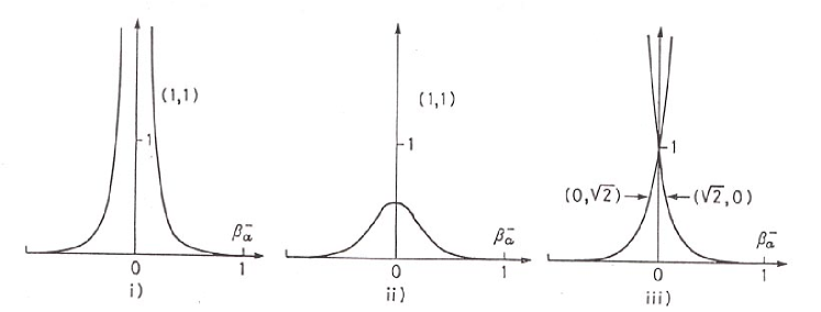
Figure 7: Plots of $\overline{{\cal G}}{}^{-1aa}$ for canonical points of ${\cal C}_{D}$, at which the pair $e^{-\alpha^{a}}(n^{(b)},n^{(c)})$ assumes the values shown.

These are illustrated for the canonical points of ${\cal C}_{D}$ in Figure 7. The potentials for noncanonical points arise from these by a combined rescaling and translation, infinite translations corresponding to Lie algebra contractions. All of these potentials are exponentially cut off in one or both directions. Case $(i)$ corresponds to a compact generator $\kern-0.24994pt\hbox{$\kappa$}\kern-5.76158pt\kern 0.50003pt\hbox{$\kappa$}\kern-5.76158pt\kern-0.24994pt\raise 0.43304pt\hbox{$\kappa$}_{a}$ in which the potential behaves like $(\beta^{-}_{a})^{-2}$ at the origin, exactly as in the central force problem where the centrifugal potential has the dependence $r^{-2}$ on the radial coordinate $r$. Thus the singularities of the parametrization (3.1) are shielded by angular momentum barriers exactly like the spherical coordinate singularity at the origin in the central force problem. Case $(ii)$ also acts like an angular momentum barrier but can be overcome if the energy of the system is sufficiently large. In case $(iii)$ the barriers have been translated out to infinity. In the supertime time gauge, all of the time dependence of the centrifugal potentials arises from the angular momentum factors. Increasing ${\tilde{P}}{}_{a}^{\ 2}$ increases $U_{c}^{(a)}$ and causes a given value of the potential to move in the direction of decreasing values. The barrier $(i)$ may be crossed provided that the relevant angular momentum component vanishes at the moment of crossing.

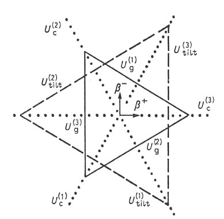
Figure 8: The key to Figure 9. Together with Figure 2, this shows the $\beta^{\pm}_{a}$ coordinate associated with each potential represented in Figure 9 by wall contours. In general the wall contours associated with tilt and type $(iii)$ centrifugal potentials will be translated from their symmetrical positions. The dotted lines for the type $(i)$ and $(ii)$ centrifugal potential contours in Figure 9 have double arrows since they actually represent a pair of contours symmetrically located with respect to the point at which the potential becomes infinite or assumes its maximum value.

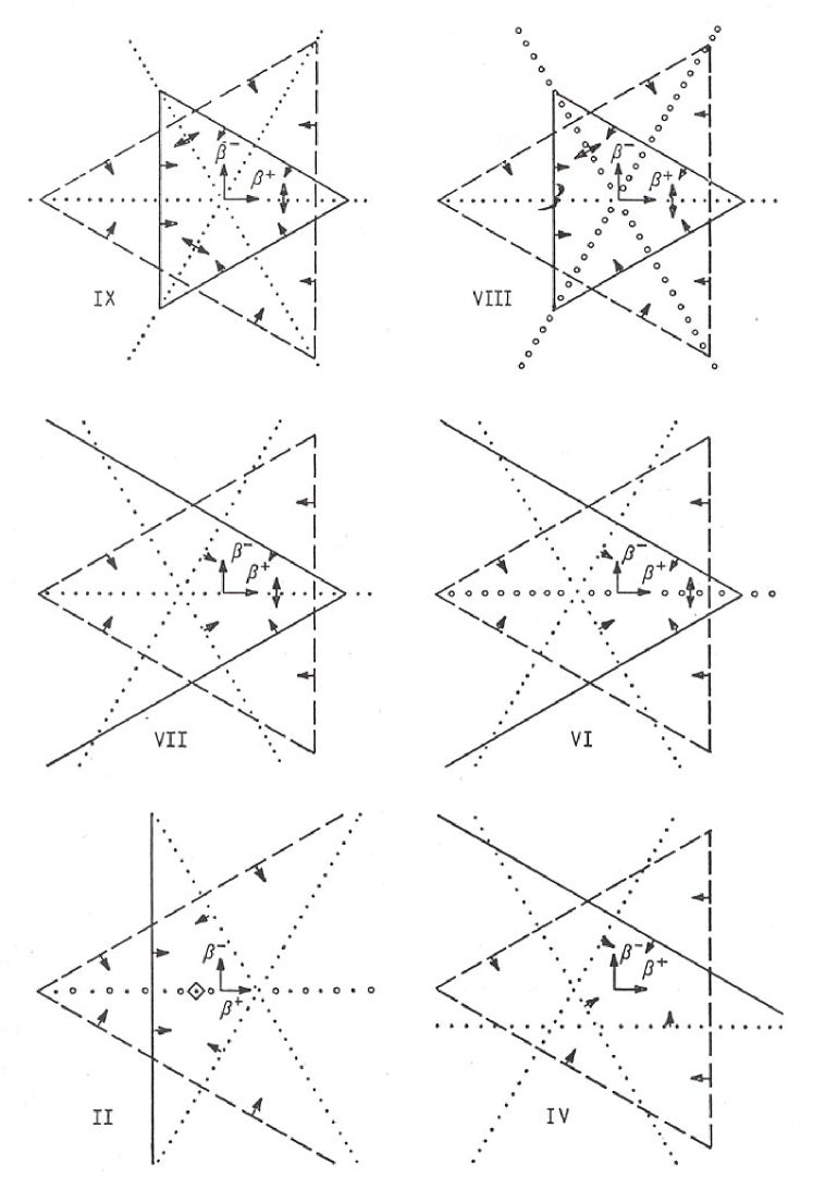
Figure 9: The walls associated with the gravitational, tilt and centrifugal potentials for the canonical points of ${\cal C}_{D}$. Arrows indicate the direction of decreasing values of each potential. Although shown as symmetrical about the origin for simplicity, the tilt and type $(iii)$ centrifugal walls will in general assume unsymmetrical positions. Figure 8 explains the conventions for this figure.

For the canonical points of ${\cal C}_{D}$, the gravitational potential (in supertime time gauge) is closely approximated by the simple time dependent Bianchi type II exponential potential $U_{g}^{(a)}=12n^{(a)\,2}e^{4\beta^{0}-8\beta^{+}_{a}}$ between the positive $\beta^{+}_{b}$- and $\beta^{+}_{c}$-axes and outside the channels. Because of the simple exponential dependence of this potential, a given value of this potential has a constant value of $\beta^{0}-2\beta_{a}^{+}$, i.e. its contours move with velocity $d\beta^{+}_{a}/d\beta^{0}={1\over 2}$ in the flat 3-dimensional spacetime $(diag(3,R),\eta_{AB}d\beta^{A}\otimes d\beta^{B})$. Similarly the tilt potential (in supertime time gauge) in the limit of large anisotropy or extreme tilting along the diagonal axis $e_{a}^{\ \prime}$ is closely approximated by the exponential potential $U^{(a)}_{tilt}=24kle^{2(\beta^{0}+\beta^{+}_{a})}|v_{a}^{\ \prime}|$ between the negative $\beta^{+}_{b}$- and $\beta^{+}_{c}$-axes, and hence its contours move with velocity $d\beta^{+}_{a}/d\beta^{0}=-1$ plus whatever additional velocity is due to the time variation of $v^{\prime}_{a}$ (and $l$ in the class B case). These exponential potentials are indicated by single equipotential lines in Figures 8 and 9, the direction of decreasing values (the direction of the associated force) indicated by arrowheads on these lines. Figure 8 provides a key which indicates the labeling of the various potentials of Figure 9. Although the tilt equipotential locations are shown as symmetrical, decreasing $v_{a}^{\ \prime}$ translates $U^{(a)}_{tilt}$ in the positive $\beta^{+}_{a}$ direction, so that when an individual (primed) component of the fluid current vanishes, the corresponding tilt potential moves out to infinity. A similar statement holds for the exponential gravitational potentials and their dependence on $|n^{(a)}|$. One must actively translate these canonical potentials by the translation (and rescaling) (2.30) to obtain the noncanonical potentials, with Lie algebra contraction causing the potentials to move out to infinity. Equipotential lines of these potentials move with $\beta^{0}$-velocity ${1\over 2}$ in the direction of decreasing values, while the tilt potentials in the exponential regime move with $\beta^{0}$-velocity 1 in the direction of decreasing values neglecting the additional time dependence due to the fluid variables. The centrifugal potentials in supertime time gauge have no explicit dependence on $\beta^{0}$ and hence their motion is entirely due to the $\hat{G}$-angular momentum factor. When this latter factor is constant as occurs in the class A symmetric cases to be described shortly, these potentials are stationary. The type VI and VII potentials in each sector between the negative $\beta^{+}_{b}$- and $\beta^{+}_{c}$-axes, namely $U_{g}(\hbox{VII},n^{(a)}=0)=2|n^{(b)}n^{(c)}|e^{4(\beta^{0}+\beta^{+}_{a})}\hbox{sinh}^{2}2\sqrt{3}(\beta^{-}_{a}-\beta^{-}_{a0})$ and $U_{g}(\hbox{VI},n^{(a)}=0)=2|n^{(b)}n^{(c)}|e^{4(\beta^{0}+\beta^{+}_{a})}\hbox{cosh}^{2}2\sqrt{3}(\beta^{-}_{a}-\beta^{-}_{a0})$ simply translate along the $\beta^{+}_{a}$ axis with velocity $d\beta^{+}_{a}/d\beta^{0}=-1$ in supertime time gauge, so the channels move with unit $\beta^{0}$-velocity in this time gauge (outside their common intersection at semisimple points of ${\cal C}_{D}$).

In the $\beta^{0}$-time gauge, all of the potentials become multiplied by an additional factor of $(-p_{0})^{-1}$, leading to additional implicit time dependence and an additional contribution to the velocities of their contours.

Before discussing the qualititive effect of the various potentials on the dynamics, it is important to have in mind a classification of the specializations which can occur. Because of the existence of various additional continuous (local rotational symmetry and isotropy) and discrete spacetime symmetries, the dynamics admits various special cases where one may consider the phase subspace associated with a submanifold of the configuration space such that initial data in this phase subspace remains in it when evolved by the equations of motion. These special cases are important since they are governed by much simpler systems of differential equations which often admit exact solutions. These exact solutions are the basis of analytic approximation schemes or “diagrammatic solutions”.

Since $Aut_{e}(g)$ is a symmetry group of the equations of motion, any such phase subspaces which are related by the action of an automorphism are equivalent and it suffices to consider only one representative from each equivalence class. These have been described elsewhere for Dirac spinor [42] and perfect fluid [43] sources for the canonical points of ${\cal C}_{D}$ and are summarized for the perfect fluid case in Table 3.

      General case     

                             

    Symmetric cases: g $\in{\cal M}_{S(a)}$ , $v_{b}=v_{c}=0$ class A: all types $(a=1,2,3)$ class B: all types $(a=3)$          Generalized Taub-like cases: g $\in{\cal M}_{GT(a)}$ , $v_{b}=v_{c}$ class A: I $(a=1,2,3)$, V $(a=3)$ class B: V,  VI_h $(a=3)$     

                                                       

    Diagonal case: g $\in{\cal M}_{D}$ class A: all types; $v_{a}=0$ class B: type V; $v_{1}=v_{2}=0$          Taublike symmetric cases: g $\in{\cal M}_{TS(a)}\ ,\ v_{b}=v_{c}=0$ class A: type VI${}_{0}\ (a=3)$ , type I $(a=1,2,3)$ class B: types VI_h,V $(a=3)$     

                                                      

    Taublike cases: g $\in{\cal M}_{T(a)}$ class A: $\{\vbox{\vbox{\hbox{types IX, I $(a=1,2,3)$} \hbox{others $(a=3)$}}}\}$; $v_{1}=v_{2}=v_{3}=0$ class B: $\{\vbox{\vbox{\hbox{types VII${}_{h}$, V $(a=3)$; $v_{1}=v_{2}=0$}\hbox{type III$\equiv$VI${}_{-1}\ (a=2)$; $v_{1}=v_{2}=v_{3}=0$}}}\}$     

 

    Isotropic case: g $\in{\cal M}_{I}$, $v_{a}=0$ class A: types IX, VII₀, I class B: types VII_h, V     

Table 3: Specialization diagram for the perfect fluid dynamics at the canonical points of ${\cal C}_{D}$ , letting $(a,b,c)$ be a cyclic permutation of $(1,2,3)$ when appropriate. For noncanonical points of ${\cal C}_{D}$ , the submanifolds analogous to ${\cal M}_{T(a)}$, ${\cal M}_{TS(a)}$, and ${\cal M}_{GT(a)}$ are characterized by the condition (3.20) rather than $\beta^{-}_{a}=0$ . For noncanonical class A points of ${\cal C}_{D}$ , the type VI₀ Taublike symmetric cases occur for the index value coinciding with the index associated with the vanishing diagonal component of n and the Taublike cases occur for the index $a$ such that $n^{(b)}$ and $n^{(c)}$ are of the same sign or both vanish. The manifold analogous to the isotropic submanifold is obtained by applying to ${\cal M}_{I}$ the diagonal transformation which transforms the canonical point into the given noncanonical point of ${\cal C}_{D}$.

For types I and IX all symmetric and Taublike cases (and for type I all Taublike symmetric cases) are equivalent, while only two inequivalent symmetric cases exist for the remaining class A types. The existence of nontrivial continuous isotropy subgroups of the action of $Aut_{e}(g)$ on ${\cal M}$ for types I, II and V leads to the following additional equivalences for perfect fluid sources. For type I the general case is equivalent to the diagonal case. For types II and V the symmetric case ${\cal M}_{S(3)}$ is equivalent to the diagonal case, while the Taublike type V case is equivalent to the isotropic case when $v_{3}=0$. All Taublike cases except for Bianchi types VI₀ and VI_h are associated with local rotational symmetry and all isotropic cases with spatial isotropy. There also exist equivalences between different Bianchi types [42]. The type VII₀ and type I Taublike cases are equivalent, as are the type VII_h and type V Taublike cases. The symmetric cases correspond to the situation in which the $\hat{G}$-angular momentum is aligned with one of the body-fixed axes, i.e. ${\tilde{P}}_{a}$ has only one nonvanishing component (a class A constant of the motion); this preferred body-fixed axis coincides with one of the space-fixed axes and is a Kasner axis. The remaining two Kasner axes move in the plane orthogonal to this axis. The diagonal case corresponds to vanishing angular momentum, in which case the frame $e=e^{\prime}$ is a Kasner frame. The general case is characterized by the fact that the $\hat{G}$-angular momentum is not aligned with any of the body-fixed axes so that the Kasner axes are distinct from the body-fixed axes.

For the class B case, certain cases are characterized by the vanishing of the nonpotential force, so that the system becomes an ordinary Hamiltonian system. The symmetric case submanifold ${\cal M}_{S(3)}$ is described by the conditions $\theta^{1}=\theta^{2}=0$ in terms of the combined parametrization (3.1) and (3.7). The restriction of ${\tilde{W}}{}^{a}$ to this submanifold is simply ${\tilde{W}}{}^{a}\bigm{|}_{S(3)}=\delta^{a}{}_{3}d\theta^{3}$, using an obvious abbreviated notation for the restriction, so the restriction of the nonpotential force is

 

$${Q\bigm{|}_{S(3)}}$$

 

For this symmetric case the fluid must satisfy $v_{1}=v_{2}=0$ or equivalently $v_{1}^{\ \prime}=v_{2}^{\ \prime}=0$. For type V, one has $e^{\alpha^{3}}=0$ and $Q\bigm{|}_{S(3)}$ is proportional to $d\beta^{+}$; when $v_{3}=0$, the third supermomentum constraint becomes ${\dot{\beta}}{}^{+}=0$ and the constant value of $\beta^{+}$ may be transformed to zero by the action of an automorphism, leaving an ordinary Hamiltonian system in the remaining degrees of freedom. (This case is equivalent to the diagonal case.) The Taublike type VII_h case, being equivalent to the Taublike type V case, is also Hamiltonian. $(\overline{{\cal G}}_{33}=0.)$ For type VI_h (or type V) the Taublike symmetric case is described by the additional condition $d\overline{{\cal G}}_{33}=0$ (namely (3.18) which is equivalent to $n^{a}{}_{a}=0\ ^{(14)}$) or $e^{-\alpha^{3}}n^{(1)}e^{2\sqrt{3}\beta^{-}}=-e^{-\alpha^{3}}n^{(2)}e^{-2\sqrt{3}\beta^{-}}=e^{-\alpha^{3}}q$, where $q$ is defined by the two conditions $q^{2}=-n^{(1)}n^{(2)}$ and $\hbox{sgn}\,q=\hbox{sgn}\,n^{(1)}$, so that $\overline{{\cal G}}_{33}=e^{-2\alpha^{3}}q^{2}$ and the restriction of the nonpotential force to the Taublike symmetric case configuration space is

$$Q\bigm{|}_{TS(3)}=-4a^{2}e^{\beta^{0}+4\beta^{+}}d\ln u\ ,\qquad\ln u\equiv-6\beta^{+}-2\lambda qe^{-\alpha^{3}}\theta^{3}\ ,$$

while the third supermomentum constraint becomes

$${\cal H}^{G}_{3}\bigm{|}_{TS(3)}=2ae^{2(\beta^{0}+\beta^{+})}(\ln u)\dot{\ }=2klv_{3}\ .$$

When $v_{3}=0$, then this constraint requires one to restrict the Taublike symmetric case configuration space by the condition $du=0$, leading to the vanishing of the nonpotential force and an ordinary Hamiltonian system. Setting $q=0$ gives the type V limit which is again equivalent to the diagonal case.

The Taublike symmetric case ${\cal M}_{ST(3)}$ is diagonalized by the following linear transformation AB, which transforms the structure constant tensor out of the space ${\cal C}_{D}$ except for type V $(q=0)$

 

$${\kern-0.24994pt\hbox{$\kappa$}\kern-5.76158pt\kern 0.50003pt\hbox{$\kappa$}\kern-5.76158pt\kern-0.24994pt\raise 0.43304pt\hbox{$\kappa$}_{3}}$$

 

The generalized Taublike case ${\cal M}_{GT(3)}$ is mapped onto the symmetric case ${\cal M}_{S(1)}$ by this linear transformation. The spatial frame $\overline{e}$ is a Kasner frame consisting of eigenvectors of the spatial Ricci curvature.

When $v_{3}=0$, then $u=-3(\beta^{+}+\lambda\sqrt{3}\overline{\beta}{}^{-})$ has a constant value which may be transformed to zero by a translation in $\theta^{3}$. For Bianchi type III $=$ VI_-1, $\lambda=\hbox{sgn}\,n^{(1)}=\pm 1$ holds and $u=5\overline{\beta}{}^{-}_{2}\quad(\lambda=1)$ or $u=-6\overline{\beta}{}^{-}_{2}\quad(\lambda=-1)$ and one has a Taublike case ${\cal M}_{T(2)}$ (i.e. $\overline{\beta}{}^{-}_{2}=0$) or ${\cal M}_{T(1)}$ (i.e. $\overline{\beta}{}^{-}_{1}=0$) respectively when referred to the barred frame. This Taublike case for Bianchi type III is exactly the case where the fourth linearly independent Killing vector field which exists for all spatial metrics of this type [10] becomes a spacetime Killing vector field, leading to local rotational symmetry. Since the (positive curvature) Kantowski-Sachs metrics are related to these by a simple analytic continuation in a particular coordinate system, as discussed in appendix D, the Kantowski-Sachs case is also Hamiltonian.

4 Qualitative Considerations

With the machinery that has been developed in the preceding sections, one can qualitatively or numerically study the time evolution of the general spatially homogeneous perfect fluid spacetime. Three regimes in this evolution are of particular interest, namely the limit $\beta^{0}\to-\infty$ towards the initial singularity in the class of initially expanding models ($p_{0}<0$ as $\beta^{0}\to-\infty$), the limit $\beta^{0}\to\infty$ away from this singularity in the same class of models [38] (omitting the Bianchi type IX subclass, which reach a maximum of $\beta^{0}$ and recollapse) and the small anisotropy limit in the subclass of models which are compatible with spatial isotropy [63] The first regime is especially simple to treat qualitatively, the key ideas for which will now be sketched.

Lifshitz and Khalatnikov, later joined by Belinsky, were led to the qualitative study of spatially homogeneous models by their investigation of the nature of a generic initial cosmological singularity. It seems that the approach to the singularity in adapted comoving coordinates induces a sort of contraction of the Einstein equations which essentially decouples the evolution of the three-plus-one variables at different spatial points while mimicking the behavior of a particular spatially homogeneous model at any given point. This work is concisely summarized and updated in a recent article by these authors [64]. At about the same time as the main thrust of the BLK work began, Misner approached the problem of the dynamics of spatially homogeneous models from an entirely different point of view, paving the way for Ryan to study the qualitative behavior of the approach to the initial singularity in general Bianchi type IX models. This is the same class of models to which BLK confined most of their attention, the relation between the two approaches being described in ref.(24). The formalism of the present article allows one to extend this work to the general spatially homogeneous model.

In studying the regime $\beta^{0}\to-\infty$, it is convenient to use the variable $\Omega\equiv-\beta^{0}$ which increases towards the singularity. As one approaches the singularity, the “anisotropy” increases and the scale over which the motion of the $\beta^{\pm}$ variables occurs becomes much larger than the one over which the curvature of the valleys and corners associated with the channels of Figure 4 is apparent. The various potentials reduce to time dependent exponential or exponentially cutoff potentials in the positive or negative $\beta^{+}_{a}$-sectors (defined with respect to a shifted origin) which are relevant to each potential (as indicated in Figures 8 and 9). These potentials move with either constant or time varying velocity on the $\beta^{+}\beta^{-}$ plane in supertime time gauge. Because of the sharp rise of an exponential, a given potential has little effect on the motion of the universe point until a “collision” or “bounce” occurs, during which the universe point is significantly affected by the potential and then returns to a state in which that potential has little effect on the motion. Again due to the exponential nature of the potentials, essentially only one potential usually affects the universe point at any given time. When no potential exerts a noticable effect on the universe point, the evolution reduces to the free dynamics whose exact solutions are the Kasner solutions, characterized by straight line motion in the $\beta^{+}\beta^{-}$ plane with unit $\beta^{0}$-velocity (a null curve in the flat 3-dimensional spacetime $diag(3,R)$ ).

Exact solutions also exist for each of the cases in which only one potential is present. These may be viewed as scattering problems and used to relate the asymptotic Kasner solutions before and after the collision with that potential. When the velocity of a given potential is constant and timelike ($\beta^{0}$-velocity less than one), one can always transform to its rest frame where the problem reduces to an ordinary 1-dimensional scattering problem in a fixed potential at constant energy [17]. If the velocity is constant but null, one can transform to null coordinates and solve the problem. Because of the super-Hamiltonian constraint, the system trajectory is always a timelike or null curve in $diag(3,R)$ except near the point of maximum expansion in Bianchi type IX models where the spatial curvature is positive and the trajectory becomes spacelike as it makes the transition from expansion to contraction (see Figure 3 of ref.(17)).

One must also consider the possibility that the system trajectory is affected by one of the channels, although this becomes increasingly less likely as the scale of the $\beta^{\pm}$ motion increases (simply because the width of the channel is fixed). In this case, referred to as the case of small oscillations by BLK and as a mixing bounce by Ryan and others, only a qualitative solution exists for the exit of the universe point from the channel [15,29], apart from a numerical calculation of a particular open channel mixing bounce [5,22]. This case can be complicated by the presence of a centrifugal potential in the channel, as discussed by Chitre and Matzner [65] and others [40].

Misner introduced the extremely useful idea of associating a moving “wall” with each potential by selecting a particular contour line which marks the point at which the potential has a large enough value to significantly affect the motion of the universe point. For a given potential and a given moment of time in supertime time gauge, one can consider the simplified super-Hamiltonian constraint in which only the expansion energy and that potential appear and solve it for $\beta^{wall}$, the value of the particular $\beta^{+}_{a}$ or $\beta^{-}_{a}$ coordinate on which the potential depends at which the constraint is satisfied. This locates the “wall contour” or simply “wall” associated with this potential

$$0=-{\textstyle{1\over 2}}p_{0}^{\ 2}+U(\beta^{wall})\ .$$

This contour is the one at which a turning point of the motion would occur if $U$ were time independent, $p_{0}$ were constant, all other potentials were zero and the motion were orthogonal to the contour. In fact since the terms omitted in the super-Hamiltonian constraint are positive (away from the point of maximum expansion in the type IX case), the “turning point” of the orthogonal component of the motion must occur at a smaller value of the potential, namely before the system point can make contact with the wall contour. (Because of the motion of the walls, the “turning point” may only be an actual turning point in the rest frame of the potential.) However, this gap between the wall and “turning point” is on a scale which is usually much smaller than the scale over which the $\beta^{\pm}$ motion is occurring and so provides a useful marker of where a collision occurs between the potential and the universe point.

Since $p_{0}$ is a constant far from the wall contour during a Kasner phase, the value of the potential at the wall contour remains fixed and the wall contour coincides with a given contour of the potential, thus moving with the same velocity as the potential. However, $p_{0}$ may change during the course of a collision, a decrease in $|p_{0}|$ requiring a decrease in the potential value of the wall contour and causing an additional inward motion of the wall contour towards the universe point. In supertime time gauge, the equation of motion for $|p_{0}|=-p_{0}$ in the expanding phase is given by

 

$${|p_{0}|\dot{\ }}$$

 

Using the definitions of Appendix C, the fluid term inside the brackets of eq.(4.2) may be expressed in the obviously nonnegative form

$$6\gamma(l/u^{\bot})^{\gamma}e^{3\beta^{0}(2-\gamma)}[2-\gamma+{\textstyle{1\over 3}}\gamma\mu^{-2}v^{a}v_{a}]\ .$$

Thus all of the terms inside the brackets of eq.(4.2) are nonnegative (apart from the positive curvature regime at Bianchi type IX points), indicating that $|p_{0}|$ increases with supertime and therefore decreases as $\Omega\to\infty$, except in the vacuum type I case where $|p_{0}|$ is a constant. Note that the equation of motion for $\Omega$ in this time gauge, namely $\dot{\Omega}{}=d\Omega/d{\bar{t}}=p_{0}$, determines $\Omega$-time as a function of supertime; these are affinely related only when $p_{0}$ is a constant.

The walls associated with the various gravitational, centrifugal and tilt potentials and their $\Omega$-velocities are as follows [20,21]

 

$${{}U^{(a)}_{g}={\textstyle{1\over 2}}(n^{(a)})^{2}e^{-8(\beta^{+}_{a}-{1\over 2}\beta^{0})}}$$

 

 

$${{}U^{(a)}_{c}(i/ii)={\textstyle{3\over 2}}{\tilde{P}}{}^{\ 2}_{a}|e^{-2\alpha^{a}}n^{(b)}n^{(c)}|^{-1}[\left(\vbox{\vbox{\hbox{sinh}\hbox{cosh}}}\right)\,2\sqrt{3}(\beta^{-}_{a}-\beta^{-}_{a0})]^{-2}}$$

 

 

$${{}U^{(a)}_{tilt}=24kle^{2(\beta^{0}+\beta^{+}_{a})}|v^{\prime}_{a}|}$$

 

Note that there are two walls symmetrically located about $\beta^{-}_{a}=\beta^{-}_{a0}$ for the centrifugal potentials of type $(i)$ and $(ii)$. (For the latter case these walls coincide when $\zeta=1$ and then disappear for $\zeta>1$.) These pairs are represented in Figures 8 and 9 by single dotted lines at $\beta^{-}_{a}=0$ ($\beta^{-}_{a0}=0$ at the canonical points when well defined). More detailed figures indicating these pairs would generalize Figure 1 of ref.(24). Although these walls move away from each other as $|p_{0}|$ decreases for fixed $\tilde{P}_{a}$, their separation decreases on a scale which expands with $\Omega$ to keep up with the other walls. All of the centrifugal walls move in the direction of decreasing values of the associated potential as $|p_{0}|$ decreases.

Between collisions the universe point has unit $\Omega$-velocity while the gravitational walls have $\Omega$-velocity ${1\over 2}$ and the component of the $\Omega$-velocity of the centrifugal walls associated with the explicit dependence on $\beta^{0}$ is 0, so the universe point will overtake and collide with these walls, the length of Kasner segments of the $\beta^{+}\beta^{-}$ motion increasing with $\Omega$ as $\Omega\to\infty$. The tilt wall on the other hand also moves with unit $\Omega$-velocity between collisions neglecting the additional component of the velocity due to the time dependence of $|v^{\prime}_{a}|$ (and $l$ in the class B case), so the universe point can never catch this wall unless significant changes in its motion occur due to the time dependence of $|p_{0}|$, $|v^{\prime}_{a}|$ and $l$. This means that the tilt potential becomes less and less important as $\Omega\to\infty$, as discussed in detail by Ryan [20,21]. All of the walls for each canonical point of ${\cal C}_{D}$ are shown in Figures 8 and 9.

A bounce from a single curvature potential $U^{(a)}_{g}$ is described by the exact type II diagonal vacuum solution found by Taub [11]; the supertime $\overline{t}$ is affinely related to Taub’s time function (by the factor of 12). Consider the case $a=1$ for comparison with the Lifshitz-Khalatnikov notation; the remaining cases follow by cyclic permutation. The Hamiltonian in supertime time gauge is expressed in terms of the coordinates $\{\beta^{\pm}_{1},p_{1\pm}\}$ by

$$H={\textstyle{1\over 2}}(-p_{0}{}^{2}+p_{1+}{}^{2}+p_{1-}{}^{2})+6(n^{(1)})^{2}e^{4(\beta^{0}-2\beta^{+}_{1})}\ ,$$

which is the Hamiltonian of a relativistic particle (with timelike momentum due to the super-Hamiltonian constraint) in an exponential potential which is moving uniformly in the positive $\beta^{+}_{1}$-direction with constant $\beta^{0}$-velocity of magnitude $v={1\over 2}$. A boost in this direction with $\gamma$-factor $(1-v^{2})^{-{1\over 2}}=2/\sqrt{3}$ transforms the inertial coordinates to the rest frame of the potential [16]

 

$${{}(\overline{\beta}{}^{0},\overline{\beta}{}^{+},\overline{p}_{0},\overline{p}_{1+})=3^{-{1\over 2}}(2\beta^{0}-\beta^{+}_{1},2\beta^{+}_{1}-\beta^{0},2p_{0}+p_{+},2p_{+}+p_{0})}$$

 

The problem therefore reduces to free motion in the $\overline{\beta}{}^{0}\beta^{-}_{1}$ plane and an ordinary 1-dimensional scattering problem in the $\overline{\beta}{}^{+}_{1}$-direction with positive energy ${\cal E}_{0}={1\over 2}(\overline{p}_{0}{}^{2}-p_{1-}{}^{2})\equiv{1\over 2}(\overline{p}^{\infty}_{1+})^{2}$ where $\overline{p}^{\infty}_{1+}>0$ is a constant. The super-Hamiltonian constraint

$$(\dot{\overline{\beta}}{}{}^{+}_{1}){}^{2}+12(n^{(1)})^{2}e^{-4\sqrt{3}\,\overline{\beta}^{+}_{1}}=(\overline{p}^{\infty}_{1+})^{2}$$

may be integrated to obtain $\overline{t}$ as a function of $\overline{\beta}{}^{+}_{1}$; inverting the result yields the solution

 

$${{}(\overline{\beta}{}^{0}({\bar{t}}),\beta^{-}_{1}({\bar{t}}))=(-\overline{p}_{0}{\bar{t}}+\overline{\beta}{}^{0}_{0},p_{1-}{\bar{t}}+(\beta_{1}^{-})_{0})}$$

 

where $\overline{t}_{0}$ is the turnaround time. This solution interpolates between two asymptotic Kasner solutions characterized by the null momenta

$$(p_{0}(\pm\infty),p_{1+}(\pm\infty),p_{1-})=3^{-{1\over 2}}(2\overline{p}_{0}\mp\overline{p}{}^{\infty}_{1+},\pm 2\overline{p}{}^{\infty}_{1+}-\overline{p}_{0},\sqrt{3}p_{1-})$$

The scattering problem is therefore most naturally interpreted as a map of the unit circle in the $p_{+}p_{-}$ plane into itself, which is the result of the Lorentz transformation of ordinary reflection from the static potential in its rest frame.

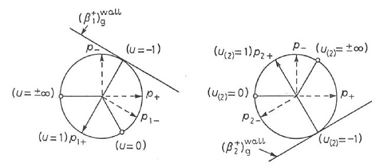
Figure 10: The Lorentz transforms of simple reflection by the gravitational potentials $U^{(1)}$ and $U^{(2)}$ in their rest frames. The asymptotic Kasner states are related by a change of sign of the parameter $u$ in the first case and of $u_{(2)}$ in the second case.

The Lifshitz-Khalatnikov parametrization of the unit circle in the $p_{+}p_{-}$ plane leads to the following representation of the unit momentum coordinates

$$({\hat{p}}_{1+},{\hat{p}}_{1-})={\textstyle{1\over 2}}(1+u+u^{2})^{-1}((1+u)^{2},\sqrt{3}(u^{2}-1))\ ,$$

which enables one to define $u_{\pm\infty}$ for the asymptotic values (4.11) of this unit vector at $\overline{t}=\pm\infty$. The final states with $u_{\infty}\in[1,\infty)$ correspond to initial states with $u\in(-\infty,-1]$; similarly $u_{\infty}\in(0,1]$ corresponds to $u_{-\infty}\in[-1,0)$. No asymptotic states exist with $u=0$ or $u=\pm\infty$ which represent the Lorentz transforms of directions parallel to the equipotential lines of the static potential. Figure 10 illustrates this situation.

Since

$$p_{1-}/|\overline{p}_{0}|=(p_{1-}/|p_{0}|)[2-p_{1+}/|p_{0}|]^{-1}$$

is a constant of the motion, its asymptotic values

$$\hat{\overline{p}}_{1-}(\pm\infty)={\hat{p}}_{1-}(\pm\infty)[2-{\hat{p}}_{1+}(\pm\infty)]^{-1}=3^{-{1\over 2}}(1-u_{\pm\infty}^{\ 2})$$

must coincide, which can only be true if $u_{-\infty}=-u_{\infty}$. ($u_{\infty}=u_{-\infty}$ is ruled out by the case $p_{1-}=0$ of normal incidence.) Thus scattering from the curvature wall $U^{(1)}_{g}$ simply leads to a change of sign of the Lifshitz-Khalatnikov parameter $u_{(1)}=u$. Similarly scattering from the rotated potentials $U^{(2)}_{g}$ and $U^{(3)}_{g}$ leads to a change of sign of the rotated Lifshitz-Khalatnikov parameters $u_{(2)}=P_{231}(u)$ and $u_{(3)}=P_{312}(u)$.

Suppose $u_{\infty}\in[2,\infty)$ and hence $u_{-\infty}\in(-\infty,-2]$, so that the Kasner exponents at $\overline{t}=\infty$ are ordered: $p_{1}(u_{\infty})\leq p_{2}(u_{\infty})\leq p_{3}(u_{\infty})$. The transposition $P_{12}$ then orders the Kasner exponents at ${\bar{t}}=-\infty$ by reflecting the sector $u\in(-\infty,-2]$ across the $p_{+}$-axis into the ordered sector

 

$${{}P_{12}(u_{-\infty})=-(1+u_{-\infty})=u_{\infty}-1}$$

 

Thus the “ordered” Lifshitz-Khalatnikov parameter decreases by 1 in the negative time direction, i.e. as $\Omega$ increases. On the other hand if $u_{\infty}\in[1,2)$, so that $u_{-\infty}\in(-2,-1]$ and the Kasner parameters at ${\bar{t}}=\infty$ are ordered, then the cyclic permutation $P_{312}$ orders the Kasner exponents at ${\bar{t}}=\infty$ by rotating the sector $u\in[-2,-1]$ into the ordered sector

 

$${{}P_{312}(u_{-\infty})=-(1+u_{-\infty})^{-1}=(u_{\infty}-1)^{-1}}$$

 

The “ordered” Lifshitz-Khalatnikov parameter thus decreases by 1, entering the interval [0,1) and then inverts.

The connection between a Lie algebra contraction and an anisotropic singularity may be illustrated by introducing the two special turnaround times defined by ${\bar{t}}{}^{\pm}_{0}=\pm(4\sqrt{3})^{-1}$ $\ln(\sqrt{3}|n^{(1)}|/\overline{p}{}^{\infty}_{1+})$. For ${\bar{t}}_{0}={\bar{t}}{}^{+}_{0}$, the future Kasner limit $\overline{\beta}{}^{+}_{1}({\bar{t}})\to-\overline{p}{}^{\infty}_{1+}{\bar{t}}$ is obtained as ${\bar{t}}\to\infty$; the same asymptotic behavior arises from the contraction $n^{(1)}\to 0$ which sends the turnaround time to $-\infty$. In other words long after the collision the solution approaches the solution for the contracted Bianchi type corresponding to the anisotropic singular scaling $\kern-0.24994pt\hbox{$\beta$}\kern-5.65625pt\kern 0.50003pt\hbox{$\beta$}\kern-5.65625pt\kern-0.24994pt\raise 0.43304pt\hbox{$\beta$}({\bar{t}})\to\kern-0.24994pt\hbox{$\beta$}\kern-5.65625pt\kern 0.50003pt\hbox{$\beta$}\kern-5.65625pt\kern-0.24994pt\raise 0.43304pt\hbox{$\beta$}(\infty)$. Similarly for ${\bar{t}}_{0}={\bar{t}}{}^{-}$, the past Kasner limit $\overline{\beta}{}^{+}_{1}({\bar{t}})\to\overline{p}{}^{\infty}_{1+}{\bar{t}}$ is obtained either as ${\bar{t}}\to-\infty$ or $n^{(1)}\to 0$.

A collision with a single centrifugal potential $U^{(a)}_{c}$ is described by an exact Bianchi type I vacuum solution with nonzero angular momentum, namely the symmetric case ${\cal M}_{S(a)}$. The solution may be found either by transforming the Kasner solutions or by solving the equations of motion. For definiteness consider the case $a=3$. The Hamiltonian in supertime time gauge is

$$H={\textstyle{1\over 2}}(-p_{0}{}^{2}+p_{-}{}^{2}+p_{-}{}^{2})+3\overline{{\cal G}}{}^{-1\,33}{\tilde{P}}_{3}{}^{2}$$

An $S^{1}$-parametrized family of potentials are possible, corresponding to the possible values of $\kern-0.24994pt\hbox{$\kappa$}\kern-5.76158pt\kern 0.50003pt\hbox{$\kappa$}\kern-5.76158pt\kern-0.24994pt\raise 0.43304pt\hbox{$\kappa$}_{3}$ given by (3.4) with $\phi\in[0,2\pi)$. $\tilde{P}_{3}$ is a constant of the motion and since $H$ only depends on $\beta^{-}$, both $\beta^{0}$ and $\beta^{+}$ obey the free dynamics with $p_{0}$ and $p_{+}$ constants of the motion, reducing the problem to a 1-dimensional scattering problem for $\beta^{-}$ with constant energy ${\cal E}_{0}={1\over 2}(p_{0}{}^{2}-p_{+}{}^{2})\equiv(p^{\infty}_{-})^{2}$ and static potential $U^{(3)}_{c}$. The solution may be obtained by integrating the super-Hamiltonian constraint for the supertime as a function of $\beta^{-}$ and then inverting the result (note that supertime and $\Omega$-time are affinely related here).

The following variables make this calculation simple

 

$${{}v=2\sqrt{3}\beta^{-}\,,\quad u^{\pm}=2^{-{1\over 2}}(\cos\phi\,e^{v}\pm\sin\phi\,e^{-v})\,,}$$

 

The solutions $\epsilon=0$ and $\epsilon=-1$ occur only for the type $(ii)$ potential when the energy equals or is greater than, respectively, the maximum value of the potential $U_{max}\equiv{3\over 2}\tilde{P}_{3}{}^{2}|\sin 2\phi|^{-1}$ for this case; the latter solutions pass over the potential barrier while the former ones approach or leave the point of unstable equilibrium $\beta^{-}=\beta^{-}_{0}$. The $\epsilon=1$ bounce solutions are then

 

$${{}|u^{+}|=b\,\hbox{cosh}(24{\cal E}_{0})^{1\over 2}({\bar{t}}-{\bar{t}}_{0})\qquad\quad p_{-}=\pm|2{\cal E}_{0}|^{1\over 2}[1-{\textstyle{3\over 2}}\tilde{P}_{3}/{\cal E}_{0}(u^{-})^{-2}]}$$

 

Note that for a fixed value of $\tilde{P}_{3}$, once ${\cal E}_{0}$ decreases below $U_{max}$, only the bounce solutions are relevant, i.e. for small enough ${\cal E}_{0}$, all three types of potential reverse the orthogonal component of the motion. Similarly as ${\cal E}_{0}$ decreases, the bounce occurs far enough from $\beta^{-}_{0}$ that the potentials $(i)$ and $(ii)$ essentially reduce to pure exponentials.

These solutions have Kasner asymptotes as ${\bar{t}}\to\pm\infty$ which are characterized by the momenta ($p_{0}(\pm\infty)$, $p_{+}(\pm\infty)$, $p_{-}(\pm\infty)$) = ($p_{0}$, $p_{+}$, $\pm p_{-}^{\infty}$) for a bounce solution and ($p_{0}$, $p_{+}$, $p_{-}^{\infty}$) for an $\epsilon=-1$ solution, but $(p_{-}(\infty),p_{-}(-\infty))$ = $(0,p_{-}^{\infty})$ or $(p_{-}^{\infty},0)$ for an $\epsilon=0$ solution. The change in asymptotic momenta associated with the bounce solutions corresponds to reflection across the $p_{-}$-axis.

For this symmetric case one has $(\theta^{1},\theta^{2},\theta^{3})=(0,0,\theta)$ and $\dot{W}{}{}^{a}=\delta^{a}{}_{3}\dot{\theta}$ so from (3.21) one has

 

$${{}\dot{\theta}=6\tilde{P}_{3}\int d{\bar{t}}\,\overline{{\cal G}}{}^{-1\,33}\,,\quad z\equiv\zeta\,\hbox{tanh}\,(24{\cal E})^{1\over 2}({\bar{t}}-{\bar{t}}_{0})\,,\quad\zeta\equiv({\textstyle{2\over 3}}{\cal E}_{0}|\sin 2\phi|(\tilde{P}_{3})^{-2})^{1\over 2}\,,}$$

 

In the compact case $\sin 2\phi>0$, let $\tilde{\theta}\equiv|\sin 2\phi|^{1\over 2}\theta$; since $e^{\theta\kern-0.12251pt\hbox{$\scriptstyle\kappa$}\kern-2.82318pt\kern 0.24503pt\hbox{$\scriptstyle\kappa$}\kern-2.82318pt\kern-0.12251pt\raise 0.21213pt\hbox{$\scriptstyle\kappa$}_{3}}=-\hbox{\bf 1}$ for $\tilde{\theta}=\pi)$, ${\tilde{\theta}}\in[0,\pi)$ represents a closed path in ${\cal M}_{S(3)}$, although twice this interval represents a closed path in $\hat{G}$. Note that for $\zeta\gg 1$, $\tan 2(\tilde{\theta}-\tilde{\theta}_{0})$ begins at a very large negative value at ${\bar{t}}-{\bar{t}}_{0}\to-\infty$ and approaches the sign reversed value at ${\bar{t}}-{\bar{t}}_{0}\to\infty$, so that the total change in $2\tilde{\theta}$ during one bounce is just slightly less that $\pi$. As $\zeta$ decreases the total change in $\tilde{\theta}$ decreases from $\pi/2$ and approaches 0 as $\zeta\to 0$. This is clearly evident in the numerical calculation for the canonical type IX symmetric case ${\cal M}_{S(3)}$ [22], where $\tilde{P}_{3}$ is constant but $|p_{0}|$ and therefore ${\cal E}_{0}$ decreases as $\Omega\to\infty$. In all cases $(\Delta\theta)_{bounce}\to 0$ as $\zeta\to 0$.

The rescaled DeWitt metric on ${\cal M}_{S(3)}$ (set $(\theta^{1},\theta^{2},\theta^{3})=(0,0,\theta)$) is

$$-d\beta^{0}\otimes d\beta^{0}+d\beta^{+}\otimes d\beta^{+}+{}^{2}h\ ,\qquad{}^{2}h=d\beta^{-}\otimes d\beta^{-}+{\textstyle{1\over 6}}\overline{{\cal G}}_{33}d\theta\otimes d\theta\ .$$

The affinely parametrized null geodesics of this metric describe the solutions of the collision with the single potential $U^{(3)}_{c}$ in supertime time gauge. The $\beta^{-}$ scattering problem is then equivalent to finding the geodesics of ${}^{2}h$. This is just the induced metric on the future hyperboloid

$$H_{(2\sqrt{3})^{-1}}=\{(y^{0},y^{1},y^{2})\in R^{3}\bigm{|}(y^{0})^{2}-(y^{1})^{2}-(y^{2})^{2}=(2\sqrt{3})^{-2}\ ,y^{0}>0\}$$

in 3-dimensional Minskowski spacetime with metric $-dy^{0}\otimes dy^{0}+dy^{1}\otimes dy^{1}+dy^{2}\otimes dy^{2}$. Defining

$$(e^{\theta\kern-0.17496pt\hbox{$\kappa$}\kern-4.03311pt\kern 0.35002pt\hbox{$\kappa$}\kern-4.03311pt\kern-0.17496pt\raise 0.30313pt\hbox{$\kappa$}_{3}})^{T}e^{2\beta^{-}\hbox{\bf e}_{-}}e^{\theta\kern-0.17496pt\hbox{$\kappa$}\kern-4.03311pt\kern 0.35002pt\hbox{$\kappa$}\kern-4.03311pt\kern-0.17496pt\raise 0.30313pt\hbox{$\kappa$}_{3}}=(y^{0}+y^{1}){\bf e}^{1}{}_{1}+(y^{0}-y^{1}){\bf e}^{2}{}_{2}-y^{2}({\bf e}^{1}{}_{2}+{\bf e}^{2}{}_{1})+{\bf e}^{3}{}_{3}$$

maps the coordinate surfaces of constant $(\beta^{0},\beta^{+})$ onto $H_{(2\sqrt{3})^{-1}}$. Letting $x\to\theta$ in $(A.4)$ and letting $(c_{3}(2),s_{3}(2))$ be obtained from $(c_{3},s_{3})$ by doubling the argument, and using the double angle identities

$$c_{3}{}^{2}={\textstyle{1\over 2}}(c_{3}(2)+1)\qquad s_{3}{}^{2}=-{\textstyle{1\over 2}}(\tilde{m}{}^{(3)})^{-2}(c_{3}(2)-1)\ ,$$

one obtains explicitly for the case $\tilde{m}{}^{(3)}=(n^{(1)}n^{(2)}))^{1\over 2}\neq 0$ (set $\epsilon=\hbox{sgn}(n^{(1)}n^{(2)})$)

 

$${{}y^{0}+y^{1}=e^{2\sqrt{3}\beta^{-}_{0}}({\textstyle{1\over 2}}[e^{v-v_{0}}-\epsilon e^{-(v-v_{0})}]c_{3}(2)+{\textstyle{1\over 2}}[e^{v-v_{0}}+\epsilon e^{-(v-v_{0})}])\ ,}$$

 

The special linear subgroup $SL(2)_{3}$ acting on ${\cal M}_{S(3)}$ maps onto the action of the 3-dimensional Lorentz group on $H_{(2\sqrt{3})^{-1}}$; the coordinates $\{\beta^{-},\theta\}$ are comoving with respect to the subgroup generated by $\kern-0.24994pt\hbox{$\kappa$}\kern-5.76158pt\kern 0.50003pt\hbox{$\kappa$}\kern-5.76158pt\kern-0.24994pt\raise 0.43304pt\hbox{$\kappa$}_{3}$. This subgroup corresponds to null rotations for $\phi=0,\pi$, rotations in the $y^{1}-y^{2}$ plane for $\phi=\pi/4,5\pi/4$, boosts along $y^{2}$ for $\phi=3\pi/4,7\pi/4$ and combinations of these for other values ($\hbox{\bf e}_{-}$ generates boosts along $y^{1}$).

Geodesics with $\theta=\theta_{0}$ have zero angular momentum with respect to this subgroup, i.e. $\tilde{P}_{3}=0$, and are diagonalized by the constant active transformation $e^{\theta_{0}\kern-0.12251pt\hbox{$\scriptstyle\kappa$}\kern-2.82318pt\kern 0.24503pt\hbox{$\scriptstyle\kappa$}\kern-2.82318pt\kern-0.12251pt\raise 0.21213pt\hbox{$\scriptstyle\kappa$}_{3}}$. However, these geodesics have nonzero angular momentum with respect to the subgroups generated by other values of $\kern-0.24994pt\hbox{$\kappa$}\kern-5.76158pt\kern 0.50003pt\hbox{$\kappa$}\kern-5.76158pt\kern-0.24994pt\raise 0.43304pt\hbox{$\kappa$}_{3}$ (modulo sign). In the canonical type IX or VIII cases, $\theta\to\theta+\theta_{0}$ corresponds to a rotation or boost by the angle or natural boost parameter $2\theta_{0}$ because of the double angle functions. For small angular momentum in the canonical type IX case, a geodesic has $\Delta(2\theta)\sim\pi$ as if the projection to the $y^{1}-y^{2}$ plane were flat, but as the angular momentum increases, the curvature of the hyperboloid decreases this angle.

The classic discussion of Lifshitz and Khalatnikov of an “era” of successive alternating Kasner regimes describes a sequence of bounces between the gravitational wall $U^{(1)}$ in the upper half plane and $U^{(2)}$ in the lower half plane as the universe moves out of the corner where these walls intersect with increasing supertime. Reversing the direction of time in order to approach the initial singularity, as in $\Omega$-time, one must reverse the sign of the momenta; “initial” and “final” will be correlated with this reversed direction of time in the following discussion. An initial Kasner phase with $u^{ordered}=u\in[1,\infty)$ is headed for the wall $\beta^{+}_{1}=(\beta^{+}_{1})^{wall}_{g}$, and then bounces from this wall into the second Kasner phase with $u^{ordered}=u-1$ so that it is headed for the wall $\beta^{+}_{2}=(\beta^{+}_{2})^{wall}_{g}$. It then bounces from this wall into the Kasner phase with $u^{ordered}=u-2$, etc. When $u^{ordered}$ enters the interval $[0,1]$, the final Kasner phase (or “epoch”) heads away from both walls. Figure 10 indicates the scattering problem for each bounce.

This approximation is valid as long as the universe point does not penetrate deep enough into the vertex or corner between the two asymptotic potentials to feel the effects of the channel where the straight line contour approximation of Figure 5 breaks down. When the effect of the channel is important, the regime is called a “long era” or “mixing bounce” and the type VII or VI gravitational potential for an open or closed channel respectively may be used as an approximation for the channels of types VIII and IX outside their common intersection. A qualitative treatment of the exact type VII₀ and VI₀ diagonal vacuum case in this context was first given by Lifshitz and Khalatnikov [26] and then in a better approximation by Khalatnikov and Pokrovsky [29].

The Hamiltonian for this case in supertime time gauge at the canonical points of ${\cal C}_{D}$ is

$$\left(\vbox{\vbox{\hbox{VII${}_{0}$}\hbox{VI${}_{0}$}}}\right):\hskip 30.0ptH={\textstyle{1\over 2}}(-p_{0}{}^{2}+p_{+}{}^{2}+p_{-}{}^{2})+24e^{4(\beta^{0}+\beta^{+})}\left(\vbox{ \vbox{\hbox{$\sinh^{2}2\sqrt{3}\beta^{-}$}\hbox{$\cosh^{2}2\sqrt{3}\beta^{-}$}}}\right)\ .$$

The potential moves with constant $\Omega$-velocity $d\beta^{+}/d\Omega=-1$ (a null velocity in $diag(3,R)$) so a rest frame does not exist and one must instead use null coordinates

 

$${{}(w,v,p_{w},p_{v})=(\beta^{0}+\beta^{+},\beta^{0}-\beta^{+},{\textstyle{1\over 2}}(p_{0}+p_{+}),{\textstyle{1\over 2}}(p_{0}-p_{+}))\ ,}$$

 

The coordinate $w$ comoves with the potential function, while $v$ describes the motion of the system relative to the potential.

The Taublike type VI₀ case with $\beta^{-}=0=p_{-}$ is an exact solution which is useful to consider in detail and represents the path at the center of the closed channel

 

$${{}v-v_{0}-V{\bar{t}}=3p_{v}{}^{-2}e^{4w}={\textstyle{1\over 12}}\xi^{2}\ ,\qquad 0=H=-2p_{v}V\to V=0\ ,}$$

 

The turnaround time ${\bar{t}}_{0}$ is defined by $p_{0}({\bar{t}}_{0})=0$ or $12p_{v}{}^{-2}e^{4w({\bar{t}}_{0})}=1$, while setting ${1\over 2}p_{0}{}^{2}=24e^{4(\beta^{0}+\beta^{+}_{wall})}=24e^{4w_{wall}}$ defines the location of the wall for this $\beta^{-}=0$ case

 

$${{}\beta^{+}_{wall}=\Omega={\textstyle{1\over 2}}\ln[|p_{0}|(4\sqrt{3})^{-1}]\,,\qquad d\beta^{+}_{wall}d\Omega=1-4(1+(12)^{-1}p_{v}{}^{2}e^{4w})^{-2}\,,}$$

 

The system has the past Kasner limit at ${\bar{t}}=-\infty=w$ characterized by the Lifshitz-Khalatnikov parameter $u={1\over 2}$ (free motion in the positive $\beta^{+}$-direction towards the wall), and the Kasner limit at ${\bar{t}}=\infty=w$ characterized by the L-K parameter $u=\infty$ (free motion away from the wall) long after the collision when it has reversed direction and is again moving along a null curve in $diag(3,R)$. The future Kasner limit does not look like free motion in the supertime time gauge since the supertime remains sensitive to the small curvature in this limit and does not reach a stage where it is affinely related to $\Omega$-time and instead diverges from $\Omega$-time.

From the point of view of $\Omega$-time, both the universe point and the wall initially have unit $\Omega$-velocity and hence the universe point cannot overtake the wall. (This is the origin of the term “long era”, since this behavior will persist for a long period of $\Omega$-time.) However, since the universe point and potential have no relative motion, the very small value of the potential at the location of the universe point has a continued effect and over a long time begins to reverse the motion and decrease the expansion energy which in turn slows down the wall enough so that an actual collision occurs at the turnaround point when both the wall and universe point have zero $\Omega$-velocity and the same position, after which the wall resumes its unit $\Omega$-velocity in the same direction and the universe point returns to its unit $\Omega$-velocity but in the opposite direction. Modulo constants this same solution describes a head on collision with the approximate tilt potential $U^{(3)}_{tilt}$ for constant $|v^{\prime}_{3}|$.

By introducing the new time variable $\xi=|6/p_{v}|e^{2w}=|6/p_{v}|e^{2w_{0}+4|p_{v}|{\bar{t}}}$ and the abbreviation $q=4\sqrt{3}\beta^{-}$, the equation of motion for $\beta^{-}$ is given by [29]

$$d^{2}q/d\xi^{2}+\xi^{-1}dq/d\xi+\hbox{sinh}\,q=0\ .$$

For $q\ll 1$ where $\hbox{sinh}\,q\approx q$, this is just Bessel’s equation of order zero [16,26], while for $\xi\gg 1$ (at very late supertime), this has an exact solution in terms of Jacobi elliptic functions [29]. Khalatikov and Pokrovsky use a WKB-like approximation involving this approximate solution to obtain a qualitative solution valid for all times and whose limit at ${\bar{t}}\to-\infty$ specifies the asymptotic Kasner phase which precedes the channel corner run in supertime (but follows it in $\Omega$-time).

Consider the case $\beta^{-}\ll 1$ where the approximation $\hbox{sinh}\,4\sqrt{3}\beta^{-}\approx 4\sqrt{3}\beta^{-}$ is valid and the part of the Hamiltonian which governs the $\beta^{-}$-motion is just that of a harmonic oscillator with the supertime frequency $\omega\equiv 24e^{2w}=4|p_{v}|\xi$

$$H=-p_{w}p_{v}+24e^{4w}\delta^{Z}_{VIII}+H_{-}\qquad H_{-}={\textstyle{1\over 2}}p_{-}{}^{2}+{\textstyle{1\over 2}}\omega^{2}(\beta^{-})^{2}\ .$$

In the adiabatic limit which occurs at late supertime ($\xi\gg 1$) when the change in frequency per period of ocsillation goes to zero, one has the approximate solution

 

$${\beta^{-}}$$

 

where the expression for the amplitude follows from the constancy of the adiabatic invariant $H_{-}/\omega={1\over 2}A^{2}\omega=b$, as discussed by Misner [15]. The constant $C$ is the constant introduced by Khalatnikov and Pokrovsky [29].

The equation of motion for $v$ may be averaged, using $\langle(\beta^{-})^{2}\rangle={1\over 2}A^{2}$

 

$${{}\ddot{v}=192e^{4w}\delta^{Z}_{VIII}+(48)^{2}e^{4w}(\beta^{-})^{2}\ ,\qquad\langle\ddot{v}\rangle=192e^{4w}\delta^{Z}_{VIII}+96be^{2w}\ ,}$$

 

The averaged super-Hamiltonian constraint requires $V=0$. Note that the leading approximation to the $(w,v)$ motion in the closed channel case is just the Taublike type VI₀ vacuum solution.

At early $\Omega$-time, the universe point in its initial asymptotic Kasner phase and the potential both have unit $\Omega$-velocity and keep pace with each other, so $w=\beta^{+}-\Omega$ changes only slowly in $\Omega$-time. (Supertime and $\Omega$-time diverge at ${\bar{t}}\to\infty$.) As the frequency decreases with increasing $\Omega$-time, the amplitude increases and the $\beta^{+}$ motion slows down relative to the potential until the small $\beta$ approximation breaks down, eventually reversing its direction, and after a final bounce goes into an asymptotic Kasner phase which leaves the channel potential behind.

One can also consider a mixing bounce with a centrifugal wall present in the channel. This corresponds to the Bianchi type VII₀ or VI₀ symmetric case ${\cal M}_{S(3)}$. Adding the term $3{\tilde{P}}_{3}{}^{2}\overline{{\cal G}}{}^{-1\,33}$ to (4.24) only effects the $\beta^{-}$ motion directly, while the constant $\tilde{P}_{3}$ enables one to find the variable $\theta$ defined as in (4.18). Matzner and Chitre [65] discuss this case in the adiabatic limit for $\beta^{-}\ll 1$. The mixing bounce is confined to the region between the channel gravitational wall and one centrifugal wall in the open channel case where the $\beta^{-}$ motion corresponds to a 2-dimensional oscillator with nonzero angular momentum. In the closed channel case the situation is much different.

When the curvature of the channel is not important, one simply has a sequence of bounces between one gravitational wall and a centrifugal wall. During the bounces from the latter wall the ordered Lifshitz-Khalatnikov parameter $u^{ordered}$ does not change. Such a sequence of bounces with an exponential centrifugal wall is described in terms of transformations of the first and second type in ref.(24).

The importance of the $a^{2}$ scalar curvature term on the dynamics also can be described by a wall

 

$${{}U^{classB}_{g}=72a^{2}e^{4(\beta^{0}+\beta^{+})}\ ,}$$

 

This potential becomes important only during collisions with its associated wall, but since this wall has unit $\Omega$-velocity away from the location of the universe point when it is in free motion, it becomes less and less important as $\Omega\to\infty$. The exact diagonal Bianchi type V solution describes a collision with this wall

$$H={\textstyle{1\over 2}}(-p_{0}{}^{2}+p_{+}{}^{2}+p_{-}{}^{2})+{\textstyle{1\over 2}}(12a)^{2}e^{4(\beta^{0}+\beta^{+})}\ .$$

$\beta^{\pm}$ obey the free equations of motion (since $V^{\ast}=0$) with constant $p_{\pm}$, leaving the super-Hamiltonian constraint to determine $\beta^{0}$. This is easily integrated if one imposes the supermomentum constraint $p_{+}=0$, thus setting $\beta^{+}=\beta^{+}_{0}$. (The equations of motion for $p_{+}\neq 0$ are integrable in null coordinates, but the super-Hamiltonian constraint then forces $p_{+}=0$.)

 

$${{}\beta^{-}=p_{-}({\bar{t}}-{\bar{t}}_{0})+\beta^{-}_{0}\ ,\qquad\dot{\beta}{}{}^{0\,2}-(12a)^{2}e^{4(\beta^{0}+\beta^{+}_{0})}=p_{-}{}^{2}\ ,}$$

 

The evolution of $\beta^{0}$ corresponds to motion in the 1-dimensional potential
$-{1\over 2}(12a)^{2}e^{4(\beta^{0}+\beta^{+})}$ with constant energy ${\cal E}_{0}={1\over 2}p_{-}{}^{2}$. The expanding solution has ${\bar{t}}-{\bar{t}}_{0}\in(-\infty,0)$; at ${\bar{t}}\to-\infty$ the solution has a Kasner limit but it runs out of supertime at ${\bar{t}}={\bar{t}}_{0}$ when a collision takes place. The wall moves in from $\beta^{+}=\infty$ at ${\bar{t}}=-\infty$ when it has unit $\Omega$-velocity to $\beta^{+}=\beta^{+}_{0}$ where its velocity vanishes and the wall makes contact with the universe point at a finite value of $\beta^{-}$. However, the proper time goes to $\infty$ at ${\bar{t}}={\bar{t}}_{0}$ since near ${\bar{t}}\approx{\bar{t}}_{0}$

$$t-t_{0}=\int e^{3\beta^{0}}d{\bar{t}}\sim\int|{\bar{t}}-{\bar{t}}_{0}|^{-{3\over 2}}d{\bar{t}}\sim|{\bar{t}}-{\bar{t}}_{0}|^{-{1\over 2}}\ .$$

Thus even though $\beta^{-}$ obeys the free dynamics in supertime time gauge, it runs out of supertime at a finite value $\beta^{-}_{0}$, i.e. its value becomes frozen in proper time or $\Omega$-time.

It is basically an effect of this kind which seems to result in isotropization of type VII_h models with “frozen in” values of $\beta^{-}$ as $\beta^{0}\to\infty$ [40]. A similar effect occurs for all Bianchi types when the matter contributions to the Hamiltonian dominate the dynamics as $\beta^{0}\to\infty$, as noted by Doroshkevich, Lukash and Novikov [40]. For example, consider the exact diagonal type I case where $v_{a}=0=P_{a}$ and the Hamiltonian is

$$H={\textstyle{1\over 2}}(-p_{0}{}^{2}+p_{+}{}^{2}+p_{-}{}^{2})+12e^{3\beta^{0}}{\cal H}_{M}\,,\qquad 12e^{3\beta^{0}}{\cal H}_{M}=24kl^{\gamma}e^{3\beta^{0}(2-\gamma)}\ .$$

Here $p_{\pm}$ are constants and $\beta^{\pm}$ undergo free motion, reducing problem of the evolution of $\beta^{0}$ to motion in the potential $-24kl^{\gamma}e^{3\beta^{0}(2-\gamma)}$ with constant energy ${\cal E}_{0}={1\over 2}(p_{+}{}^{2}+p_{-}{}^{2})$. One may directly integrate the super-Hamiltonian constraint

 

$${{}{\textstyle{1\over 2}}(\dot{\beta}{}{}^{0})^{2}-24kl^{\gamma}e^{3\beta^{0}(2-\gamma)}={\cal E}_{0}\ ,}$$

 

The growth of the matter Hamiltonian as $\beta^{0}\to\infty$ again leads to a singularity in supertime and hence a “freezing in” of the values of $\beta^{\pm}$ occurs in proper time or $\Omega$-time when $\gamma\neq 2$. However, these effects are important for the direction $\beta^{0}\to\infty$ but diminish in importance as $\Omega\to\infty$, since the solution quickly approaches its Kasner asymptote.

On the other hand when $\gamma=2$, the system again experiences free motion but along a timelike direction in $diag(3,R)$

$$\eta^{AB}p_{A}p_{B}=-48kl^{2}\,,\quad d\beta/d\Omega=[(d\beta^{+}/d\Omega)^{2}+(d\beta^{-}/d\Omega)^{2}]^{1\over 2}=[1-48kl^{2}p_{0}{}^{-2}]^{1\over 2}\ .$$

A stiff perfect fluid with $v_{a}=0$ only changes the supertime time gauge Hamiltonian by the addition of a positive constant; the only change one must make in the description of a collision with a gravitational or centrifugal wall is ${\cal E}_{0}\to{\cal E}_{0}+24kl^{2}$, where ${\cal E}_{0}$ is the constant energy defined in each of these problems. (It is exactly this change which allows one to easily insert a stiff perfect fluid in the Taub-Nut spacetime [41].) Collisions with gravitational walls as $\Omega\to\infty$ decrease $|p_{0}|$ and therefore reduce the $\Omega$-velocity of the universe point between collisions. If the universe point does not escape from the gravitational walls first, then eventually one has $d\beta/d\Omega<{1\over 2}$ , after which the universe point can no longer catch the faster moving gravitational walls and remains in this free motion phase as $\Omega\to\infty$. Thus such a stiff perfect fluid (or scalar field [66]) leads to an end of an “oscillatory approach to the initial singularity”. (See below.) Similar calculations may be used to study the effect of a nonzero cosmological constant which only directly affects the equation of motion of $\beta^{0}$ and then indirectly affects the remaining variables through the appearance of $\beta^{0}$ in their equations of motion [67].

What has been described so far are exact or qualitative solutions for the case in which only one or two potentials in the supertime time gauge Hamiltonian play an important role at any given time. The importance of a given potential is described by a collision of the universe point with the wall associated with that potential or with a corner where two walls meet and a more careful description may be required. Each such phase of the motion is preceded and followed by asymptotic Kasner phases which are related to each other by the exact or qualitative solution for that collision. Each collision is therefore interpreted as a scattering problem. As $\Omega\to\infty$ one quickly reaches a stage in which the description in terms of successive collisions with different walls is valid and one may approximate the evolution by matching together the Kasner asymptotes between collisions.

The class A diagonal case is easiest to describe in this manner. As (4.36) shows, the matter potential is exponentially cutoff as $\Omega\to\infty$ and even when it dominates the spatial curvature, (4.37) shows that it has a very shortlived effect as $\Omega\to\infty$, i.e. “the matter is dynamically unimportant” as $\Omega\to\infty$. In this limit the system obeys the vacuum dynamics, leaving only the gravitational walls to determine the qualitative solution. Since these walls move with $\Omega$-velocity $1\over 2$ between collisions while the universe point moves with unit $\Omega$-velocity, in the semisimple case of Bianchi types VIII and IX where these walls form closed trapping regions, the collisions never stop, leading to an “oscillatory approach to the initial singularity” in the words of Lifshitz, Khalatnikov and Belinsky. The oscillations occur in the values of the variables $e^{\beta^{1}}$, $e^{\beta^{2}}$ and $e^{\beta^{3}}$, a half period of an oscillation corresponding to two Kasner phases (“Kasner epochs” [24]) joined by a collision at the maximum or minimum point. A single excursion of the universe point into the vertex between two walls is called a Kasner era. Except for collisions with corners between two walls, these two types experience the same motion. However, as $\Omega\to\infty$ the size of the corner region where channel effects are important becomes increasingly smaller in relation to the triangular trapping region. For types VI₀ and VII₀ the missing third wall provides an escape route which leads to only a single Kasner era before the system enters a final Kasner phase as $\Omega\to\infty$, while for type II only one collision with the single gravitational wall occurs between two asymptotic Kasner epochs. The Taublike cases for types VI₀, VIII and IX are special cases characterized by channel trajectories which undergo a single collision with one gravitational wall followed by an escape down an open channel in the semisimple case, while the isotropic cases have no $\beta^{\pm}$ motion at all. The type IX isotropic case is exceptional in that the matter is always dynamically important since the positive spatial curvature makes the vacuum super-Hamiltonian negative-definite. The Kasner axes for the diagonal case coincide with the body-fixed and space-fixed axes and are eigendirections of the spatial Ricci curvature tensor.

The symmetric cases (“nontumbling models” [68]) are much easier to describe qualitatively than the general case since the $\hat{G}$-angular momentum $\tilde{P}_{a}$ is aligned with one of the diagonal axes which is in fact an eigendirection of the spatial Ricci curvature in all instances. This axis is also an eigendirection of both g and K, so it is a Kasner axis. Only the 1-parameter subgroup of $\hat{G}$ which leaves this preferred axis invariant is relevant to the dynamics; for this subgroup $\tilde{P}_{a}$ and $P_{a}$ coincide and have a single nonvanishing component. The same is true of $v_{a}^{\prime}$ and $v_{a}$ and of the components of the supermomentum $P^{\prime}(\kern-0.24994pt\hbox{$\delta$}\kern-4.44444pt\kern 0.50003pt\hbox{$\delta$}\kern-4.44444pt\kern-0.24994pt\raise 0.43304pt\hbox{$\delta$}_{a})$ and $P(\kern-0.24994pt\hbox{$\delta$}\kern-4.44444pt\kern 0.50003pt\hbox{$\delta$}\kern-4.44444pt\kern-0.24994pt\raise 0.43304pt\hbox{$\delta$}_{a})$ with respect to the primed and unprimed frames, all of which have a single (possibly) nonvanishing component along the preferred axis. For the symmetric case ${\cal M}_{S(a)}$, the index $a$ is associated with this preferred axis; as usual let $(a,b,c)$ be the associated cyclic permutation of $(1,2,3)$. (Because of the block diagonal form of g and K, the remaining two Kasner axes are linear combinations of $e_{b}$ and $e_{c}$.) Then $v_{a}=v_{a}^{\prime}$ is a constant. In the class A case excluding the degenerate types I and II, $a$ may assume any value and $l$ and $\tilde{P}_{a}=P_{a}$ are constants such that $e^{\alpha^{a}}{\tilde{P}}_{a}=-2klv^{\prime}_{a}$, leading to a single nonzero centrifugal potential which is static in supertime time gauge. In the class B case, only $a=3$ is allowed and $e^{\alpha^{3}}{\tilde{P}}_{3}+ap_{+}=-2klv^{\prime}_{3}$, but neither $\tilde{P}_{3}$ nor $l$ is a constant and the centrifugal potential is not static.

For the case $n^{(a)}\neq 0$ and $\hbox{rank {\bf n}}\,>1$, the walls associated with the gravitational potentials and the single centrifugal potential define closed trapping regions as is easily seen from Figure 9. For the type $(ii)$ centrifugal potential, the pair of walls do not come into existence until $\zeta\leq 1$ (see (4.3)) but since $|p_{0}|$ decreases towards zero as $\Omega\to\infty$, this condition is eventually satisfied (unless $|p_{0}|$ has a limit away from zero as may occur in the case of a stiff perfect fluid). In the class A case one may describe the $\Omega\to\infty$ evolution in terms of collisions with the centrifugal wall and the gravitational walls between regimes of free motion. Since these walls move with $\Omega$-velocity 0 and $1\over 2$ respectively between collisions, while the universe point moves with unit $\Omega$-velocity, in the case where closed trapping regions exist the collisions never stop, leading to an “oscillatory approach to the initial singularity”. In this case one must make a distinction between a Kasner epoch and an ordinary epoch. An ordinary epoch refers to a period of free motion in the $\beta^{+}\beta^{-}$ plane, while a Kasner epoch refers to a period of free motion with respect to the full rescaled DeWitt metric which includes collisions with centrifugal walls. In the latter case one can always transform away the constant $\hat{G}$-angular momentum $P_{a}$ by a constant linear transformation from the space-fixed axes $e_{b}$ and $e_{c}$ to the Kasner axes. Since the Kasner axes are time independent in a period of free motion, they can change only during collisions with gravitational walls.

As $|p_{0}|$ decreases due to collisions with gravitational walls, the single centrifugal wall moves outward toward decreasing values of the centrifugal potential where the type $(i)$ and $(ii)$ potentials rapidly approach the asymptotic exponential potentials of type $(iii)$ and the distinction between the three types of centrifugal potentials becomes unimportant. Note also that the value of $\overline{{\cal G}}{}^{-1aa}$ at the universe point experiences local maxima at each collision with the corresponding centrifugal wall and these local maxima approach zero as the wall moves out. Since $\overline{{\cal G}}{}^{-1aa}$ goes to zero and since $\tilde{P}_{a}$ is a constant in the class A symmetric case ${\cal M}_{D}$, the offdiagonal velocity $\dot{W}{}{}^{a}=6\overline{{\cal G}}{}^{-1aa}\tilde{P}_{a}$ also goes to zero. The single nonvanishing automorphism variable $\theta$ is given by the integral of $\dot{W}{}{}^{a}$. Because $\overline{{\cal G}}{}^{-1aa}$ is exponentially cutoff, $\theta$ essentially changes only during a collision with the centrifugal wall where the value of $\overline{{\cal G}}{}^{-1aa}$ at the universe point assumes a local maximum which decreases with each collision. The discussion of (4.18) in fact shows that the total change $(\Delta\theta)_{bounce}$ of this variable during a single collision approaches zero as $|p_{0}|\to 0$. An argument due to Lifshitz, Khalatnikov and Belinsky [26] shows that the sum of these changes from any given time as $\Omega\to\infty$ is finite, so $\theta$ approaches a limiting value $\theta_{0}$ as $\Omega\to\infty$.

If $n^{(a)}=0$, then the universe point bounces around between the centrifugal wall and a gravitational wall until it eventually enters a final Kasner phase which leaves both walls behind forever as $\Omega\to\infty$. In the type VIII case with a type $(ii)$ centrifugal potential, the universe point will collide with the gravitational walls until $|p_{0}|$ is lowered enough for the pair of centrifugal walls to come into existence, after which the motion will be confined to a smaller trapping region. Similarly in the type VI₀ symmetric case with a type $(ii)$ centrifugal potential (associated with ${\cal M}_{S(3)}$ in the canonical case), it is possible that a final Kasner phase is reached before the centrifugal walls appear.

Consider the analogy with the central force problem. If one imagines a nonrelativistic particle in free motion on $R^{3}$ whose radial motion is continually reversed at large distances from the origin by collisions with an expanding spherical shell centered at the origin, the angular momentum will be conserved but the impact vector connecting the origin to the point of closest approach of the particle to the origin will change at each collision. A different translation of the origin will then be required in each free motion phase between collisions to transform away the angular momentum. The Kasner axes are changed by collisions with the gravitational walls for a similar reason. Thus even after the motion in the offdiagonal variable $\theta$ essentially stops and one transforms to a diagonal gauge frame where its limiting value $\theta_{0}$ is zero (so that $e_{d}=e_{d}^{\prime}$), two of the Kasner axes do not coincide with the diagonal axes (otherwise the $\hat{G}$-angular momentum would be zero) and continue to change at each collision with a gravitational wall.

As long as the $a^{2}$-curvature potential is important in the class B case, this description is not valid since the system will not experience free motion between collisions with the walls and the analytic description of an individual collision given above will not be valid. However, eventually this curvature potential becomes unimportant as $\Omega\to\infty$ as indicated by the above wall description and the evolution reduces to that of the corresponding class A model with one important exception. Only the symmetric case ${\cal M}_{S(3)}$ is allowed and it is not the $\hat{G}$-angular momentum $\tilde{P}_{3}=P_{3}$ which is a constant for the vacuum dynamics but rather the supermomentum $e^{\alpha^{3}}{\tilde{P}}_{3}+ap_{+}$. The equation of motion for $\tilde{P}_{3}$ in this case, namely $({\tilde{P}}_{3})\dot{\ }=NQ_{3}=48ae^{4(\beta^{0}+\beta^{+})}e^{\alpha^{3}}\overline{{\cal G}}_{33}$, is exactly $-ae^{-\alpha^{3}}$ times the equation of motion for $p_{+}$ (excluding the degenerate type V case), so even in the limit that the $a^{2}$ curvature potential is unimportant, $\tilde{P}_{3}$ still changes during collisions with gravitational walls to compensate for the change in $p_{+}$ which occurs during these collisions, causing additional motion of the centrifugal wall. This additional change in the $\hat{G}$-angular momentum compared to the corresponding class A case then leads to an additional change in the Kasner axes relative to that case. Also since $n^{(3)}=0$ for the class B case, closed trapping zones do not occur and a final Kasner phase exists as $\Omega\to\infty$ when the universe eventually leaves the walls behind.

This discussion has assumed that the matter is not dynamically important as in the diagonal case (when $\gamma\neq 2$). The fluid variable $n$ may be expressed in the form $n=e^{3\Omega}l/u^{\bot}$ where $u^{\bot}\geq 1$. In the class A case $l$ is a constant; for given values of $l$ and $\Omega$, $n$ can only be less than its corresponding value in the diagonal case where $u^{\bot}=1$ since $v_{a}\neq 0$ implies $u^{\bot}>1$. A similar statement holds for $\mu$ and $p$. This means that the only difference the nonzero value of $v_{a}$ can make that might lead to the dynamical importance of matter in the symmetric case ${\cal M}_{S(3)}$ would be if $u^{\bot}\gg 1$. In this case the matter super-Hamiltonian is approximated by the exponential tilt potential $U^{(a)}_{tilt}$, but since $v_{a}$ is a constant, the associated tilt wall moves out with unit $\Omega$-velocity between collisions of the universe point with the gravitational walls and becomes increasingly less important as $\Omega\to\infty$. In this limit one is justified in ignoring the matter potentials. However, the constant nonzero value of the fluid supermomentum is required to allow a nonvanishing centrifugal potential (when the symmetric case is nontrivial, i.e. not equivalent to a diagonal case).

In the class B case, $l$ is not constant but satisfies the equation of motion $(\ln l)\dot{\ }=24ae^{\beta^{0}+4\beta^{+}}v_{3}/v^{\bot}$, so this argument does not go through. Because of the supermomentum constraint, $l$ must approach a constant as $\Omega\to\infty$ if the gravitational supermomentum is to approach a constant as assumed above. In fact since the equation of motion for the supermomentum constraint is $(2klv_{3})\dot{\ }=(e^{\alpha^{3}}+ap_{+})\dot{\ }=a\{p_{+},{\cal H}_{M}^{tilt}\}$, $\dot{l}{}$ is negligible only when the tilt potential has a negligible effect on the $\beta^{+}$ motion. Apparently such a limiting stage is reached according to the work of Peresetsky [35].

In the general case (“tumbling models” [68]) the angular momentum is not aligned with a diagonal axis and the time dependence of $\tilde{P}_{a}$ complicates matters considerably by making the three centrifugal potentials implicitly time dependent. Although one or two components of $\tilde{P}_{a}$ may vanish at one instant of time, this can only occur at isolated times without reducing the problem to a symmetric case, so except for these exceptional moments of time, all three centrifugal potentials are present and the varying values of the angular momenta induce time dependent translations of each of these potentials. For the class A case, $e^{\alpha^{a}+\alpha^{b}}n^{ab}P_{a}P_{b}=e^{\alpha^{a}+\alpha^{b}}n^{ab}\tilde{P}_{a}\tilde{P}_{b}$ is a constant of the motion [43], so only two degrees of freedom are involved in translating the centrifugal potentials. Closed trapping regions exist for all Bianchi types but I and V in the general case, leading to a never ending sequence of bounces from the various potentials, or an “oscillatory approach to the initial singularity”.

Examining Figure 9, one sees that the closed trapping regions are all bordered by one gravitational wall and either two or three centrifugal potentials, depending on the relative magnitudes of the components of the offdiagonal momenta. Because the walls associated with $U^{(1)}_{c}$ and $U^{(2)}_{c}$ have been drawn in symmetrical positions for the canonical types VI, VII and II, only two bounding centrifugal walls are shown for these types, but in general the trapping region situation is described by the type IV figure with three bounding centrifugal walls. This is true even for the types VIII and IX where a more detailed figure showing pairs of walls at varying distances from the $\beta^{+}$-axes would make this possibility obvious. However, since the gravitational walls move with $\Omega$-velocity $1\over 2$ between collisions, while the motion of the centrifugal walls is only due to the time dependence of the offdiagonal momenta, the percentage of the trapping region that might be cut off the corner opposite the gravitational wall by the third centrifugal wall quickly goes to zero and the situation effectively looks like the one described in the upper diagrams of Figure 9, unless something unusual happens in the evolution of the offdiagonal momenta.

This is analogous to the argument which shows that collisions with the tilt potential should be unimportant as $\Omega\to\infty$. Neglecting the velocity due to the time dependence of $v_{a}^{\prime}$, these walls move with unit $\Omega$-velocity between collisions so the percentage of the trapping region cut off its corner by the tilt wall rapidly goes to zero. Put slightly differently, the truncated region quickly disappears on a scale which expands to keep up with the trapping region borders. In the type IX case, compactness enables one to eliminate the qualifications regarding the time dependence of $\tilde{P}_{a}$ and $v_{a}^{\prime}$ in these arguments; the existence of the positive-definite quadratic constant of the motion $|(2kl)^{2}n^{ab}v_{a}^{\prime}v_{b}^{\prime}|=|n^{ab}e^{\alpha^{a}+\alpha^{b}}{\tilde{P}}_{a}{\tilde{P}}_{b}|$ [43] provides an upper bound for the absolute value of each component. One may compare the locations of the centrifugal and tilt walls with the locations they would have for each symmetric case characterized by the constant upper bound of the corresponding component. Due to the smaller value of ${\tilde{P}}_{a}{}^{2}$ or $v_{a}^{\prime}{}^{2}$ compared to its upper bound, the actual wall locations must be outside the comparison walls relative to the trapping region. The tilt potentials can therefore have less effect than in the comparison symmetric cases where it has already been established that they are unimportant in the limit $\Omega\to\infty$. Similarly the motion of the centrifugal walls outward towards decreasing values of the associated potential is limited by the motion of the comparison wall which moves only due to changes in $|p_{0}|$. Thus the shape of a trapping region in the type IX case is determined by one gravitational wall and two centrifugal walls in the limit $\Omega\to\infty$ and the arguments given for the symmetric case show that matter is not dynamically important in this limit. This reasoning does not extend to the remaining types but the work of Peresetsky [35] seems to indicate that the results remain valid. This question requires further study in the present approach.

As $\Omega\to\infty$, $\overline{{\cal G}}{}^{-1aa}$ assumes it greatest values during collisions of the universe point with the corresponding centrifugal wall, leading to significant values of $\dot{W}{}{}^{a}$ only during such collisions according to (4.32). This means that the automorphism matrix S essentially changes only during collisions with a centrifugal potential, during which it undergoes a right translation by the matrix $e^{\theta\kern-0.12251pt\hbox{$\scriptstyle\kappa$}\kern-2.82318pt\kern 0.24503pt\hbox{$\scriptstyle\kappa$}\kern-2.82318pt\kern-0.12251pt\raise 0.21213pt\hbox{$\scriptstyle\kappa$}{}_{a}}$ for a collision with the potential $U^{(a)}_{c}$, where $\theta$ is given by the symmetric case description of the collision already discussed. The corresponding component $\tilde{P}_{a}$ does not change much during this collision, justifying the approximation. If the outward motion of the centrifugal walls towards decreasing values of their potentials due to decreasing $|p_{0}|$ is not compensated for by the time dependence of the offdiagonal momenta, then $\overline{{\cal G}}{}^{-1aa}$ approaches zero. In the type IX case the bounds on the offdiagonal momenta lead to the vanishing of the offdiagonal velocities and an end to the offdiagonal motion. However, this seems to be an effect which does not depend on the Bianchi type.

Lifshitz, Khalatnikov and Belinsky [64] claim that the unprimed and primed gravitational and fluid supermomenta and the matrix S approach constants as $\Omega\to\infty$. In the nonabelian class A case, all of the centrifugal potentials would then become static since the $\hat{G}$-angular momenta $\tilde{P}_{a}$ would approach constants. The evolution then would depend only on the arrangement of the walls which enclose the trapping region. All of these walls would soon find themselves in the regime in which their potentials are all exponential and the differences between Bianchi type are washed out. For corresponding trapping regions in these nonabelian class A Bianchi type cases, the evolution becomes identical in this limit. In particular the change in Kasner axes which occurs during a collision with the single gravitational wall as computed by Lifshitz, Khalatnikov and Belinsky [64] does not depend on Bianchi type. In the class B case, excluding type V, $\tilde{P}_{1}$ and $\tilde{P}_{2}$ would approach constants but $\tilde{P}_{3}$ would still change during gravitational wall collisions as in the symmetric case, leading to an additional change in the Kasner axes relative to the class A models.

The BLK discussion involves a trapping region formed by the potentials $U^{(1)}_{g}$, $U^{(1)}_{c}$ and $U^{(3)}_{c}$; the outward motion of the two centrifugal walls as $\Omega\to\infty$ leads to their condition $e^{\beta^{1}}\gg e^{\beta^{2}}\gg e^{\beta^{3}}$ being satisfied by points in this trapping region, the inequality increasing with $\Omega$. The BLK limit for this trapping region ($n^{(1)}\neq 0$) is governed by the following supertime time gauge Hamiltonian for the diagonal variables, with $\tilde{P}_{1}$, $\tilde{P}_{2}$, $l$ and $v_{a}^{\prime}$ constants related by the supermomentum constraints, while $\tilde{P}_{3}$ is determined by those constraints

 

$${H_{BLK}}$$

 

Furthermore, as $|p_{0}|$ and therefore $|p_{+}|$ decrease towards zero with increasing $\Omega$, the term $ap_{+}$ becomes negligible in the supermomentum constraint so that $\tilde{P}_{3}$ also approaches a constant. In other words the BLK limit for the generic dynamics of all spatially homogeneous perfect fluid spacetimes ($\gamma\neq 2$) allowing anisotropic spatial curvature (all but I and V) is eventually described by a Bianchi type II model with frozen in values of the offdiagonal variables, class B spacetimes passing through a type IV stage before reaching this limit. The relevant type II value of $\hat{g}$ for this limit in the case $n^{(1)}\neq 0$ is the matrix Lie algebra of superdiagonal matrices, a 3-dimensional Lie algebra of Bianchi type II, for which the centrifugal potentials are all of type $(iii)$.

In order to understand the existence of this BLK limit using the present approach, one must examine in detail the equations of motion for the offdiagonal momenta and fluid variables. Although the BLK analysis may be correct, it would certainly help to have a clearer discussion of these questions. However, this requires a more careful treatment than the limitations of time and space permit in this article.

5 Concluding Remarks

At one time or another spatially homogeneous cosmological models have captured the imaginations of a significant fraction of the relativity community. Independent of the numerous reasons which have motivated their study, this finite dimensional class of spacetimes within the context of a particular relativistic theory of gravitation represents an extremely rich mathematical system worthy of a careful and systematic treatment. Its description brings together the fields of differential geometry, Lie group theory and classical mechanics in an elegant example revealing many facets of each individual field and providing a finite dimensional setting within which certain questions about relativistic theories of gravitation may be more easily explored.

The present article has endeavored to tie together numerous individual results concerning solutions of the Einstein equations of general relativity for this class of cosmological models by constructing a single unifying framework based on a few simple ideas. Developing the consequences of these ideas unavoidably leads to an unusual amount of detail. These details have not been sacrificed in the hope of establishing a clearer perspective of this area of cosmology.

The key to the present discussion of spatially homogeneous dynamics is of course diagonal gauge. In the semisimple case of Bianchi types VIII and IX, this gauge coincides with both the minimal strain and minimal distortion gauges introduced by Smarr and York for spatially compact and asymptotically flat spacetimes [69]. For the remaining types where the correspondence with the general theory breaks down [2], diagonal gauge generalizes the attractive properties of the minimal strain minimal distortion gauge in the semisimple case. The decomposition of the usual synchronous gauge gravitational variables into diagonal and offdiagonal variables which accompanies the transformation to diagonal gauge in the semisimple case is merely an application of the ideas put forth by Fischer, Marsden and York, among others (see ref.(62) for a summary and further references), in describing the true degrees of freedom of the gravitational field and related questions. It is therefore clear that the power of the present approach has come simply from taking seriously the ideas that have been developed in the context of the three-plus-one approach to general relativity and modifying them when necessary to fit the spatially homogeneous symmetry.

Appendix A The Adjoint Representation Trick

If $e$ = $\{e_{a}\}$ is a basis of the Lie algebra $g$ of a 3-dimensional Lie group $G$, with structure constant tensor components $C^{a}{}_{bc}$, one may introduce canonical coordinates $\{x^{a}\}$ of the second kind on the group [52] in a local patch centered at the identity ($x^{a}=0$) by the parametrization

$$x=\exp(x^{1}e_{1})\exp(x^{2}e_{2})\exp(x^{3}e_{3})\quad\in\quad G.$$

The left invariant and right invariant frames $e$ and $\tilde{e}$ on $G$ are related by the matrix adjoint representation of $G$

 

$${\tilde{e}_{a}}$$

 

where the expression for $\hbox{\bf R}(x)$ holds in the given coordinate patch and $\hbox{\bf k}_{a}\equiv\hbox{ad}_{e}(e_{a})\equiv(C^{b}{}_{ac})$ are the adjoint matrices for the given basis $e$, spanning the adjoint matrix Lie algebra $\hbox{ad}_{e}(g)$ and satisfying $[\hbox{\bf k}_{a},\hbox{\bf k}_{b}]=C^{c}{}_{ab}\hbox{\bf k}_{c}$ which is the matrix form of the Jacobi identity. The matrix R belongs to the linear adjoint matrix group $Ad_{e}(G)$ of $G$, which for a connected Lie group equals the inner automorphism matrix group $IAut_{e}(g)$ of the Lie algebra $g$. When $\{\hbox{\bf k}_{a}\}$ are linearly dependent matrices (i.e. the center of $g$ is trivial) and thus a basis of $\hbox{ad}_{e}(g)$ having the same structure constant tensor components as $e$, then $\hbox{ad}_{e}(g)$ and $g$ are isomorphic and $Ad_{e}(G)$ is locally isomorphic to $G$, with $\{x^{a}\}$ serving as the corresponding coordinates on the matrix group through (A.2). This is true for all Bianchi types except I, II and III.

When $C^{a}{}_{bc}$ belongs to ${\cal C}_{D}$, the adjoint matrices are

 

$${\hbox{\bf k}_{1}}$$

 

where $\{\hbox{\bf e}^{a}{}_{b}\}$ is the standard basis of $gl(3,R)$,enabling a matrix to be expressed as $\hbox{\bf A}=A^{a}{}_{b}\hbox{\bf e}^{b}{}_{a}$. The matrix $\hbox{\bf R}(x)$ is then easily evaluated

$$\hbox{\bf R}(x)=\left(\vbox{\halign{$\ctr{#}$\quad&$\ctr{#}$\quad&$\ctr{#}$\cr\hfil 1\hfil&\hfil 0\hfil&\hfil-ax^{1}\hfil\cr\hfil 0\hfil&\hfil c_{1}\hfil&\hfil-n^{(2)}s_{1}\hfil\cr\hfil 0\hfil&\hfil n^{(3)}s_{1}\hfil&\hfil c_{1}\hfil\cr}}\right)\left(\vbox{\halign{$\ctr{#}$\quad&$\ctr{#}$\quad&$\ctr{#}$\cr\hfil c_{2}\hfil&\hfil 0\hfil&\hfil n^{(1)}s_{2}\hfil\cr\hfil 0\hfil&\hfil 1\hfil&\hfil-ax^{2}\hfil\cr\hfil-n^{(3)}s_{2}\hfil&\hfil 0\hfil&\hfil c_{2}\hfil\cr}}\right)\left(\vbox{\halign{$\ctr{#}$\quad&$\ctr{#}$\quad&$\ctr{#}$\cr\hfil c_{3}e^{ax^{3}}\hfil&\hfil-n^{(1)}s_{3}e^{ax^{3}}\hfil&\hfil 0\hfil\cr\hfil n^{(2)}s_{3}e^{ax^{3}}\hfil&\hfil c_{3}e^{ax^{3}}\hfil&\hfil 0\hfil\cr\hfil 0\hfil&\hfil 0\hfil&\hfil 1\hfil\cr}}\right)\ .$$

The following abbreviations and identities are useful, where $(a,b,c)$ is any cyclic permutation of $(1,2,3)$ and no indices are summed

 

$${{}m^{(a)}=(-n^{(b)}n^{(c)})^{{1\over 2}}\,,\quad\tilde{m}{}^{(a)}=(n^{(b)}n^{(c)})^{{1\over 2}}\,,\quad c_{a}=\hbox{cosh}\ m^{(a)}x^{a}=\cos\tilde{m}{}^{(a)}x^{a}\,}$$

 

The canonical adjoint matrix groups (evaluating (A.4) at the canonical points of ${\cal C}_{D}$) are seen to be IX: $SO(3,R)$ with $\hbox{\bf k}_{a}$ generating an active rotation about the $a^{th}$ axis, VIII: $SO(2,1)$ with $\hbox{\bf k}_{3}$ generating an active rotation about the $3^{rd}$ axis and $\hbox{\bf k}_{1}$ and $\hbox{\bf k}_{2}$ passive and active boosts along the $1^{st}$ and $2^{nd}$ axes,respectively,VII₀: $ISO(2,R)\ \simeq$ Euclidean group of the plane and VI₀: $ISO(1,1)\ \simeq$ Poincare group in 2 dimensions. The latter two matrix groups are better interpreted in terms of their inhomogeneous action on $R^{2}$ by letting them act on the column vector $(y_{1},y_{2},1)$, in which case $\hbox{\bf k}_{3}$ generates an active rotation and a passive boost respectively of $R^{2}$ while $\{\hbox{\bf k}_{1},\hbox{\bf k}_{2}\}$ generate the translations. The canonical groups for Bianchi types VII_h, VI_h≠-1, V and IV differ in interpretation from types VII₀ and VI₀ only regarding the corresponding action of $\hbox{\bf k}_{3}$ on $R^{2}$. In the first two cases the rotation or boost $e^{x^{3}\hbox{\bf k}_{3}}$ of Bianchi types VII₀ and VI₀ is accompanied by a dilation of $R^{2}$ by the factor $e^{ax^{3}}$ in types VII_h and VI_h, while only the dilation is present for type V, and for type IV this dilation is instead accompanied by a null rotation of $R^{2}$ considered as a null 2-plane in Minkowski spacetime. In other words all of these matrix groups are isometric to 3-dimensional subgroups of the conformal group of Minkowski spacetime. The canonical adjoint matrix groups for the remaining types I, II and III are respectively trivial(I) or abelian(II) or nonabelian(III) 2-dimensional groups of $GL(3,R)$.

The Bianchi types fall naturally into three categories in this context: (i) the types I, II and III, (ii) the remaining nonsemisimple types and (iii) the semisimple types VIII and IX. Consider category (ii) and assume $n^{(3)}=0$ for simplicity. The adjoint matrix group $T_{2}\times_{s}Ad_{3}$ which through its action on the column vector $(y_{1},y_{2},1)$ is identified with the group of translations of $R^{2}$ together with a 1-dimensional subgroup of linear transformations of $R^{2}$ taken as a vector space. Here $T_{2}=\exp(\hbox{span}\{\hbox{\bf e}^{3}{}_{1},\hbox{\bf e}^{3}{}_{2}\})$ corresponds to the translations and $Ad_{3}=\exp(\hbox{span}\{\hbox{\bf k}_{3}\})$ to the linear transformations. Carrying out the matrix multiplication indicated in (A.4)

$$\hbox{\bf R}(x)=\left(\vbox{\halign{$\ctr{#}$\quad&$\ctr{#}$\quad&$\ctr{#}$\cr\hfil c_{3}e^{ax^{3}}\hfil&\hfil-n^{(1)}s_{3}e^{ax^{3}}\hfil&\hfil-ax^{1}+n^{(1)}x^{2}\hfil\cr\hfil n^{(2)}s_{3}e^{ax^{3}}\hfil&\hfil c_{3}e^{ax^{3}}\hfil&\hfil-n^{(2)}x^{1}-ax^{2}\hfil\cr\hfil 0\hfil&\hfil 0\hfil&\hfil 1\hfil\cr}}\right)$$

and then considering the product $\hbox{\bf R}(x_{3})=\hbox{\bf R}(x_{1})\hbox{\bf R}(x_{2})$ of two such matrices, one may explicitly evaluate the the multiplication function $x_{3}=\varphi(x_{1},x_{2})$ in these coordinates. Introducing the obvious notation $c_{3,a}=\hbox{cosh}\ m^{(3)}x^{3}_{a}$, etc., one finds

 

$${x^{1}_{3}}$$

 

Similarly by permutation of these formulas one can obtain the multiplication law for all points of ${\cal C}_{D}$ falling in category (ii). With a little effort one can write down a complicated generalization valid for case (iii) as well, thus obtaining a local expression for the multiplication law on $G$ which is in fact valid for all points of ${\cal C}_{D}$.

For any Lie group the differential of the adjoint matrix satisfies the relations

$$\hbox{\bf R}^{-1}d\hbox{\bf R}=\hbox{\bf k}_{a}\omega^{a},\qquad d\hbox{\bf R}\ \hbox{\bf R}^{-1}=\hbox{\bf k}_{a}\tilde{\omega}{}^{a}\ ,$$

where $\{\omega^{a}\}$ and $\{\tilde{\omega}{}^{a}\}$ are the invariant 1-form bases dual to $e$ and $\tilde{e}$ respectively. When $\{\hbox{\bf k}_{a}\}$ are linearly independent matrices, these relations may be used to evaluate these 1-forms in the local coordinates under consideration and then the corresponding bases $e$ and $\tilde{e}$ may be obtained from these expressions using duality. The result is

$$\hfil\omega^{1}$$

These formulas also hold for all points of ${\cal C}_{D}$, providing ${\cal C}_{D}$-parametrized expressions for the collection of invariant fields on the ${\cal C}_{D}$-parametrized family of Lie groups $G$, with the ${\cal C}_{D}$-parametrized local expression for the multiplication law given by a suitable generalization of (A.7). If $G$ is assumed to be simply connected, then $\{x^{a}\}$ are global coordinates on $G\sim R^{3}$ for all but the type IX orbit where $G\sim S^{3}\sim SU(2)$, and the group $G$ may simply be defined by these formulas, with restrictions on the ranges of the coordinates for points in the type IX orbit obtained by consideration of the basis $\hat{e}=\{-{1\over 2}i(n^{(1)}n^{(2)})^{1\over 2}\kern-0.24994pt\hbox{$\sigma$}\kern-5.71413pt\kern 0.50003pt\hbox{$\sigma$}\kern-5.71413pt\kern-0.24994pt\raise 0.43304pt\hbox{$\sigma$}_{1},-{1\over 2}i(n^{(3)}n^{(1)})^{1\over 2}\kern-0.24994pt\hbox{$\sigma$}\kern-5.71413pt\kern 0.50003pt\hbox{$\sigma$}\kern-5.71413pt\kern-0.24994pt\raise 0.43304pt\hbox{$\sigma$}_{2},-{1\over 2}i(n^{(1)}n^{(2)})^{1\over 2}\kern-0.24994pt\hbox{$\sigma$}\kern-5.71413pt\kern 0.50003pt\hbox{$\sigma$}\kern-5.71413pt\kern-0.24994pt\raise 0.43304pt\hbox{$\sigma$}_{3}\}$ of the Lie algebra of $SU(2)$,where $\{\kern-0.24994pt\hbox{$\sigma$}\kern-5.71413pt\kern 0.50003pt\hbox{$\sigma$}\kern-5.71413pt\kern-0.24994pt\raise 0.43304pt\hbox{$\sigma$}_{a}\}$ are the standard Pauli matrices. In short, the ${\cal C}_{D}$-parametrized simply connected 3-dimensional Lie group $G_{{\cal C}_{D}}$ has been constructed.

By slightly modifying all of the above formulas, one may obtain expressions for the quantities associated with the multivalued matrix group function $\hat{G}$ on ${\cal C}_{D}$ introduced in the third section. Rather than giving formulas valid for all points of ${\cal C}_{D}$, attention is restricted to those points for which $n^{(3)}=0$ for clarity. Referring to (3.4), make the following definitions

 

$${\{\kern-0.24994pt\hbox{$\kappa$}\kern-5.76158pt\kern 0.50003pt\hbox{$\kappa$}\kern-5.76158pt\kern-0.24994pt\raise 0.43304pt\hbox{$\kappa$}_{a}\}}$$

 

and let $({\hat{c}}_{3},{\hat{s}}_{3})$ be obtained from $(c_{3},s_{3})$ by the replacement $(n^{(a)},x^{a})\to({\hat{n}}{}^{(a)},\theta^{a})$. Then one can write down the following formulas by inspection

$$\hbox{\bf S}(\theta)=\left(\vbox{\halign{$\ctr{#}$\quad& $\ctr{#}$\quad&$\ctr{#}$\cr\hfil C_{3}\hfil&\hfil-a^{(1)}S_{3}\hfil&\hfil b^{(1)}\theta^{2}\hfil\cr\hfil a^{(2)}S_{3}\hfil&\hfil C_{3}\hfil&\hfil-b^{(2)}\theta^{1}\hfil\cr\hfil 0\hfil&\hfil 0\hfil&\hfil 1\hfil\cr}}\right)\qquad{\hat{\hbox{\bf R}}}(\theta)=\left(\vbox{\halign{$\ctr{#}$\quad&$\ctr{#}$\quad&$\ctr{#}$\cr\hfil{\hat{c}}_{3}\hfil&\hfil-{\hat{n}}{}^{(1)}{\hat{s}}_{3}\hfil&\hfil{\hat{n}}{}^{(1)}\theta^{2}\hfil\cr\hfil{\hat{n}}{}^{(2)}{\hat{s}}_{3}\hfil&\hfil{\hat{c}}_{3}\hfil&\hfil-{\hat{n}}{}^{(2)}\theta^{1}\hfil\cr\hfil 0\hfil&\hfil 0\hfil&\hfil 1\hfil\cr}}\right) \qquad\hfil\dot{W}{}^{1}\hbox{}=\hbox{} {\hat{c}}_{3}\dot{\theta}{}^{1}+{\hat{n}}{}^{(1)}{\hat{s}}_{3}\dot{\theta}{}^{2}\hfil\qquad \hfil P_{1}\hbox{}=\hbox{} {\hat{n}}{}^{(2)}{\hat{s}}_{3}p_{1}+{\hat{c}}_{3}p_{2}\hfil \qquad\hfil\dot{W}{}^{2}\hbox{}=\hbox{} -{\hat{n}}{}^{(2)}{\hat{s}}_{3}\dot{\theta}{}^{1}+{\hat{c}}_{3}\dot{\theta}{}^{2}\hfil\qquad \hfil P_{2}\hbox{}=\hbox{} {\hat{c}}_{3}p_{1}-{\hat{n}}{}^{(1)}{\hat{s}}_{3}p_{2}\hfil \qquad\hfil\dot{W}{}^{3}\hbox{}=\hbox{} \dot{\theta}{}^{3}\hfil\qquad \hfil P_{3}\hbox{}=\hbox{} p_{3}\hfil \qquad\hfil\hbox{}=\hbox{} \hfil\hbox{}=\hbox{} \qquad\hfil\dot{W}{}{}^{1}\hbox{}=\hbox{} \dot{\theta}{}^{1}+{\hat{n}}{}^{(1)}\theta^{2}\dot{\theta}{}^{3}\hfil\qquad \hfil\tilde{P}_{1}\hbox{}=\hbox{} p_{1}\hfil \qquad\hfil\dot{W}{}{}^{2}\hbox{}=\hbox{} \dot{\theta}{}^{2}-{\hat{n}}{}^{(2)}\theta^{1}\dot{\theta}{}^{3}\hfil\qquad \hfil\tilde{P}_{2}\hbox{}=\hbox{} p_{2}\hfil \qquad\hfil\dot{W}{}{}^{3}\hbox{}=\hbox{} \dot{\theta}{}^{3}\hfil\qquad \hfil\tilde{P}_{3}\hbox{}=\hbox{} p_{3}-{\hat{n}}{}^{(1)}\theta^{2}p_{1}+{\hat{n}}{}^{(2)}\theta^{1}p_{2}\ \ .\hfil$$

It is worth noting that the only values of $\hat{G}$ which are not adjoint matrix groups of some group are those for which $\hbox{rank}\ \hat{\hbox{\bf n}}=1$. These are matrix groups of Bianchi type II. The centrifugal potentials are all exponential (type $(iii)$) for such values of $\hat{G}$. For example, in the case $n^{(3)}=0$, setting $n^{(2)}=0$ makes $a^{(2)}=0$ and gives such a value of $\hat{G}$; its Lie algebra consists of superdiagonal matrices.

The invariance of the structure constant tensor under the action of the automorphism group

$$j_{\hbox{\bf A}}(C^{a}{}_{bc})=C^{a}{}_{bc}\ ,\qquad\hbox{\bf A}\in Aut_{e}(g)$$

may be written in matrix form using the adjoint matrices

$$\hbox{\bf Ak}_{a}\hbox{\bf A}^{-1}=\hbox{\bf k}_{b}A^{b}{}_{a}\ .$$

Similarly the tensor $\delta^{\hskip 4.0ptb}_{a\hskip 4.0ptc}\equiv C^{b}{}_{ac}-2\delta^{b}{}_{a}a_{c}$ which is related to the matrices $\kern-0.24994pt\hbox{$\delta$}\kern-4.44444pt\kern 0.50003pt\hbox{$\delta$}\kern-4.44444pt\kern-0.24994pt\raise 0.43304pt\hbox{$\delta$}_{a}$ of (2.49) in the same way $C^{b}{}_{ac}$ is related to $\hbox{\bf k}_{a}$ is also invariant under the automorphism group so the matrices $\kern-0.24994pt\hbox{$\delta$}\kern-4.44444pt\kern 0.50003pt\hbox{$\delta$}\kern-4.44444pt\kern-0.24994pt\raise 0.43304pt\hbox{$\delta$}_{a}$ also satisfy (A.13). This fact was used in (3.37).

Appendix B Automorphism Matrix Groups

Discussion of the matrix group of the ${\cal C}_{D}$-parametrized Lie algebra $g_{{\cal C}_{D}}$ leads one to consider the four categories of table II labeled by the integers 0, 1, 2, 3 which represent the orbit dimensions within ${\cal C}_{D}$. Discrete automorphisms will be ignored here, being discussed at length in ref. [43], so only the identity component $Aut_{e}(g)^{+}\subset Aut_{e}(g)$ of the matrix automorphism group and the identity component $SAut_{e}(g)=SL(3,R)\cap Aut_{e}(g)^{+}$ of the special automorphism matrix group will be considered. Deqignate their matrix Lie algebras by $aut_{e}(g)$ and $saut_{e}(g)$. The adjoint-matrix Lie algebra ${\rm ad}_{e}(g)$ is a Lie subalgebra of $aut_{e}(g)=der_{e}(g)$ which consists of the matrices of derivations of the Lie algebra $g$.

For the first (Abelian) category, the full matrix groups are $GL(3,R)$ and $SL(3,R)$ respectively, while for the last (semi-simple category) one has $Aut_{e}(g)=SAut_{e}(g)^{+}=Ad_{e}(G)$ which has been discussed in appendix A. For the third category, assume $n^{(3)}=0$ for uniformity of discussion. Here $Aut_{e}(g)$ is 4-dimensional, the extra dimension relative to the adjoint subgroup $Ad_{e}(G)$ arising from the addition of the matrix $\hbox{\bf I}_{3}={\rm diag}(1,1,0)$ to the basis of ${\rm ad}_{e}(g)$, generating the scaling matrix $e^{\theta{\bf I}_{3}}={\rm diag}(e^{\theta},e^{\theta},1)\in Diag(3,R)^{+}$. For the class A types of this category $SAut_{e}(g)=Ad_{e}(G)$, while, in the class B case, replacing the generator ${\bf k}_{3}$ of ${\rm ad}_{e}(g)$ by ${\bf k}_{3}^{0}$ leads to a basis of $aut_{e}(g)$, where $\{{\bf k}_{a}^{0}\}$ are the matrices obtained from (A.3) by setting the structure constant $a$ to zero. Thus for this category $SAut_{e}(g)^{+}=T_{2}\times_{s}Ad_{3}^{0}$, where $Ad_{3}^{0}\equiv\exp[{\rm span}\{{\bf k}_{3}\}]$ and the group $T_{2}\equiv\exp({\rm span}\{{\bf e}^{3}{}_{1},{\bf e}^{3}{}_{2}\})$ is generated by ${\rm span}\{{\bf k}_{1},{\bf k}_{2}\}$ (except for Bianchi type VI${}_{-1}\equiv$ III, where ${\bf k}_{1}$ and ${\bf k}_{2}$ are linearly dependent, satisfying $a{\bf k}_{1}+n^{(1)}{\bf k}_{2}=0$, so only a 1-dimensional subgroup of $T_{2}$ corresponds to an adjoint transformation).

For the remaining category containing Bianchi types II and V, some notation is required. Let $GL_{2,3}$ be the subgroup of $GL(3,R)$ isomorphic to $GL_{2,R}$ which leaves the 3rd axis of $R^{3}$ fixed, let $SL_{2,3}=GL_{2,3}\cup SL(3,R)$ and let $T_{2}^{T}$ be the transpose of the matrix group $T_{2}$; let and be the corresponding Lie algebras. Again for uniformity of discussion assume $n={\rm diag}(0,0,n^{(3)})$ for type II. For Bianchi type V, one has $Aut_{e}(g)=T_{2}\times_{s}GL_{2,3}$ and $S(g)=T_{2}\times_{s}SL_{2}$ while for type II $SAut_{e}(g)=T_{2}^{T}\times_{s}SL_{2,3}$; $Aut_{e}(g)^{+}$ is obtained by adding the diagonal automorphism generator ${\rm diag}(1,1,2)$ to a basis of the Lie algebra of $SAut_{e}(g)$, generating the scaling ${\rm diag}(e^{\theta},e^{\theta},e^{2\theta})\in Diag(3,R)^{+}$.

Introduce the map (homomorphism) ${\rm ad}:aut(G)\to aut(g)$ by ${\rm ad}(\xi)X=[\xi,X]$ for $\xi\in aut(G)$ and $X\in g$, and let ${\rm ad}_{e}(\xi)$ be the matrix of ${\rm ad}(\xi)$ with respect to the basis $e$ of $g$; restricting the domain of ad to $g$ gives the adjoint representation of $g$. For a simply connected Lie group $G$ this map ad is a Lie algebra isomorphism; one can therefore, consider the inverse map ${\rm ad}_{e}^{-1}:{\rm ad}(g)\to aut(G)$ which associates a generating vector field of the automorphism group of $G$ with each matrix of the matrix Lie algebra of the automorphism group of $g$. For example, the adjoint matrices map onto elements of ${\rm ad}(G)$ with ${\rm ad}_{e}^{-1}({\bf k}_{a})=e_{a}-\tilde{e}_{a}$, the coordinate representation of which may be read off from (A.9). For the nonsemisimple Bianchi types where $aut(g)$ is larger than ${\rm ad}(G)$, the coordinate representation of the remaining automorphism generators is also easily obtained. For the third category only one additional linearly independent such generator exists given by ${\rm ad}_{e}^{-1}({\bf I}_{3})=-(x^{1}\partial_{1}+x^{2}\partial_{2})$ for those points of ${\cal C}_{D}$ for which $n^{(3)}=0$. For the first (Abelian) category where $aut_{e}(g)=gl(3,R)\ni{\bf B}$, one has ${\rm ad}_{e}({\bf B})=-B^{a}{}_{b}x^{b}\partial_{a}$. The same formula holds for Bianchi type V if ${\bf B}$ belongs to the Lie algebra $gl_{2,3}$, leaving only the remaining Bianchi type II. Here only the Lie subalgebra $sl_{2,3}\oplus span\{{\rm diag}(1,1,2)\}\subset aut_{e}(g)$ need be considered, assuming $n={\rm diag}(0,0,n^{(3)})$ for simplicity. Again the Abelian formula holds for all diagonal elements of this Lie subalgebra, leaving only off-diagonal elements to be considered. Here the formula

$${\rm ad}_{e}^{-1}(-q^{(1)}{\bf e}^{2}{}_{1}+q^{(2)}{\bf e}^{1}{}_{2})=q^{(l)}x^{2}\partial_{1}-q^{(2)}x^{1}\partial_{2}+{\textstyle{1\over 2}}n^{(3)}[q^{(2)}(x^{l})^{2}-q^{(l)}(x^{2})^{2}]\partial_{3}$$

is essentially due to Bianchi [10]. An important thing to understand about the automorphism group is how it acts on the dual space $g^{\ast}_{{\cal C}_{D}}$ of left invariant 1-forms on ${\cal C}_{D}$. This is important since both the supermomentum ${\cal H}^{G}_{a}\omega^{a}$ and fluid current 1-form $v_{a}\omega^{a}$ transform under this action, namely

$$s_{a}\omega^{a}\in g^{\ast}\to z_{b}A^{-1}{}^{b}{}_{a}\omega^{a}\ ,\qquad{\bf A}\in Aut_{e}(g)\ .$$

The orbit space then gives one information about inequivalent initial data, while the orbits themselves give information about constants of the motion if the action is intransitive [43]. This automorphism group action is also important in establishing a canonical form for the Kasner axes in the BLK limit [35, 64].

Define $z\equiv|n^{ab}z_{a}z_{b}|^{1/2}$ and $\gamma^{ab}\equiv{\rm sgn}(\det{\bf n})n^{ab}$. For the semi-simple types IX and VIII, $\gamma^{ab}$ are the components of an inner product of signature $(+++)$ and $(-++)$, respectively, and the norm $z$ associated with this inner product is an invariant of the automorphism action. The orbits are just surfaces of constant $z$. In the canonical case these are just the origin-centered spheres of radius $r$ for type IX and pseudospheres of radius $z$ for type VIII. For the latter type, $\varepsilon=sgn(\gamma^{ab}z_{a}z_{b})$ may assume the invariant values 1, 0 and -1 for the two simply connected timelike hyperboloids, the null cone and the nonsimply connected spacelike hyperboloids, respectively. (The timelike directions are associated with the rotations and the spacelike directions with the boosts of $SO_{2,1}$, while the null directions are associated with the null rotations.) For the nonsemi-simple types; $n^{ab}$ are the components of a degenerate quadratic form. The norm $z$ is a constant only for the special automorphism action. For the canonical type-VII point, the orbits of $SAut_{e}(g)$ are cylinders of radius $z$ about the $z_{3}$-axis which consists of fixed points, while for the canonical type-VI point each value of $z\neq 0$ consists of 4 disconnected orbits (‘hyperbolic cylinders’) equivalent under the action of discrete automorphisms, with $z=0$ consisting of 4 disconnected half-plane orbits meeting at the $z^{3}$ axis of fixed points. Under the action of $Aut_{e}(g)$ all points with $z\neq 0$ are equivalent. For type-IV points with $n^{(l)}\neq 0$, the orbits of $SAut_{e}(g)$ are the planes of constant $|z_{1}|$ for $z\neq 0$, but the lines parallel to the $z_{3}$-axis in the plane $z_{1}=0$ for $z=0$. For type-II points with $n^{(3)}\neq 0$, $SAut_{e}(g)$ acts on each plane of constant $|z_{3}|$ as the inhomogeneous special linear group of the plane, with all points Of $z_{3}\neq 0$ being equivalent under $Aut_{e}(g)$, but only as the special linear group on the plane $z_{3}=0$ with all points of this plane except the origin equivalent under $Aut_{e}(g)$. For type V the $z_{3}$-axis consists of fixed points while all other points belong to the same orbit for both $Aut_{e}(g)$ and $SAut_{e}(g)$. For type I only two orbits exist for both groups, the origin and all other points.

Appendix C A Spatially Homogeneous Perfect Fluid

Following the notation of chapter 23 of [18], consider a spatially homogeneous perfect fluid with energy density $\rho$, pressure $p$, 4-velocity field $u$; baryon number density $n$, chemical potential $\mu=(\rho+p)/n$ and synchronous-gauge energy-momentum tensor

$$T^{\alpha}{}_{\beta}=(\rho+p)u^{\alpha}u_{\beta}+p\delta^{\alpha}{}_{\beta}\ .$$

For the equation of state $p=(\gamma-1)\rho$, $n$ may be taken as the single independent thermodynamic variable, in terms of which the others may be expressed as follows

$$\rho=n^{\gamma}\ ,\ p=(\gamma-1)n^{\gamma}\ ,\ \mu=\gamma n^{\gamma-1}\ ,$$

where a constant of integration has been eliminated by a redefinition of $n$. Following Taub [23,70], introduce the spatial circulation 1-form $v$ with components $v_{a}=\mu u_{a}$ and the spatial scalar density

$$\ell=ng^{1/2}u^{\bot}=n\mu^{-1}g^{1/2}v^{\bot}\ ,\ \hbox{where }u^{\bot}=(1+u_{a}u^{a})^{1/2}\ .$$

Under the change of basis $\overline{e}_{a}=A^{-1}{}^{b}{}_{a}e_{b}$, the fluid variables $(\ell,v_{a})$ transform in the following way

$$(\ell,v_{a})=f_{\bf A}(\ell,v_{a})=(|\det({\bf A})|^{-1}\ell,v_{b}A^{-1}{}^{b}_{a})\ .$$

The matter super-Hamiltonian and supermomentum may be expressed in terms of these variables as follows

$${\cal H}^{M}=2k\ell v^{\bot}-2kpg^{1/2}\ ,\ {\cal H}_{a}^{M}=2k\ell v_{a}\ .$$

The matter super-Hamiltonian, considered as an independent function of the spatial metric and the matter variables $(n,\ell,v_{a})$, satisfies (2.50) and, therefore, acts as a potential for the matter driving force $T^{\ast}$.

The equations of motion for the fluid variables $(\ell,v_{a})$ in almost synchronous gauge are [43]

$$\ell=N\ell(v^{\bot})^{-1}2a^{c}v_{c}\ ,\ v_{a}=N(v^{\bot})^{-1}C^{b}{}_{ba}v^{c}\ ,$$

while the defining relation for $\ell$ may be used as an equation implicitly defining $n$ in terms of $(gab,\ell,v_{a})$. The fluid constants of motion in almost synchronous gauge are described elsewhere [43]. In the class A case, for example, $l$ and $V\equiv|n^{ab}v_{a}v_{b}|^{1/2}$ are constants of the motion, while $\ell^{-1/2}V$ is a class B constant of the motion; others exist, however, with at least two nontrivial constants of the motion of the motion in all cases.

Appendix D The Kantowski-Sachs models.

The only spatially homogeneous space-times not described by a Bianchi type model are the Kantowski-Sachs space-times [71,72] which have a 4-dimensional isometry group acting transitively on the hypersurfaces of homogeneity (implying local rotational symmetry) but no 3-dimensional subgroup which acts simply transitively on these hypersurfaces. The spatial metrics of such space-times were also classified by Bianchi [10] in his categorization of all Riemannian 3-manifolds which admit a Lie group of isometries. Their isometry group is the direct product group $R\times SO(3,R)$ acting on the 3-manifold $R\times S_{2}$ (in the simply connected case), where the additive group of real numbers acts on $R$ by translation and the special orthogonal group acts isometrically on $S_{2}$ with its standard metric.

To appreciate the relationship of these models to the Bianchi type models, consider the following choice of Euler angle coordinates for the class A submanifold of ${\cal C}_{D}$ for which $n^{(1)}\neq 0$:

$$x=\exp(y^{2}e_{3})\exp(y^{l}e_{2})\exp(y^{3}e_{3})\in G\ .$$

Using the trick of appendix A, one finds the coordinate expressions for the invariant fields to be

 

$${\omega^{1}}$$

 

where the notation of (A.5) and (A.7) is used with the replacement of $x$ by $y$. Note that these coordinates are singular at the identity ($y^{l}=0$).

The left coset space $X=G/\exp({\rm span}\{e_{3}\})$ is obtained by identifying points of $G$ along integral curves of $e_{3}=\partial_{3}$ (the orbits of right translation by the subgroup $\exp({\rm span}\{e_{3}\})$, namely the $y^{3}$-coordinate lines of these local coordinates which are comoving with respect to $e_{3}$). $\{y^{l},y^{2}\}$ are local coordinates on $X$ which reduce to standard spherical coordinates $\{\theta,\phi\}$ on $S_{2}$ at the canonical type-IX point of ${\cal C}_{D}$. The right invariant vector fields $\tilde{e}_{a}$, since they are invariant along $e_{3}$, project to fields $\xi_{a}\equiv\xi(e_{a})$ on the quotient space $X$ obtained by ignoring their third components in these local coordinates. $\{\xi_{a}\}$ is the image basis of generators of the natural left translation action of $G$ on $X$

 

$${{}\xi_{1}=(n^{(1)})^{-1}[-(m^{(3)})^{2}s_{3,2}\partial_{1}-s_{3,2}c_{2,1}(s_{3,1})^{-1}\partial_{2}\ ,}$$

 

The isotropy group at the identity coset $\exp({\rm span}\{e_{3}\})\in X$ of this left translation action of $G$ is just $\exp({\rm span}\{e_{3}\})$. Now consider the following left invariant second-rank symmetric covariant tensor ${}^{2}\hbox{\sl g}_{\kappa}$ on $G$, with $\kappa\equiv m^{(2)}$:

 

$${(m^{(2)})^{2}\,{}^{2}\hbox{\sl g}_{\kappa}}$$

 

This is also invariant under right translation by the subgroup $\exp({\rm span}\{e_{3}\})$ and so projects to a left invariant tensor on $X$. For $(m^{(3)})^{2}>0$ this is a Riemannian metric on $X$ of constant Gaussian curvature $R^{12}{}_{12}=-\kappa^{2}$. (For $(m^{(3)})^{2}<0$ it is a pseudo-Riemannian metric of constant curvature, but at $m^{(3)}=0$ it is degenerate.

If Riemannian metrics are of interest, one might as well consider only the line segment

$$\Gamma\equiv\{(a,{\bf n}\}\in{\cal C}_{D}|a=0;\ {\bf n}={\rm diag}(1,1,n^{(3)}),\ n^{(3)}\in[-1,1]\}$$

connecting the canonical type-VIII,-VII₀, and -IX points of ${\cal C}_{D}$. The most general Riemannian metric on the product manifold $R\times X$ invariant under the natural left action of the direct-product group $R\times G$ (where $R$ is the additive group of real numbers, with coordinate $u$, and only the groups $G$ parametrized by the line segment $\Gamma$ are considered) is

$${}^{3}\hbox{\sl g}_{\kappa}=\overline{g}_{22}\,du\otimes du+\overline{g}_{22}\,^{2}\hbox{\sl g}_{\kappa}\ ,$$

where $\overline{g}_{22}$ and $\overline{g}_{33}$ are constants and now $\kappa^{2}=-n^{(3)}$. This is in fact the class of metrics studied by Kantowski and Sachs. However, when $n^{(3)}<0$, these metrics are locally rotationally symmetric Bianchi type metrics, as shown by Bianchi [10]. The case $n^{(3)}=0$ is obviously just the locally rotationally symmetric type-I or type-VII₀ metric expressed in cylindrical coordinates. For $n^{(3)}<0$, three inequivalent classes of standard coordinate systems exist for the constant-negative-curvature 2-manifold $X$ [73,74], namely coordinates chosen to be comoving with respect to $\xi_{1},\xi_{3}$ or $\xi_{1}+\xi_{3}$ which correspond, respectively, to boosts, rotations and null rotations in the simply-connected covering group $\overline{SO_{2,1}}$ of $SO_{2,1}$ which is the value $G$ assumes at $n^{(3)}=-1$. The coordinates $\{y^{l},y^{2}\}\equiv\{\nu_{2},\eta_{2}\}$ are comoving with respect to $\xi_{3}$. For the canonical type-VIII case $n^{(3)}=-1$, choosing new coordinates $\{\overline{x}{}^{l},\overline{x}{}^{3}\}\equiv\{\nu_{3},\eta_{3}\}$ as in (2.34) of ref. [73] which are comoving with respect to $\xi_{1}+\xi_{3}$ and defining $\overline{x}{}^{2}\equiv u$, one has

$${}^{3}\hbox{\sl g}_{1}=\overline{g}_{22}d\overline{x}{}^{2}\otimes d\overline{x}{}^{2}+\overline{g}_{33}(d\overline{x}{}^{3}\otimes d\overline{x}{}^{3}+e^{-2\overline{x}{}^{3}}d\overline{x}{}^{1}\otimes d\overline{x}{}^{1})\ ,$$

which has the component matrix ${\bf g}={\rm diag}(\overline{g}_{33},\overline{g}_{22},\overline{g}_{33})\in{\cal M}_{T(2)}$ with respect to the type-III $\equiv$ VI₁ frame $\overline{e}$ of (3.52) evaluated at $q=a=1/2$, i.e. this is just the locally rotationally symmetric Bianchi type-III metric, whose spatial curvature matrix (in the same frame) is

$$\overline{g}_{33}\overline{{\bf R}}=-\kappa^{2}{\rm diag}(1,0,1)\ ,\qquad\kappa=1\ .$$

The Einstein equations for a spatially homogeneous perfect-fluid spacetime with metric

$${}^{4}\hbox{\sl g}=N^{2}dt\otimes dt+^{3}\hbox{\sl g}_{\kappa}\ ,\qquad\kappa^{2}\in[-1,1]\ ,$$

differ from this case only in that one retains the factor $\kappa^{2}$ in the spatial curvature. The value $\kappa=0$ corresponds to the locally rotationally symmetric type-I or type-VII₀, case, while the complex rotation $\kappa=1\to\kappa=i$ takes one to the Kantowski-Sachs case. The equations for $(N,\overline{g}_{22},\overline{g}_{33})$ and the fluid variables in the Kantowski-Sachs case $\kappa=i$ are identical with the $\kappa=1$ case with the exception that the sign of the spatial curvature changes. In other words, if one solves the locally rotationally symmetric type-III equations with $\kappa$ left as an arbitrary parameter, one may obtain the Kantowski-Sachs solutions by the analytic continuation $\kappa=1\to\kappa=i$ [74]. The Kantowski-Sachs case could, therefore, be included in table II connected by horizontal dots to Bianchi type III. The Kantowski-Sachs metric is also related to the locally rotationally sym- metric Bianchi type-IX metric by a contraction of the group action in which the length of the subgroup $\exp({\rm span}\{e_{3}\})\sim S_{1}$ becomes infinite; a similar contraction leads from the locally rotationally symmetric Bianchi type-VIII metric to the locally rotationally symmetric type-III metric. The singular transformation of the vacuum solutions induced by these group contractions is described explicitly in ref. [74].

References

- [1] R.T. Jantzen, Commun. Math. Phys. 64, 211 (1979).
- [2] R.T. Jantzen, Ann. Inst. H. Poincaré A33, 121 (1980).
- [3] R.T. Jantzen, Nuovo Cim. B55, 161 (1980).
- [4] M.P. Ryan, Jr., Hamiltonian Cosmology, Lecture Notes in Physics, Vol. 13 (Springer-Verlag, Berlin, 1979).
- [5] M.P. Ryan, Jr. and L.C. Shepley, Homogeneous Relativistic Cosmologies (Princeton University Press, Princeton, 1975).
- [6] M.A.H. MacCallum, Cosmological models from a geometric point of view, in Cargése Lectures in Physics Vol. 16, edited by E. Shatzman (Gordon and Breach, New York, 1973).
- [7] M.A.H. MacCallum, Anisotropic and inhomogeneous relativistic cosmologies, in General Relativity: an Einstein Centennial, edited by S.H. Hawking and W. Israel (Cambridge University Press, Cambridge, 1979).
- [8] M.A.H. MacCallum, The mathematics of anisotropic spatially homogeneous cosmologies, in Physics of the Expanding Universe, edited by M. Demianski (Springer-Verlag, Berlin, 1979).
- [9] M.A.H. MacCallum, Relativistic cosmology for astrophysicists, lectures given at the VII International School of Cosmology and Gravitation (Erice, Sicily, 1981): in The Origin and Evolution of Galaxies, edited by de Sabbata (World Scientific, Singapore, 1982).
- [10] L. Bianchi, Sugli spazi a tre dimensions the ammettono un gruppo continuo di movimenti (1897), in Opere, Vol. 9 (Edizione Cremonese, Roma, 1958); English translation with editorial notes by R.T. Jantzen in Gen. Rel. Grav. 33, 2001.
- [11] A.H. Taub, Ann. Math. 53, 472 (1951); reprinted with editorial notes by M.A.H. MacCallum in Gen. Rel. Grav. 34, 2002.
- [12] 0. Heckman and E. Schucking, Relativistic cosmology, in Gravitation: an Introduction to Current Research, edited by L. Witten (J. Wiley & Sons, New York, 1962).
- [13] F. B. Estabrook, H. D. Wahlquist and C. G. Behr, J. Math. Phys. 9, 497 (1968); unpublished notes by Behr to appear in Gen. Rel. Grav. 34, 2001.
- [14] G.F.R. Ellis and M.A.H. MacCallum, Commun. Math. Phys. 12, 108 (1969).
- [15] C.W. Misner, Phys. Rev. Lett. 22 1074 (1969); Phys. Rev. 186, 1319 (1969).
- [16] C.W. Misner, Classical and quantum dynamics of a closed Universe, in Relativity, edited by M. Carmeli, S.I. Fickler and L. Witten (Plenum Press, New York, 1970).
- [17] C.W. Misner, Minisuperspace, in Magic without Magic, edited by J. R. Klauder (Freeman, San Francisco, 1972).
- [18] C.W. Misner, K. S. Thorne and J.A. Wheeler: Gravitation (Freeman, San Francisco, 1973), Chapter 30.
- [19] M.P. Ryan, Jr., J. Math. Phys. 10, 1724 (1969).
- [20] M.P. Ryan, Jr., Ann. Phys. (N.Y.) 65, 506 (1971).
- [21] M.P. Ryan, Jr., Ann. Phys. (N.Y.) 65, 68, 541 (1971).
- [22] M.P. Ryan, Jr., A.R. Mosier and R.A. Matzner, Ann. Phys. (N.Y.) 79, 558 (1973).
- [23] M.P. Ryan, Jr., J. Math. Phys. 15, 812 (1974); A.H. Taub and M.A.H. MacCallum, Commun. Math. Phys. 25, 173 (1972); G.A. Sneddon, J. Phys. A9, 229 (1976).
- [24] M.P. Ryan, Jr., Ann. Phys. (N.Y.) 70, 301 (1972).
- [25] Y.A. Belinsky and I.M. Khalatnikov, Sov. Phys. J.E.T.P. 29, 911 (1969).
- [26] Y.A. Belinsky, I.M. Khalatnikov and E.M. Lifshitz, Ann. Phys. (N.Y.) 19, 225 (1970).
- [27] Y.A. Belinsky, I.M. Khalatnikov and E.M. Lifshitz, Sov. Phys. J.E.T.P. 32, 173 (1971).
- [28] Y.A. Belinsky, I.M. Khalatnikov and E.M. Lifshitz, Sov. Phys. J.E.T.P. 33, 1061 (1971).
- [29] I.M. Khalatnikov and V.L. Pokrovski, A contribution to the theory of homogeneous Einstein spaces, in Magic without Magic, edited by J. R. Klauder (Freeman, San Francisco, 1972).
- [30] S.P. Novikov, Sov. Phys. J.E.T.P. 35, 1031 (1972).
- [31] 0. Bogoyavlensky and S.P. Novikov, Sov. Phys. J.E.T.P. 37, 747 (1973).
- [32] 0. Bogoyavlensky, Sov. Phys. J.E.T.P. 43, 187 (1976).
- [33] 0. Bogoyavlensky and S.P. Novikov, Buss. Math. Surv., 31, 31 (1976).
- [34] 0. Bogoyavlensky and S.P. Novikov, Qualitative Theory of Homogeneous Cosmological Models, in Proceedings of the I.G. Petrovsky Seminar, Vol. 7 (1973), English translation in Sel. Math. Sov. 2 (1982).
- [35] A. A. Peresetsky, Russ. Math. Notes 21, 39 (1977).
- [36] C.B. Collins, Commun. Math. Phys. 23, 137 (1971).
- [37] C.B. Collins, Commun. Math. Phys. 39, 131 (1974); C.B. Collins and G.F.R. ELLIS, Phys. Rep. 56, 65 (1979).
- [38] C.B. Collins and S.W. Hawking, Astron. J. 180, 317 (1973).
- [39] M.A.H. MacCallum, Commun. Math. Phys. 20, 51 (1971).
- [40] A.G. Doroshkevich, Y.N. Lukash and I.D. Novikov, Sov. Phys. J.E.T.P. 37, 739 (1974); L.P. Grishchuck, A.G. Doroshkevich and Y.N. Lukash, Sov. Phys. J.E.T.P. 34, 1 (1972).
- [41] R.T. Jantzen, Ann. Phys. (N.Y.) 127, 302 (1980).
- [42] R.T. Jantzen, J. Math. Phys. 28, 1137 (1982).
- [43] R.T. Jantzen, Ann. Phys. (N.Y.) 145, 378 (1983).
- [44] B.S. DeWitt, Phys. Rev. 160, 1113 (1967).
- [45] H. Goldstein, Classical Mechanics (Addison-Wesley, Reading, MA, 1950).
- [46] R. Abraham and J.E. Marsden, Foundations of Mechanics, revised second edition (Benjamin, New York, 1980), Chapter 4.
- [47] A.E. Fischer and J.E. Marsden, J. Math. Phys. 13, 546 (1972).
- [48] L. D. Landau and E.M. Lifshitz, The Classical Theory of Fields (Addison Wesley, Reading, MA, 1971).
- [49] F. W. Warner, Foundations of Differentiable Manifolds and Lie Groups (Scott, Foresman and Co., Glenview, IL, 1971).
- [50] R. Gilmore, Lie Groups, Lie Algebras and some of their Applications (Wiley, New York, 1974).
- [51] B. G. Wybourne, Classical Groups for Physicists (Wiley, New York, 1974).
- [52] A.A. Sagle and R.E. Walde, Introduction to Lie Groups and Lie Algebras (Academic Press, New York, 1973).
- [53] A.E. Fischer, Superspace, in Relativity, edited by M. Carmeli, S.I. Fickler and L. Witten (Plenum Press, New York, 1970).
- [54] E.M. Lifshitz and I.M. Khalatnikov, Sov. Phys. J.E.T.P. 12, 558 (1961).
- [55] V. Belinsky and M. Francaviglia, Gen. Rel. Grav. 16, 1189 (1984).
- [56] M. Henneaux, Phys. Rev. D21, 857 (1980); Ann. Inst. Henri Poincare A34, 329 (1981).
- [57] 0. Obregon and M.P. Ryan, Jr., J. Math. Phys. 22, 623 (1981).
- [58] S.T.C. Siklos, Commun. Math. Phys. 58, 255 (1980); Phys. Lett. A76, 19 (1980); — J. Phys. A14, 395 (1981); Gen. Rel. Grav. 13, 433 (1981).
- [59] E.P. Belasco and H.C. Ohanian, J. Math. Phys. 10, 1503 (1969).
- [60] D. Christodoulou and M. Francaviglia, The geometry of the thin-sandwich problem, Proc. S.I.F., Course LXVII, edited by J. Ehlers (North Holland, Amsterdam, 1979), p. 480.
- [61] G.F.R. Ellis and A.R. King, Commun. Math. Phys. 38, 119 (1974).
- [62] J. Isenberg and J. Nester, in General Relativity and Gravitation, Vol. 1, edited by A. Held (Plenum Press, New York, 1980).
- [63] S.W. Hawking, Mon. Not. R. Ast. Soc. 142, 129 (1969); C.B. Collins and S.W. Hawking, Mon. Not. R. Ast. Soc. 162, 307 (1973).
- [64] V.A. Belinsky, I.M. Khalatnikov and E.M. Lifshitz, Adv. Phys. 31, 639 (1983).
- [65] R.A. Matzner and D.M. Chitre, Commun. Math. Phys. 22, 173 (1971).
- [66] V.A. Belinsky and I.M. Khalatnikov, Sov. Phys. J.E.T.P. 36, 591 (1973).
- [67] H. Sirousse-zia, Gen. Rel. Grav. 14, 751 (1982).
- [68] R.A. Matzner, L.C. Shepley and J.B. Warren, Ann. Phys. (N.Y.) 57, 401 (1973).
- [69] L. Smarr and J.W. York, Jr., Phys. Rev. D17, 2529 (1978).
- [70] A. H. Taub, Proceedings of the 1967 Colloque on “Fluids et champ gravitationel en relativite generale,” No. 170 (Centre National de la Recherche Scientifique, Paris, 1969), p. 57.
- [71] R. Kantowski and R.K. Sachs, J. Math. Phys. 7, 443 (1966); see also the reprint with editorial notes: R. Kantowski, “Some Relativistic Cosmological Models,” Gen. Rel. Grav. 30, 1665 (1998).
- [72] C.B. Collins, J. Math. Phys. 18, 2116 (1977).
- [73] E. G. Kalnins and W. Miller, Jr., J. Math. Phys. 18, 1 (1977).
- [74] R.T. Jantzen, Nuovo Cim. B59, 287 (1980).
-
[75]
[some later work in this approach:
R.T. Jantzen, Phys. Rev. D33, 2121 (1986); Phys. Rev. D34, 424 (1986); Phys. Rev. 35, 2034-2035 (1987); K. Rosquist and R.T. Jantzen, Phys. Rep. 166, 89 (1988); R.T. Jantzen Phys. Rev. D37, 3472 (1988); C. Uggla, K. Rosquist and R.T. Jantzen, Phys. Rev. D42, 404 (1990); R.T. Jantzen and C. Uggla, Gen. Rel. Grav. 24, 59 (1992); J. Math. Phys. 40, 353 (1999).
on-line abstracts: http://www.homepage.villanova.edu/robert.jantzen]