On free evolution of self gravitating, spherically symmetric waves. 

Abstract

We perform a numerical free evolution of a selfgravitating, spherically symmetric scalar field satisfying the wave equation. The evolution equations can be written in a very simple form and are symmetric hyperbolic in Eddington-Finkelstein coordinates. The simplicity of the system allow to display and deal with the typical gauge instability present in these coordinates. The numerical evolution is performed with a standard method of lines fourth order in space and time. The time algorithm is Runge-Kutta while the space discrete derivative is symmetric (non-dissipative). The constraints are preserved under evolution (within numerical errors) and we are able to reproduce several known results.

1 Introduction

In the past decade, due to the results of several numerical experiments, there has been a considerable understanding of the phenomena of the collapse of a spherically symmetric, selfgravitating scalar field. In particular universal scaling properties of the final mass of the black hole were discovered and then explained. For a review and references see [1] The present work is not aimed to continue that line, but rather to study instability problems which are recurrent in many numerical evolutions near black holes when those evolutions are completely free, that is when the constraints are not solved for, but remain being satisfied just because the evolution equations are solved for. There are few cases in which free evolution has been successful, some of them, [2, 3, 4] use light cone coordinates and in fact some of the equations being solved could be considered as constraints. Others, [5, 6], uses a symmetric hyperbolic formulation and use the freedom still available in that setting to suppress the main instability found there and so reach a stable propagation, alas first order numerical dissipation is used in that scheme. Finally there are conformal space-time methods [7, 8] where no instability seems to be present, nor should be very relevant, for only short time evolutions suffices to cover the whole future domain of dependence.

In this work we use Eddington-Finkelstein coordinates and are able to choose equations and variables so that the final system of equations is remarkably simple and manifestly symmetric hyperbolic. Such simplicity allows as to study the nature of the instability and proceed to avoid it.

In the next section we introduce the equations and discuss which evolution system, among all possible equivalent ones, is suitable for free evolution. It turns out that two out of the five characteristics of the system can be specified at will by modifying the evolution equations. This is done by adding terms proportional to the constraints. These characteristics can even become complex, signaling the failure of the evolution equations to be hyperbolic, and so to have a well posed initial value formulation. The change on the characteristics of the evolution system reflects on an identical change on the characteristics of the evolution equations satisfied by the constraint equations. Thus it is possible to understand that the change in boundary conditions induced by the change on the direction of the characteristics is just the one needed to ensure the correct preservation of the constraint equations under evolution. Among all possible evolution system we take a specific one which is both the simplest in terms of computations needed and also on dealing with constraint preservation. We then look at the residual gauge freedom of the Eddington-Finkelstein coordinates, that freedom is the only dynamics which is present in the vacuum case, and is the mode that can generate instabilities. After that we discuss the initial-boundary value problem for the specific evolution system chosen and determine which fields must be given in order to have a unique evolution, in particular we discuss a case in which the characteristics change at the inner boundary according to whether that boundary is inside or outside the horizon. We then discuss the instabilities of the system, due to the simplicity of the evolution system chosen this task is trivial and we can display explicitly the instability. We can decide in which cases there will be problems and the type of them. In particular near the stationary regime, that is when most of the scalar field has dissipated away or fallen into the black hole the system can be made stable using simple initial-boundary values for the gauge fields.

Having completed the analytic study of the equations in section 3 we discuss the numerical methods employed, look at the convergence tests and constraint preservation under evolution for several types of initial-boundary data sets.

In the next section we comment in several results obtained by the simulations, they do not pretend to be novel or interesting, but are done just to confirm the good properties of the evolution system chosen. They include ringing and tail studies, the relation mass-flux for boundary data and the relation total mass black hole mass for different types of collapse.

2 The equations

We consider the Eddington-Finkelstein coordinate system ([9]), the time dependent spherically symmetric metric is

$$ds^{2}=(-\alpha^{2}+a^{2}\,\beta^{2})\,dt^{2}+2a^{2}\beta\,dt\,dr+a^{2}\,dr^{2}+r^{2}b^{2}\,d\Omega^{2}$$

with $a,b,\alpha$ and $\beta$ being functions of $r$ and $t$, and $d\Omega^{2}$ the metric of the unit-sphere. The areal locking condition ($\dot{b}=0$) and the condition that the vector $\partial_{t}-\partial_{r}$ be null is achieved choosing the lapse and the shift as

$$\beta=\frac{ra\,K^{\theta}{}_{\theta}}{1+ra\,K^{\theta}{}_{\theta}}\qquad\alpha=\frac{a}{1+ra\,K^{\theta}{}_{\theta}}.$$

where $K^{\theta}{}_{\theta}$ is the corresponding coordinate component of the extrinsic curvature of the constant time hypersurfaces. Moreover this choice corresponds to the choice $b=1$, and with it the metric becomes

$$ds^{2}=a^{2}((2\beta-1)\,dt+dr)\,(dt+dr)+r^{2}\,d\Omega^{2}.$$

The full set of evolutions and constraint equations for the geometric variables $(a,K^{\theta}{}_{\theta},K^{r}{}_{r})$ are 

$$\partial_{t}a = \partial_{r}(a\beta)-a^{2}(1-\beta)\,K^{r}{}_{r}$$

$$\partial_{t}K^{\theta}{}_{\theta} = \beta\,\partial_{r}K^{\theta}{}_{\theta}+\frac{\partial_{r}\beta}{ar}+a(1-\beta)\,K^{\theta}{}_{\theta}\,(K^{r}{}_{r}+2K^{\theta}{}_{\theta})+\frac{1-\beta}{r^{2}}\left(a-\frac{1}{a}\right)$$

$$\partial_{t}K^{r}{}_{r} = \beta\partial_{r}K^{r}{}_{r}+\frac{\partial^{2}_{r}\beta}{a}+\frac{\beta-1}{a}\left[\frac{\partial^{2}_{r}a}{a}-\left(\frac{\partial_{r}a}{a}\right)^{2}-\frac{2\partial_{r}a}{ra}\right]+\frac{\partial_{r}\beta\partial_{r}a}{a^{2}}$$

$$+a(1-\beta)\,K^{r}{}_{r}\,(K^{r}{}_{r}+2K^{\theta}{}_{\theta})+\frac{8}{a}\Phi^{2}(\beta-1).$$

and

$$C_{a} = \partial_{r}a+\frac{1}{2r}(a^{3}-a)+\frac{a^{3}r}{2}\,K^{\theta}{}_{\theta}\,(2K^{r}{}_{r}+K^{\theta}{}_{\theta})-2ra\,(\Phi^{2}+\Pi^{2})=0$$

$$C_{K^{\theta}{}_{\theta}} = \partial_{r}K^{\theta}{}_{\theta}+\frac{K^{\theta}{}_{\theta}-K^{r}{}_{r}}{r}-\frac{4}{a}\Phi\Pi=0$$ (2)

respectively. While the wave equation for the massless scalar field becomes the first-order (in time) system

$$\partial_{t}\Phi = \partial_{r}\bigg{(}\beta\Phi+(1-\beta)\Pi\bigg{)}$$

$$\partial_{t}\Pi = \frac{1}{r^{2}}\partial_{r}\left(r^{2}(\beta\Pi+(1-\beta)\Phi\right)$$ (3)

where $\Pi=\partial_{t}\phi$, and $\Phi=\partial_{r}\phi$.

In order to obtain first order evolution equations, we perform the change of variables $(f,g,h,\chi_{+},\chi_{-})$

$$f=K^{\theta}{}_{\theta}\,a\,r+1\qquad g=\frac{a^{2}}{f}\qquad h=\frac{1}{af}\left(\frac{a}{2}\partial_{r}f+\partial_{r}a-a^{2}K^{r}{}_{r}\right).$$

$$\chi_{+}=\frac{(\Pi+\Phi)r}{2}\qquad\chi_{-}=\frac{(\Pi-\Phi)r}{2}$$

with this change the shift becomes $\displaystyle{\beta=\frac{f-1}{f}}$ and

$$ds^{2}=g\left((f-2)\,dt+f\,dr\right)(dr+dt)+r^{2}\,d\Omega^{2}.$$

Then the full set of evolution and constraint equations for the metric variables $(f,g,h)$ are

$$\partial_{t}f = \frac{\partial f}{\partial r}+\frac{g-2+f}{r}$$

$$\partial_{t}g = -\frac{g}{f}\,\frac{\partial f}{\partial r}+\frac{f-2}{f}\,\frac{\partial g}{\partial r}+2gh-\frac{g(g-2+f)}{rf}$$ (4)

$$\partial_{t}h = \frac{\partial h}{\partial r}-\frac{1}{2fr}\frac{\partial f}{\partial r}+\frac{g-2}{2\,fhr}\,\frac{\partial g}{\partial r}-\frac{(g-f)h}{fr}-\frac{(g-2+f)}{2\,fr^{2}}+2(\frac{\chi_{+}+\chi_{-}}{fr})^{2}$$

and

$$C_{f} = \frac{\partial f}{\partial r}-2(f-2)h+\frac{f+g-2}{r}-4\frac{\chi_{+}^{2}}{fr}=0$$

$$C_{g} = \frac{\partial g}{\partial r}-\frac{2g(hfr-\chi_{+}^{2}+\chi_{-}^{2})}{fr}=0$$ (5)

while the wave equation for the massless scalar field becomes

$$\partial_{t}\chi_{+} = \frac{\partial\chi_{+}}{\partial r}-\frac{(f-2)\chi_{-}}{fr}$$

$$\partial_{t}\chi_{-} = \frac{f-2}{f}\,\frac{\partial\chi_{-}}{\partial r}+\frac{2\chi_{-}}{f^{2}r}(2r(f-2)h+2-g-f)+\frac{8(\chi_{-})\chi_{+}^{2}}{f^{3}r}-\frac{\chi_{+}}{r}$$ (6)

where we have already used one of the constraint equations.

Clearly the evolution equations for the scalar field are symmetric hyperbolic as a subsystem and their characteristics are fixed, they correspond to the two null directions. On the other hand the set of evolution equations for the metric coefficients is not unique, for we can add to them terms proportional to the constraint equations and change some of their characteristics at will. To study this possibilities we add to the evolution equations for $f$, $g$, and $h$ respectively the following terms $(K_{ff}-1)C_{f}+K_{fg}C_{g}$, $(K_{gf}+\frac{g}{f})C_{f}+(K_{gg}-\frac{f-2}{f})C_{g}$, $(K_{hf}-\frac{g-2}{2frh})C_{f}+(K_{hg}+\frac{1}{2fr})C_{g}$. We get a system with the following principal part matrix, 

$$\left(\begin{array}[]{ccc}K_{ff}&K_{fg}&0\\ K_{gf}&K_{gg}&0\\ K_{hf}&K_{hg}&1\end{array}\right)$$

The characteristics of this system are given by the one forms $(1,1)$, $(1,\lambda_{+})$, and $(1,\lambda_{-})$, where

$$\lambda_{\pm}=(K_{ff}+K_{gg}\pm\sqrt{(K_{ff}-K_{gg})^{2}+4K_{fg}K_{gf}})/2.$$

The first one corresponds to the propagation of $h$ and it does so along the null incoming direction. It is the only fix characteristic. The other two can take any values, for instance if we take $K_{fg}=K_{gf}=0$ then the characteristics are $(1,K_{ff})$, and $(1,K_{gg})$, thus choosing these two values we can prescribe any propagation direction we please, they can be incoming, or outgoing time-like, null or even space-like. Even more, choosing $K_{ff}=K_{gg}=0$, $K_{fg}=-K_{gf}\neq 0$ the characteristics become imaginary and so the system is not even hyperbolic! So we see that the different ways of writing Einstein’s equations are only equivalent in the sense that solutions of one are solutions of the others, but some of their evolution equations do not even have a well posed initial value problem. We have tried to evolve numerically a system as the last one (with $K_{fg}=-K_{gf}=1$) and as expected it is completely unstable, giving an explosive blow up of higher wave number modes. To avoid the fact that no good boundary conditions are known for non-symmetric hyperbolic systems these equations were tested using periodic boundary conditions and the initial data did not satisfy the constraint equations. But the instability does not seems to be sensitive to the failure of the constraint equations to be fulfilled nor to the particular boundary values chosen for those instabilities appear locally at every point of the evolution hypersurface.

Thus, to start with, we must choose coefficients such that the system is hyperbolic. Since the coefficients $K_{hf}$, $K_{hg}$ do not alter the characteristics we shall take them to vanish, thus simplifying a bit the numerical computations. The sign of the characteristics at the boundary points determine whether or not values for the different fields must be given or not as boundary conditions. But not all these values are free, for they must be consistent with constraint propagation. In order for the constraints to remain enforced along evolution we must make sure that the resulting boundary conditions for the evolution equations obeyed for the constraints ensure that they have a unique solution, and it is the trivial one. It follows trivially from the form of the constraints that the characteristic matrix for the constraints evolution equations is:

$$\left(\begin{array}[]{ccc}K_{ff}&K_{fg}\\ K_{gf}&K_{gg}\end{array}\right)$$

So that the propagation directions for them coincide with the propagation directions of the pair $(f,g)$. This fact seems to imply that the freedom in choosing part of the pair $(f,g)$ at the boundaries is just the one needed for getting maximally dissipative boundary conditions for the constraint system, thus making sure they propagate correctly. Unfortunately even for this simple case a rigorous proof of this has proven be difficult , and the resulting conditions are complicated to implement numerically. Thus it seems that the best one can do retaining simplicity is to choose coefficients so that the characteristics for the pair $(f,g)$ are incoming or tangent in both boundaries. This way no boundary condition is needed for the pair $(f,g)$ and therefore no boundary condition must be satisfied by the constraints, thus, there is no danger that the constraint would cease to be satisfied during evolution. The simplest case of all is when both are tangent, and this is the case for instance if we take all coefficients to vanish. With this choice the evolution system reduces to,

$$\partial_{t}f = 2(f-2)h+\frac{4\chi_{+}^{2}}{rf}$$

$$\partial_{t}g = 2gh-\frac{2g\chi_{+}^{2}}{fr}+\frac{2g(f-2)\chi_{-}^{2}}{rf^{2}}$$ (7)

$$\partial_{t}h = \frac{\partial h}{\partial r}-\frac{(g-2)\chi_{+}^{2}}{f^{2}r^{2}}+\frac{4\chi_{+}\chi_{-}}{f^{2}r^{2}}+\frac{g\chi_{-}^{2}}{f^{2}r^{2}}$$

And similarly the evolution equations for the constraints are just ordinary differential equations,

$$\partial_{t}C_{f} = \frac{2}{r\,f^{2}}(h\,f^{2}r-2\chi_{+}^{2})\,C_{f}$$ (8)

$$\partial_{t}C_{g} = \frac{2g}{r\,f^{3}}(f\chi_{+}^{2}-f\chi_{-}^{2}+\chi_{-}^{2})\,C_{g}+\frac{2}{r\,f^{2}}(hrf^{2}-f\chi_{+}^{2}-2\chi_{-}^{2}+f\chi_{-}^{2})\,C_{g}$$ (9)

Since they are homogeneous ordinary differential equations the constraints will remain to be satisfied along evolution if they are initially satisfied. No extra condition is need at (nor can be imposed on) the boundaries. This is the system we shall study in detail from now on. Note that this system not only is symmetric hyperbolic, but it is also diagonal. In fact we reach such a simple system when looking for variables which would give diagonal systems. In figure 1 we show all characteristics of the chosen system.

Figure 1: Integration region with characteristics lines

2.1 The Gauge Freedom

The chosen lapse and shift functions depend on the dynamical variables and therefore do not fix completely the gauge. To display this freedom we introduce the null coordinate $u=(t+r)$ . In the $(u,r)$ coordinates the metric becomes

$$ds^{2}=g((f-2)du+2dr)du+r^{2}\,d\Omega^{2},$$

For Schwarzschild the choice $g=1$, $f-2=-(1-2M/r)$ gives the standard form of the metric. If we choose some other coordinate $\tilde{u}=\tilde{u}(u)$ the functional form remains the same if $\tilde{g}=g/\frac{d\tilde{u}}{du}$ and $\frac{\tilde{f}-2}{\tilde{}g}=\frac{f-2}{g}$.

The invariant ratio $\frac{f-2}{g}$ is related to the mass function, indeed,

$$m=\frac{r}{2}(1+\frac{f-2}{g})$$

is the usual form of the local mass for spherical symmetric space-times.

Another invariant is the surface where $f$ takes the value $2$, this can be seen to be an apparent horizon.

From the first constraint equation, (5), it follows that under this gauge transformation, in the vacuum case,

$$\tilde{h}=h+\frac{1}{2}\frac{\frac{d\tilde{u}}{du}}{\frac{d^{2}\tilde{u}}{du^{2}}}$$

To fix completely the gauge we must uniquely define the coordinate $u$, this can be done by choosing their values at the initial time slice and at the outer boundary of the integration region. We shall do this by choosing the values for $h$ at those points.

2.2 Initial Boundary Value Problem

We are interested in performing a time evolution between two fixed (areal) radiae, $R_{in}$, $R_{out}$, starting at a given initial surface, $t=t_{0}$. Thus we have to see what initial-boundary values can be prescribed.

With the standard choice of equations (6,7) it is clear that we need to give initial values for the fields $(f,g,h,\chi_{+},\chi_{-})$. Since they must satisfy the constraint not all initial data can be freely specified. We have taken a set of initial data sets for which the constraints are easily solved. We give an arbitrary initial value for $\chi_{+}$ and solve

$$\frac{\partial m}{\partial r}={\chi_{+}}^{2},\qquad m|_{r=r_{in}}=m_{0},$$

Then the following choice is a solution of both constraint equations,

$$\chi_{-} := 0,$$

$$g := 1,$$ (10)

$$f := 1+2m/r$$

$$h := \frac{{\chi_{+}}^{2}}{rf}$$

In our numerical simulations we have taken $\chi_{+}$ to be a Gaussian or a power of r times an exponential decay, so that the mass integration could be done exactly. The integration constant for $m$, the mass at $R_{in}$, can take any value, in general we have taken either  $m|_{R_{in}}=1$ or $m|_{R_{in}}=0$

We now discuss the boundary conditions (see figure (1). If the inner boundary is inside the apparent horizon (which is located at $f=2$) there is no incoming characteristic at it and so no boundary condition is needed (nor can be prescribed) there. In fact in this case this boundary is actually space-like. If the inner boundary is outside the horizon there is one characteristic incoming into the integration region, namely the one for $\chi_{-}$, so we have to prescribe some value for it. To allow for an apparent horizon marching across the boundary the numerical code checks for the value of $f$ at the boundary and, depending whether its value is smaller or bigger than 2, imposes a boundary condition for $\chi_{-}$. When needed we have normally used a null incoming radiation condition, ($\chi_{-}|_{R_{in}}=0$) but it is clear than in that case there is no natural boundary condition which can mimic the physical collapse one is trying to simulate.

At the outer boundary, and provided the horizon is towards the inside of that boundary ($f|_{R_{outer}}<2$), there are two incoming characteristics, one corresponding to $\chi_{+}$ the other to $h$. We can prescribe arbitrary values for them there, and we have performed several runs prescribing either incoming scalar field radiation or pure gauge modes.

With these initial-boundary value conditions the problem is well posed and so, given smooth data we obtain a smooth solution valid for a finite time interval.

2.3 Analytic Instabilities

The evolution system is well posed, so there are no instabilities of the explosive type, that is those whose rate grows unbounded with the frequency, rather the expected instabilities have an exponent with bounded positive real part. These instabilities essentially affect the pair $(f,g)$ which controls the characteristics of the system, if they are present, and act for a long enough time they can ruin the hyperbolicity of the system –by making some of the propagation speeds to diverge– and so its well posedness. But much before that happens one of the characteristic speeds grows so much that the system becomes numerically unstable due to violations of the Courant-Friedrich stability condition.

For simplicity we analyze the instability for the vacuum case. In that case the equations are:

$$\partial_{t}f = 2(f-2)h$$

$$\partial_{t}g = 2gh$$ (12)

$$\partial_{t}h = \frac{\partial h}{\partial r}$$

Given initial data for $(f,g,h)$ and boundary data at the outer boundary for $h$, we can first solve for $h$, $h(t,r)=h_{b}(t+r-R_{out})$ and then for $(f,g)$. We have,

$$f(t,r)-2 = (f_{0}(r)-2)e^{2\int_{0}^{t}h_{b}(\tilde{t}+r-R_{out})d\tilde{t}}$$

$$g(t,r) = g_{0}(r)e^{2\int_{0}^{t}h_{b}(\tilde{t}+r-R_{out})d\tilde{t}}$$

Thus we see that $g$ remains always positive, and the horizon –the radius at which $f(t,r)=2$ remains fixed. But the equal time surfaces tilt, and so if $h$ takes big positive values, $f$, and $g$ grow exponentially and we have an analytical instability, which in numerical simulations would result in a numerical one if no appropriate methods are used. If a scalar field is present, no matter how small, the tilt of the equal time surfaces would increase the propagation speed of the outgoing modes, $v=\frac{f-2}{f}$. At points inside the horizon ($f_{0}-2>0$) and so there $f-2$ grows exponentially. The propagation speed $v$ goes to $1$. At points outside the horizon ($f_{0}-2<0$) and so there $f$ eventually becomes negative. Notice that when $f$ vanish the equal time hypersurface becomes null and so the time evolution of all outgoing modes (in this case only the one from the scalar field) is ill posed in this gauge.

On the other hand if $h$ becomes large but negative, $f\to 2$ and now the hypersurface of constant $r$ approach null surfaces. In that case the evolution still can be done, but the loss of accuracy is very important, even for moderate values of $h$.

We need therefore to keep $h$ moderately small during evolution and propagating inwards without any important residual part due to the numerical method. This can be achieved in many cases by just prescribing the initial-boundary conditions for $h$ so that it starts small. There are nevertheless situations for which $h$ becomes big and the simulation runs into the instabilities, this is so, for instance, if one takes boundary data for the incoming component of the scalar field with a very big amplitude (final masses of order $10$). In that case the $h$ generated along the evolution of the scalar field is important and the systems becomes unstable. On the other hand, for situations describing the final stages of collapse, namely after most of the scalar field has fallen into the black hole and the geometry has settled in a near stationary regime the instabilities do not show up. We have tested that with evolutions lasting for several thousand masses.

3 Numerical Methods

To perform the simulations we use a standard fourth order method of lines. The space derivatives discretization is done with standard fourth order (we have also used second order discretizations with similar results) discretized derivatives which are one sided at the boundaries. We have used symmetric and non-symmetric, but full fourth order, ones. The symmetric ones, [10, 11], are guaranteed to be stable, but are only second or third order accurate at the last points of the grid near the boundary. This accounts, for instance, for spikes at the error on the constraint propagation check, some of these errors sometimes propagate inwards, but stay bounded and diminish as the grid spacing is decreased. The non-symmetric discretizations used were full fourth order (but with bigger errors near the boundary) and they give smaller errors on constraints evolution near the boundaries. But there is no guaranty that the scheme would be stable. Most of the calculations, including all the results and test given in this paper, were done with the symmetric ones. Their symmetry implies they are norm preserving and so they do not have any dissipation. Fourth order centered differences approximations introduce hight frequency modes with backwards propagations speeds (group velocities) which are 5/3 bigger than the exact speeds. These modes become important when analyzing the tail behavior of the scalar field, for there the values of the scalar field become so small that the contribution from them becomes important. The higher than light propagation of them implies that boundary effects take place before they should. These high frequency modes become smaller as the grid size is decreased, thus tail decay studies are possible if enough grid points are included, but this should be very costly in higher dimensions. For these studies it seems better to use centered difference schemes of second order, for they have a maximum group velocity of one.

Time discretization is done using the standard fourth order Runge-Kutta method.

We have done three types of simulations: The first type of simulation has no-incoming boundary conditions ($\chi_{+}=h=0$ at the outer boundary) and an initial data satisfying (10). One starts with a solution representing an inner black hole (usually of unit mass) and certain amount of infalling scalar field. The evolution should result in a bigger black hole and some amount of scalar field going outwards. Thus a ringing and latter a power law tail should be observed in the outgoing component of the scalar field, $\chi_{-}$.

The second type are vacuum solutions representing pure gauge dynamics. They have Schwarzschild or Minkowski initial data and the dynamics is created by allowing incoming gauge ($h|_{R_{out}}=h^{b}(t)$) to enter the outer boundary. The evolution should have some dynamics and latter on, if the incoming gauge has a finite duration, should relax into a static black hole in a different gauge, through the simulation the mass should stay constant, as should the horizon position.

The third type of data starts with initial data corresponding to a Schwarzschild black hole of unit mass and latter on the evolution an incoming scalar field mode is injected into the system from the outer boundary during a finite amount of time ($\chi_{+}|_{R_{out}}=\chi^{b}_{+}(t)$. The evolution should create a bigger black hole and some outgoing radiation should be seen.

We shall discuss the results for these three type of simulations in the next section.

3.1 Convergence Test

We have perform convergence tests for the three types of simulations described above. In general it is difficult to analyst the convergence order in detail due to the fact that the space discrete derivative we use is not of the same order near the boundary (third or second order) rather than fourth. This gives rise to Q values different than the corresponding to fourth order (Q=16). Typically after boundary effects become important (that is when the fields reach the boundary) we get values over 12, but some times they drop to about 4 when the bulk of the solution is near the boundary. In figure: 3, and 3 we give values for the Q factors obtained using the $L^{2}$ and $L^{\infty}$ norms respectively, for a run with homogeneous boundary conditions and a Gaussian peak of the ingoing component of the scalar field midway in the integration region. This run has an initial black hole mass $M_{Initial}=1$, a total mass, $M_{Total}=8.90$ and a final black hole mass of $M_{Final}=8.67$ so it is well into the nonlinear regime. The peak observed at the end of the integration period is due to boundary effects, after that the values of the different Q’s go to values above 12, but never return to 16.

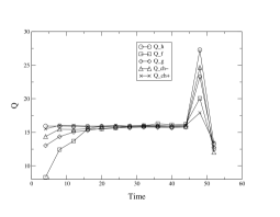
Figure 2: $Q$ factor for $L^{2}$ norms of type I data

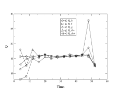
Figure 3: $Q$ factor for $L^{\infty}$ norms of type I data

3.2 Constraint Evolution

The constraint equations are not solved for in any step of our simulations, and although they are satisfied along evolution for the exact equations here we have to check this happens at the discrete level. The figures (9–9) show the $L^{\infty}$ and $L^{2}$ norm of the constraint expressions along evolution of different type of data set used. For type I data we had: $M_{Initial}=1$, $M_{Total}=1.15$, $M_{Final}=1.12$. For the type II data we introduced at the outer boundary $10$ cycles of gauge mode of frequency $2\pi$, starting at $t=10$. The black hole mass was of course constant and had the value $1$. For the type III data we introduced at the outer boundary $10$ cycles of the $\chi_{+}$ mode with frequency $2\pi$, starting at $t=10$. We had: $M_{Initial}=1$, $M_{Total}=2.6$, $M_{Final}=2.4$.

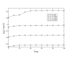
Figure 4: Log of the $L^{\infty}$ norm of $C_{f}$ of type I data

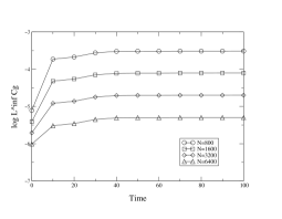
Figure 5: Log of the $L^{\infty}$ norm of $C_{g}$ of type I data

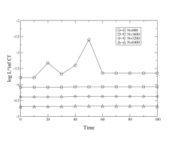
Figure 6: Log of the $L^{\infty}$ norm of $C_{f}$ of type II data

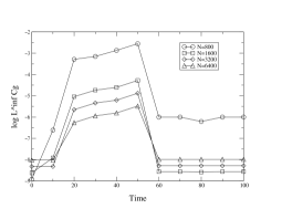
Figure 7: Log of the $L^{\infty}$ norm of $C_{g}$ of type II data

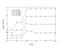
Figure 8: Log of the $L^{\infty}$ norm of $C_{f}$ of type III data

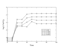
Figure 9: Log of the $L^{\infty}$ norm of $C_{g}$ of type III data

It is clear that the constraint quantities remain bounded along evolution and that they go to zero as the grid size diminishes. Most of the contribution to the $L^{\infty}$ norm comes from the boundary, where the derivative operator used is only second or third order. These peaks near de boundary can be reduced to the same level than the rest if one uses a discrete derivative operators which are fourth order at all grid points.

If one looks at the ratios $C_{f}/\frac{df}{dr}$, $C_{g}/\frac{dg}{dr}$ which in some sense measure better the failure of the constraint to be satisfied one sees that those ratios do not change so much along evolution. For $C_{f}$ the change is of only about 7%, and are of the order of $10^{-4}$. For $C_{g}$, since $g$ is chosen initially to be zero, the change at the beginning is rather big, but after a transient it gets to a plateau of the order of $10^{-4}$.

4 Results

4.1 Decay of the scalar field, ringing and power law decay

We reproduce standard results on ringing and tail (power law decay) for the first type of simulation. In figure (11) it is plotted the log of the absolute value of $\chi_{-}$ at $r=25.5$ with respect to time. It is a run where the outer boundary is at $R_{outer}=6000$, the space grid spacing was $h/M=0.0234$, where we have used the initial mass to make the ratio. footnoteIn most of the runs $k/h\approx 2$, this does not violate the Courant-Friedrichs-Lewi condition because we use Runge-Kutta for time evolution. The initial scalar field is given by a Gaussian $\chi_{+}$ pulse centered at $r=10$, giving: Initial black hole mass $M_{Initial}=1$, total mass $M_{Total}=2.56$, final black hole mass $M_{Final}=2.45$. At the beginning the characteristic ringing is seen and then a power law decay of the type $t^{\alpha}$ (this can be seen best plotting the local decay power $\displaystyle{t\frac{d\ln(\chi_{-})}{dt}}$ as defined in [4, 14], figure (11)). The power law decay computed $t^{-4.01}$ (at $t=7200$), agrees quite well from the one expected for linear perturbation theory, namely $t^{-4}$. See [12, 13]. In the plot we also show a lower resolution ($h/M=0.0468$) computation where it is clear that an instability starts to appear and become important at about half the time. This instability diminishes when the grid resolution is incremented, but still seems to be present at longer times. At the resolution used a feature departing form the power law decay is seeing after $t=7200$, this corresponds to an higher frequency mode propagating backwards at a speed $1.66$ the speed of light. These high frequency modes are common on all centered fourth order methods. Their amplitude decreases with increased precision. The time of arrival of that feature implies it originates near the inner boundary probably due to imperfect ingoing boundary conditions. After that feature, we again see (not shown in the figure) a even bigger feature, this one propagates at the correct speed of the problem, but its presence at that time implies that it is generated by the one traveling at higher speed when it enters the region near the outer boundary.

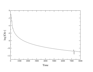
Figure 10: Decay of $\chi_{-}$ at $r=25.5$

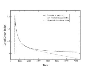
Figure 11: Power law decay of $\chi_{-}$ at $r=25.5$

The possibility of giving boundary conditions which would automatically satisfy the constraint equations allow as to perform several interesting runs. In particular we made a couple of runs of type III with

$$\chi_{+}|_{R_{out}}=A_{+}(1-\cos(\omega_{+}t))\qquad t\in[10,20]$$

with $A_{+}=1/2\pi$, and in one case $\omega=2\pi$, in the other $\omega=2\pi/10$. For these two boundary data we have,

$$\int^{20}_{10}\chi_{+}^{2}dt=15A_{+}^{2}$$

Since the energy flux is given by

$$\frac{dm}{dt}=\frac{1}{g}(\chi_{+}^{2}-\frac{(f-2)^{2}}{f^{2}}\chi_{-}^{2}),$$

and $\frac{dg}{dt}\approx\frac{2g}{fr}\chi_{+}^{2}$, $\frac{df}{dt}\approx\frac{4}{fr}\chi_{+}^{2}$, $\frac{d\chi_{-}}{dt}\approx\frac{-1}{r}\chi_{+}$. We see that to a 1% accuracy the flux of both solutions should coincide and so the black hole masses should be similar. Even more, the ringing of both solutions should be very similar, for it mostly depends on the geometry. In figure (12) we see the mass of one of the simulations and the mass difference between both simulations multiplied by 5. We see that most of the difference is bounded to the region where the wave of scalar field is moving, leaving behind the same geometry. In figure (13) we see one of the ringings (the value of $\chi_{-}$ at $r=50$) and the difference between the ringing of both solutions augmented by a factor 10. Again we see that most of the difference is at the moment where the two different wave fronts pass the point and then on the precise location of the maxima of the ringing.

Figure 12: Mass of type III run and mass difference between runs augmented 5 times.

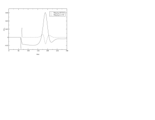
Figure 13: Values of $\chi_{-}$ at $r=50$ for a type III run, bellow the difference between runs augmented 10 times.

4.2 Relation between the initial mass and the black hole mass

We have tested the relation between the mass gap given by the total initial mass minus the final black hole mass as a function of the total initial mass for type I and type III initial-boundary data sets. In figures (15, 15) we display the results. In both cases we start with a black hole of mass unit, and put our inner boundary inside its horizon.

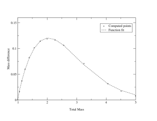
Figure 14: $\Delta M$ vs $M$ for type I data, $\Delta M=0.21*(M-1)^{0.86}\;e^{-0.55(M-1)^{1.47}}$

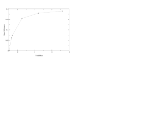
Figure 15: $\Delta M$ vs $M$ for type III data

5 Conclusions

It is difficult to see whether some of the ideas presented in this work can be extended to the full three dimensional case, where many more variables are present and where there is no preferred center in which to anchor a gauge as the one used here. But the model is so simple that perhaps the observations made in solving it can shed some light into the more difficult problem. Among the observations we have the following: a) If the gauge prescription does not fix completely the gauge it is expected there would be gauge modes propagating. In this case there was just one gauge freedom left (the value of $h$ at the initial surface and at the outer boundary), nevertheless there were three equations which acquired a non trivial propagation. b) Gauge modes, by being non-physical, can have singular behavior although the geometry given by the solution can be regular. It is clear in the model studied that the different components of the metric grow exponentially while the solution is still Schwarzschild. Thus, it seems to be necessary to isolate and keep under control the potentially unstable gauge modes. In our case this was done by choosing variables for which it was clear where the instability was, and so, choosing conveniently the initial-boundary data we could keep it small for many cases, although not always. c) The choice of gauge modes can also complicate the boundary value problem. Ideally some of the fields should acquire values at the boundary so that the constraint propagate correctly. In the model it can be seen that if part of the data for the pair $(f,g)$ must be given at the boundary (according to the values chosen for the coefficients $(K_{ff},K_{fg},K_{gg},K_{gf})$) that part must satisfy some evolution equation along the boundary, so actually there is no freedom left. But other gauge quantities, like $h$, can take any value. Thus, if the variables are not chosen appropriately it could become very cumbersome to find the correct boundary conditions which would, at the same time keep the constraint equations being satisfied and the gauge instabilities under control. Note that the procedure we used, getting some equations which are intrinsic to the boundary for some of the variables, is similar to the one used in [15], the only case where well posedness of the initial-boundary value problem in full general relativity has been asserted.

6 Acknowledgments

It is a pleasure to acknowledge several and important discussions with S. Frittelli, H.O. Kreiss, P. Laguna, and M. Tiglio.

References

- [1] Critical Phenomena in Gravitational Collapse Carsten Gundlach, Living Rev. Rel. 2:4, 1999. gr-qc/0001046
- [2] Roberto Gomez, and J. Winicour, J. Math. Phys. 33, (4), 1992.
- [3] Choptuik scaling in null coordinates, David Garfinkle, Phys. Rev. D, 51, pp.5558-5561, 1995. gr-qc/9412008
- [4] Free Evolution of nonlinear scalar field collapse in double null coordinates, Lior M. Burko, The Eighth Marcel Grossmann Meeting: Proceedings. Volume I. Edited by Tsvi Piran, Singapore, World Scientific, 1999. pp. 750-752. gr-qc/9710043
- [5] Treating instabilities in a hyperbolic formulation of Einstein’s equations, M. A. Scheel, T. W. Baumgarte, G. B. Cook, S. L. Shapiro and S. A. Teukolsky, Physical Review D, 58, 1998.
- [6] Numerical evolution of black holes with a hyperbolic formulation of general relativity, M. A. Scheel, T. W. Baumgarte, G. B. Cook, S. L. Shapiro and S. A. Teukolsky, Phys. Rev. D, 56, 1997.
- [7] Method for calculating the global structure of (singular) spacetimes, Peter Hübner, Phys. Rev. D, 53, pp. 701-721, 1996.
- [8] Conformal infinity, Living Rev. Rel., Jörg Frauendiener, http://www.livingreviews.org/Volume3/2000-4/frauendiener
- [9] Black Hole-Scalar Field Interactions in Spherical Symmetry, R. L. Marsa, and M.W. Choptuik, Phys. Rev. D, 54, 1996.
- [10] Time dependent problems and difference methods, B. Gustafsson, H.-O. Kreiss, and J. Oliger, A Wiley, 1995.
- [11] Summation by parts for finite difference approximations for d/dx, B. Strand, J. Comp. Phys., 110, 1994.
- [12] Late time behavior of stellar collapse and explosions: 1. Linearized perturbations, Carsten Gundlach, Richard H. Price, Jorge Pullin, Phys. Rev. D, 49, pp. 883-889, 1994. gr-qc/9307009
- [13] Late time behavior of stellar collapse and explosions: 2. Nonlinear evolution, Carsten Gundlach, Richard H. Price, Jorge Pullin, Phys. Rev. D, 49, pp. 890-899, 1994. gr-qc/9307010
- [14] Late time evolution of nonlinear gravitational collapse, Lior M. Burko, and Amos Ori, Phys. Rev. D 56, pp. 7820-7832, 1997. gr-qc/9703067
- [15] The initial value problem for Einstein’s vacuum field equation, H. Friedrich and G. Nagy, Commun. Math. Phys., 210, pp 619-655, 1999.