Quantum noise in second generation, signal-recycled laser interferometric gravitational-wave detectors

Abstract

It has long been thought that the sensitivity of laser interferometric gravitational-wave detectors is limited by the free-mass standard quantum limit, unless radical redesigns of the interferometers or modifications of their input/output optics are introduced. Within a fully quantum-mechanical approach we show that in a second-generation interferometer composed of arm cavities and a signal recycling cavity, e.g., the LIGO-II configuration, (i) quantum shot noise and quantum radiation-pressure-fluctuation noise are dynamically correlated, (ii) the noise curve exhibits two resonant dips, (iii) the Standard Quantum Limit can be beaten by a factor of 2, over a frequency range $\Delta f/f\!\sim\!1$, but at the price of increasing noise at lower frequencies.

PACS No.: 04.80.Nn, 95.55.Ym, 42.50.Dv, 03.65.Bz.       GRP/00/553

I Introduction

Several laser interferometric gravitational-wave (GW) detectors [1] (interferometers for short), sensitive to the high-frequency band $10-10^{3}\,{\rm Hz}$, will become operative within about one year. In the first generation of these interferometers the Laser Interferometer Gravitational Wave Observatory (LIGO), TAMA and Virgo configurations are characterized by kilometer-scale arm cavities with four mirror-endowed test masses, suspended from seismic-isolation stacks. Laser interferometry is used to monitor the relative change in the positions of the mirrors induced by the gravitational waves. The Heisenberg uncertainty principle, applied to the test masses of GW interferometers states that, if the relative positions are measured with high precision, then the test-mass momenta will be perturbed. As time passes, the momentum perturbations will produce position uncertainties, which might mask the tiny displacements produced by gravitational waves. If the momentum perturbations and measurement errors are not correlated, a detailed analysis of the above process gives rise to the standard quantum limit (SQL) for interferometers: a limiting (single-sided) noise spectral density $S_{h}^{\rm SQL}=8\hbar/(m\Omega^{2}L^{2})$ for the dimensionless gravitational-wave signal $h(t)=\Delta L/L$ [2]. Here $m$ is the mass of each identical test mass, $L$ is the length of the interferometer’s arms, $\Delta L$ is the time evolving difference in the arm lengths, $\Omega$ is the GW angular frequency, and $\hbar$ is Planck’s constant.

The concept of SQL’s for high-precision measurements was first formulated by Braginsky [3]. He also demonstrated that it is possible to circumvent SQL’s by changing the designs of the instruments, so they measure quantities which are not affected by the uncertainty principle by virtue of commuting with themselves at different times [3], [4] – as for example in speed-meter interferometers [5], which measure test-mass momenta instead of positions. Interferometers that circumvent the SQL are called quantum-nondemolition (QND) interferometers. Since the early 1970s, it has been thought that to beat the SQL for GW interferometers the redesign must be major. Examples are (i) speed-meter designs [5] with their radically modified optical topology, (ii) the proposal to inject squeezed vacuum into an interferometer’s dark port [6], and (iii) the proposal to introduce two kilometer-scale filter cavities into the interferometer’s output port [7] so as to implement frequency-dependent homodyne detection [8]. Both (ii) and (iii) intend to take advantage of the non-classical correlations of the optical fields. These radical redesigns require high laser power circulating in the arm cavities ($\raise 1.72218pt\hbox{$>$}\kern-6.99997pt\lower 2.6694pt\hbox{$\sim$}\,1$ MW) and/or are strongly susceptible to optical losses which tend to destroy quantum correlations. In order to tackle these two important issues, Braginsky, Khalili and colleagues have recently proposed the GW “optical bar” scheme [9], where the test mass is effectively an oscillator, whose restoring force is provided by in-cavity optical fields. For “optical bar” detectors the free-mass SQL is no more relevant and one can beat the SQL using classical techniques of position monitoring. Moreover, this scheme has two major advantages: It requires much lower laser power circulating in the cavities [9], and is less susceptible to optical losses.

Research has also been carried out using successive independent monitors of free-mass positions. Yuen, Caves and Ozawa discussed and disputed about the applicability and the beating of the SQL within such models [10]. Specifically, Yuen and Ozawa conceived ways to beat the SQL by taking advantage of the so-called contractive states [10]. However, the class of interaction Hamiltonians given by Ozawa are not likely to be applicable to GW interferometers (for further details see Ref. [11]).

Recently, we showed [12] that it is possible to circumvent the SQL for LIGO-II-type signal-recycling (SR) interferometers [13, 14]. With their currently planned design, LIGO-II interferometers can beat the SQL by modest amounts, roughly a factor two over a bandwidth $\Delta f\!\sim\!f$. It is quite interesting to notice that the beating of the SQL in SR interferometers has a similar origin as in “optical bar” GW detectors mentioned above [9].

Braginsky and colleagues [16], building on earlier work of Braginsky and Khalili [4], have shown that for LIGO-type GW interferometers, the test-mass initial quantum state only affects frequencies $\,\raise 1.72218pt\hbox{$<$}\kern-8.00003pt\lower 2.6694pt\hbox{$\sim$}\,1$ Hz, the dependence on the initial quantum state can be removed filtering the output data at low frequency. Therefore, the SQL in GW interferometers is enforced only by the light’s quantum noise, not directly by the test mass. As we discussed in [12], and we shall explicitly show below, we can decompose the optical noise of a SR interferometer into shot noise and radiation-pressure noise, using the fact that they transform differently under rescaling of the mirror mass $m$ and the light power $I_{o}$. As long as there are no correlations between the light’s shot noise and its radiation-pressure-fluctuation noise, the light firmly enforces the SQL. This is the case for conventional interferometers, i.e. for interferometers that have no SR mirror at the output dark port and a simple homodyne detection is performed (the type of interferometer used in LIGO-I/TAMA/Virgo). However, the SR mirror [13, 14] (which is being planned for LIGO-II  as a tool to reshape the noise curve, and thereby improve the sensitivity to specific GW sources [17] ) produces dynamical shot-noise / back-action-noise correlations, and these correlations break the light’s ability to enforce the SQL. These dynamical correlations come naturally from the nontrivial coupling between the test mass and the signal-recycled optical fields, which makes the dynamical properties of the entire optical-mechanical system rather different from the naive picture of a free mass buffeted by Poissonian radiation pressure. As a result, the SQL for a free test mass has no relevance for a SR interferometer. Its only remaining role is as a reminder of the regime where back-action noise is comparable to the shot noise. The remainder of this paper is devoted to explaining these claims in great detail. To facilitate the reading we have put our discussion of the dynamical system formed by the optical fields and the mirrors into a separate, companion paper [11].

The outline of this paper is as follows. In Sec. II we derive the input–output relations for the whole optical system composed of arm cavities and a SR cavity, pointing out the existence of dynamical instabilities, and briefly commenting on the possibility and consequences of introducing a control system to suppress them. In Sec. III we evaluate the spectral density of the quantum noise. More specifically, in Sec. III A we discuss the general case, showing that LIGO-II can beat the SQL when dynamical correlations between shot noise and radiation-pressure noise are produced by the SR mirror. In Sec. III B, making links to previous investigations, we decompose our expression for the optical noise into shot noise and radiation-pressure noise and express the dynamical correlations between the two noises in terms of physical parameters characterizing the SR interferometer; in Sec. III C we specialize to two cases, the extreme signal-recycling (ESR) and extreme resonant-sideband-extraction (ERSE) configurations, where dynamical correlations are absent and a semiclassical approach can be applied [13, 14]. In Sec. IV we investigate the structure of resonances of the optical-mechanical system and discuss their link to the minima present in the noise curves. Finally, Sec. V deals with the effects of optical losses, while Sec. VI summarizes our main conclusions. The Appendix discusses the validity of the two-photon formalism in our context.

II Signal-recycling interferometer: input–output relations

In Fig. 1 we sketch the SR configuration of LIGO-II interferometers. The optical topology inside the dashed box is that of conventional interferometers such as LIGO-I/TAMA/Virgo, which are Michelson interferometers with Fabry-Perot (FP) arm cavities. The principal noise input and the signal and noise output for the conventional topology are $c_{i}$ and $d_{i}$ in Fig. 1. In a recent paper, KLMTV [7] have derived the input–output $(c_{i}-d_{i})$ relations for a conventional interferometer at the output dark port, immediately after the beam splitter, within a full quantum mechanical approach. In this section we shall derive the input–output $(a_{i}-b_{i})$ relations for the whole optical system at the output port, i.e. immediately after the SR mirror, and shall evaluate the corresponding noise spectral density.

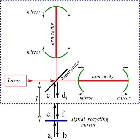
FIG. 1.: Schematic view of a LIGO-II signal-recycling interferometer. The interior of the dashed box refers to the conventional interferometer; $c_{i}$ and $d_{i}$ are the input and output fields at the beam splitter’s dark port; $a_{i}$ and $b_{i}$ are the vacuum input and signal output of the whole optical system. The laser light enters the bright port of the beam splitter. The arrows close to arm cavities’ extremities indicate gravitational-wave-induced mirror displacements.

As we shall see, a naive application of the Fourier-based formalism developed in [7] gives ill-defined input–output relations, due to the presence of optical-mechanical instabilities. These instabilities have an origin similar to the dynamical instability of a detuned FP cavity induced by the radiation-pressure force acting on the mirrors, which has long been investigated in the literature [18, 19, 20]. To suppress the growing modes and make the KLMTV’s formalism valid for SR interferometers, an appropriate control system should be introduced. The analysis of the resulting interferometer plus controller requires a detailed description of the dynamics of the whole system and for this we have found Braginsky and Khalili’s theory of linear quantum measurement [4] very powerful and intuitive. We analyzed the details of the dynamics in an accompanying paper [11], showing in particular that the results derived in this section by Fourier techniques, notably the noise spectral density curves, are correct and rigorously justified.

A Naive extension of KLMTV’s results to SR interferometers

As in Ref. [7] we shall describe the interferometer’s light by the electric field evaluated on the optic axis (center of light beam) and at specific, fixed locations along the optic axis. Correspondingly, the electric fields that we write down will be functions of time only: all dependence on spatial position will be suppressed from our formulae.

Quantity	Symbol & value for LIGO-II	Quantity	Symbol & value for LIGO-II
Light power at beam splitter	$I_{o}$	Light power to reach SQL	$I_{\rm SQL}=1.0\times 10^{4}$ W
SQL for GW detection	$h^{2}_{\rm SQL}\equiv S_{h}^{\rm SQL}=4\times 10^{-48}/{\rm Hz}$	Arm-cavity half bandwidth	$\gamma=Tc/4L=2\pi\times 100\,{\rm sec}^{-1}$
Laser angular frequency	$\omega_{o}=1.8\times 10^{15}\,{\rm sec}^{-1}$	GW angular frequency	$\Omega$
End-mirror mass	$m=30$ kg	Arm-cavity length	$L=4$ km
SR cavity length	$l\approx 10$ m	Internal arm-cavity mirror transmissivity	$T=0.033$ (power)
SR mirror transmissivity	$\tau$ (amplitude)	SR cavity detuning	$\phi$
Arm-cavity power loss	$\epsilon=0.01$	SR power loss	$\lambda_{\rm SR}=0.02$
Photodetector loss	$\lambda_{\rm PD}=0.1$

TABLE I.: Summary of LIGO-II parameters [21].

The input field at the bright port of the beam splitter, which is assumed to be infinitesimally thin, is a carrier field, described by a coherent state with power $I_{o}$ and angular frequency $\omega_{o}$. We assume [7] that the arm-cavity end mirrors oscillate around an equilibrium position that is on resonance with the carrier light. This means that there is no zeroth-order arm-cavity detuning (see the paper of Pai et al. [20] for a critical discussion of this assumption). Our most used interferometer parameters are given in Table I together with the values anticipated for LIGO-II.

We denote by $f_{\rm GW}=\Omega/2\pi$ the GW frequency, which lies in the range $10-1000$ Hz. Then the interaction of a gravitational wave with the optical system produces side-band frequencies $\omega_{o}\pm\Omega$ in the electromagnetic field at the output dark port. For this reason, similarly to KLMTV [7], we find it convenient to describe the quantum optics inside the interferometer using the two-photon formalism developed by Caves and Schumaker [22, 23]. In this formalism, instead of using the usual annihilation and creation operators for photons at frequency $\omega$, we expand the field operators in terms of quadrature operators which can simultaneously annihilate a photon at frequency $\omega=\omega_{o}+\Omega$ while creating a photon at frequency $\omega=\omega_{o}-\Omega$ (or vice versa).

More specifically, the quantized electromagnetic field in the Heisenberg picture evaluated at some fixed point on the optic axis, and restricted to the component propagating in one of the two directions along the axis is:

$$\widehat{E}(t)=\sqrt{\frac{2\pi\hbar}{{\cal A}\,c}}\,\int_{0}^{+\infty}\sqrt{\omega}\,\left[\widehat{a}_{\omega}\,e^{-i\omega t}+\widehat{a}^{\dagger}_{\omega}\,e^{+i\omega t}\right]\,\frac{d\omega}{2\pi}\,.$$ (1)

Here ${\cal A}$ is the effective cross sectional area of the laser beam and $c$ is the speed of light. The annihilation and creation operators $\widehat{a}_{\omega}$, $\widehat{a}_{\omega}^{\dagger}$ in Eq. (1), which in the Heisenberg picture are fixed in time, satisfy the usual commutation relations

$$[\widehat{a}_{\omega},\widehat{a}_{\omega^{\prime}}]=0\,,\quad\quad[\widehat{a}^{\dagger}_{\omega},\widehat{a}^{\dagger}_{\omega^{\prime}}]=0\,,\quad\quad[\widehat{a}_{\omega},\widehat{a}_{\omega^{\prime}}^{\dagger}]=2\pi\,\delta(\omega-\omega^{\prime})\,.$$ (2)

Henceforth, to ease the notation we shall omit the hats on quantum operators. Defining the new operators (see Sec. IV of Ref. [22] )

$$a_{+}\equiv a_{\omega_{o}+\Omega}\,\sqrt{\frac{\omega_{o}+\Omega}{\omega_{o}}}\,,\quad\quad a_{-}\equiv a_{\omega_{o}-\Omega}\,\sqrt{\frac{\omega_{o}-\Omega}{\omega_{o}}}\,,$$ (3)

and using the commutation relations (2), we find

$$[a_{+},a_{+^{\prime}}^{\dagger}]=2\pi\,\delta(\Omega-\Omega^{\prime})\,\left(1+\frac{\Omega}{\omega_{o}}\right)\,,\quad\quad[a_{-},a_{-^{\prime}}^{\dagger}]=2\pi\,\delta(\Omega-\Omega^{\prime})\,\left(1-\frac{\Omega}{\omega_{o}}\right)\,,$$ (4)

$$[a_{+},a_{+^{\prime}}]=0=[a_{-},a_{-^{\prime}}]\,,\quad\quad[a_{+}^{\dagger},a_{+^{\prime}}^{\dagger}]=0=[a_{-}^{\dagger},a_{-^{\prime}}^{\dagger}]\,,\quad\quad[a_{+},a_{-^{\prime}}]=0=[a_{+},a_{-^{\prime}}^{\dagger}]\,,$$ (5)

where $a_{\pm^{\prime}}$ stands for $a_{\pm}(\Omega^{\prime})$. Because the carrier frequency is $\omega_{o}\simeq 10^{15}\,\rm s^{-1}$ and we are interested in frequencies $\Omega/2\pi$ in the range $10\,--\,10^{3}$ Hz, we shall disregard in Eq. (5) the term proportional to $\Omega/\omega_{o}$. (In the Appendix we shall give a more complete justification of this by evaluating the effect the term proportional to $\Omega/\omega_{o}$ would have on the final noise spectral density.) We can then rewrite the electric field, Eq. (1), as

$$E(t)=\sqrt{\frac{2\pi\hbar\,\omega_{o}}{{\cal A}\,c}}\,e^{-i\omega_{o}\,t}\,\int_{0}^{+\infty}(a_{+}(\Omega)\,e^{-i\Omega t}+a_{-}(\Omega)\,e^{i\Omega t})\,\frac{d\Omega}{2\pi}+{\rm h.c.}\,,$$ (6)

where “h.c.” means Hermitian conjugate. Following the Caves-Schumaker two-photon formalism [22, 23], we introduce the amplitudes of the two-photon modes as

$$a_{1}=\frac{a_{+}+a_{-}^{\dagger}}{\sqrt{2}}\,,\quad\quad a_{2}=\frac{a_{+}-a_{-}^{\dagger}}{\sqrt{2}i}\,;$$ (7)

$a_{1}$ and $a_{2}$ are called quadrature fields and they satisfy the commutation relations

$$[a_{1},a_{2^{\prime}}^{\dagger}]=-[a_{2},a_{1^{\prime}}^{\dagger}]=2\pi i\delta(\Omega-\Omega^{\prime})\,,$$ (8)

$$[a_{1},a_{1^{\prime}}^{\dagger}]=0=[a_{1},a_{1^{\prime}}]\,,\quad\quad[a_{2},a_{2^{\prime}}^{\dagger}]=0=[a_{2},a_{2^{\prime}}]\,.$$ (9)

Expressing the electric field (6) in terms of the quadratures we finally get

$$E(a_{i};t)=\cos(\omega_{o}\,t)\,E_{1}(a_{1};t)+\sin(\omega_{o}\,t)\,E_{2}(a_{2};t)\,,$$ (10)

with

$$E_{j}(a_{j};t)=\sqrt{\frac{4\pi\hbar\,\omega_{o}}{{\cal A}\,c}}\,\int_{0}^{+\infty}(a_{j}\,e^{-i\Omega t}+a_{j}^{\dagger}\,e^{i\Omega t})\,\frac{d\Omega}{2\pi}\quad\quad j=1,2\,.$$ (11)

Note (as is discussed at length by BGKMTV [16] and was previewed by KLMTV (footnote 1 of Ref. [7])), that, $E_{1}(t)$ and $E_{2}(t)$ commute with themselves at any two times $t$ and $t^{\prime}$, i.e. $[E_{j}(t),E_{j}(t^{\prime})]=0$, while $[E_{1}(t),E_{2}(t^{\prime})]\!\sim\!i\delta(t-t^{\prime})$. Hence, the quadrature fields $E_{j}(t)$ with $j=1,2$ are quantum-nondemolition quantities which can be measured with indefinite accuracy over time, i.e. measurements made at different times can be stored as independent bits of data in a classical storage medium without being affected by mutually-induced noise, while it is not possible to do this for $E_{1}(t)$ and $E_{2}(t)$ simultaneously. As BGKMTV [16] emphasized (following earlier work by Braginsky and Khalili [4]), this means that we can regard $E_{1}(t)$ and $E_{2}(t)$ separately as classical variables – though in each other’s presence they behave nonclassically.

For GW interferometers the full input electric field at the dark port is $E(c_{i};t)$ where $c_{1}$ and $c_{2}$ are the two input quadratures, while the output field at the dark port is $E(d_{i};t)$, with $d_{1}$ and $d_{2}$ the two output quadratures (see Fig. 1). Assuming that the classical laser-light input field at the beam splitter’s bright port is contained only in the first quadrature, and evaluating the back-action force acting on the arm-cavity mirrors disregarding the motion of the mirrors during the light round-trip time (quasi-static approximation), KLMTV [7] derived the following input–output relations at side-band (GW) angular frequency $\Omega$

$$d_{1}=c_{1}\,e^{2i\beta}\,,\quad\quad d_{2}=(c_{2}-{\cal K}c_{1})\,e^{2i\beta}+\sqrt{2{\cal K}}\,\frac{h}{h_{\rm SQL}}\,e^{i\beta}\,,$$ (12)

where $2\beta=2\arctan{{\Omega}/{\gamma}}$ is the net phase gained by the sideband frequency $\Omega$ while in the arm-cavity, $\gamma=Tc/4L$ is the half bandwidth of the arm-cavity ($T$ is the power transmissivity of the arm-cavity input mirrors and $L$ is the length of the arm cavity), $h$ is the Fourier transform of the gravitational-wave field, and $h_{\rm SQL}$ is the SQL for GW detection, explicitly given by

$$h_{\rm SQL}(\Omega)\equiv\sqrt{S_{h}^{\rm SQL}}=\sqrt{\frac{8\hbar}{m\Omega^{2}L^{2}}}\,,$$ (13)

where $m$ is the mass of each arm-cavity mirror. The quantity ${\cal K}$ in Eq. (12) is the effective coupling constant, which relates the motion of the test mass to the output signal,

$${\cal K}=\frac{2(I_{o}/I_{\rm SQL})\gamma^{4}}{\Omega^{2}(\gamma^{2}+\Omega^{2})}\,.$$ (14)

Finally, $I_{o}$ is the input light power, and $I_{\rm SQL}$ is the light power needed by a conventional interferometer to reach the SQL at a side band frequency $\Omega=\gamma$, that is

$$I_{\rm SQL}=\frac{m\,L^{2}\,\gamma^{4}}{4\omega_{o}}\,.$$ (15)

(See in Table I the values of the interferometer parameters tentatively planned for LIGO-II [21].) We shall now derive the new input–output $(a_{i}-b_{i})$ relations including the SR cavity. We indicate by $l$ the length of the SR cavity and we introduce two dimensionless variables: $\phi\equiv[\omega_{o}l/c]_{{\rm mod}\,2\pi}$, the phase gained by the carrier frequency $\omega_{o}$ while traveling one way in the SR cavity, and $\Phi\equiv[\Omega l/c]_{{\rm mod}\,2\pi}$ the additional phase gained by the sideband with GW frequency $\Omega$ (see Fig. 1). Note that we are assuming that the distances from the beam splitter to the two arm-cavity input mirrors are identical, equal to an integer multiple of the carrier light’s wavelength, and are negligible compared to $l$.

Propagating the output electric field $E(d_{i};t)$ up to the SR mirror, and introducing the operators $e_{i}$ and $f_{i}$ which describe the fields that are immediately inside the SR mirror (see Fig. 1), we get the condition

$$E(f_{i};t)=E\left(d_{i};t-\frac{l}{c}\right)\,,$$ (16)

which, together with Eq. (10), provides the following equations

$$f_{1}=(d_{1}\,\cos{\phi}-d_{2}\,\sin{\phi})\,e^{i\Phi}\,,\quad\quad f_{2}=(d_{1}\,\sin{\phi}+d_{2}\,\cos{\phi})\,e^{i\Phi}\,.$$ (17)

Proceeding in an analogous way for the input electric field $E(c_{i};t)$, we derive

$$e_{1}=(c_{1}\,\cos{\phi}+c_{2}\,\sin{\phi})\,e^{-i\Phi}\,,\quad\quad e_{2}=(-c_{1}\,\sin{\phi}+c_{2}\,\cos{\phi})e^{-i\Phi}\,.$$ (18)

Note that each of Eqs. (17), (18) correspond to a rotation of the quadratures $d_{1}$, $d_{2}$ (or $c_{1}$, $c_{2}$) plus the addition of an overall phase. Finally, denoting by $a_{i}$ and $b_{i}$ the input and output fields of the whole system at the output port (see Fig. 1) we conclude that the following relations should be satisfied at the SR mirror:

$$e_{1}=\tau\,a_{1}+\rho\,f_{1}\,,\quad\quad e_{2}=\tau\,a_{2}+\rho\,f_{2}\,,$$ (19)

$$b_{1}=\tau\,f_{1}-\rho\,a_{1}\,,\quad\quad\,\,b_{2}=\tau\,f_{2}-\rho\,a_{2}\,,$$ (20)

where $\pm\rho$ and $\tau$ are the amplitude reflectivity and transmissivity of the SR mirror, respectively. We use the convention that $\rho$ and $\tau$ are real and positive, with the reflection coefficient being $+\rho$ for light coming from inside the cavity and $-\rho$ for light coming from outside. In this section we limit ourselves to a lossless SR mirror; therefore the following relation holds: $\tau^{2}+\rho^{2}=1$.

Before giving the solution of the above equations, let us notice that the equations we derived so far for the quantum EM fields in the Heisenberg picture are exactly the same as those of classical EM fields. To deduced them it is sufficient to replace the quadrature operators by the Fourier components of the classical EM fields. The input-output relation we shall give below is also the same as in the classical case. In the latter we should assume that a fluctuating field enters the input port of the entire interferometer. More specifically, assuming a vacuum state in the input port, we can model the two input quadrature fields as two independent white noises. Then using the classical equations, we can derive the output fields which have the correct noise spectral densities.

Solving the system of Eqs. (12), (17)–(20) gives the final input–output relation:

$$\left(\matrix{b_{1}\cr b_{2}}\right)=\frac{1}{M}\left[e^{2i(\beta+\Phi)}\left(\matrix{C_{11}&C_{12}\cr C_{21}&C_{22}}\right)\left(\matrix{a_{1}\cr a_{2}}\right)+\sqrt{2{\cal K}}\tau e^{i(\beta+\Phi)}\left(\matrix{D_{1}\cr D_{2}}\right)\frac{h}{h_{\rm SQL}}\right]\,,$$ (21)

where, to ease the notation, we have defined:

$$M=1+\rho^{2}\,e^{4i(\beta+\Phi)}-2\rho\,e^{2i(\beta+\Phi)}\left(\cos{2\phi}+\frac{{\cal K}}{2}\,\sin{2\phi}\right)\,,$$ (22)

$$C_{11}=C_{22}=(1+\rho^{2})\,\left(\cos{2\phi}+\frac{{\cal K}}{2}\,\sin{2\phi}\right)-2\rho\,\cos{(2(\beta+\Phi))}\,,$$ (23)

$$C_{12}=-\tau^{2}\,(\sin{2\phi}+{\cal K}\,\sin^{2}{\phi})\,,\quad\quad C_{21}=\tau^{2}\,(\sin{2\phi}-{\cal K}\,\cos^{2}{\phi})\,,$$ (24)

$$D_{1}=-(1+\rho\,e^{2i(\beta+\Phi)})\,\sin{\phi}\,,\quad\quad D_{2}=-(-1+\rho\,e^{2i(\beta+\Phi)})\,\cos{\phi}\,.$$ (25)

A straightforward calculation using $C_{ij}\in\Re$ and $C_{11}\,C_{22}-C_{12}\,C_{21}=|M|^{2}$, confirms that the quadratures $b_{i},b_{i}^{\dagger}$ satisfy the commutation relations (8), as they should since like $a_{i}$ and $a_{i}^{\dagger}$ they represent free fields. Let us also observe that both the quadratures $b_{1}$ and $b_{2}$ in Eq. (21) contain the gravitational-wave signal $h$ and that it is not possible to put the signal into just one of the quadratures through a transformation that preserves the commutation relations of $b_{1}$ and $b_{2}$. Indeed, the most general transformation that preserves the commutation relations is of the form

$$\left(\matrix{\widetilde{b}_{1}\cr\widetilde{b}_{2}}\right)=e^{i\,\alpha}\,\left(\matrix{L_{11}&L_{12}\cr L_{21}&L_{22}}\right)\left(\matrix{b_{1}\cr b_{2}}\right)\,,\quad\quad L_{ij}\in\Re\,,\quad\det{L_{ij}}=1\,,$$ (26)

where $\alpha$ is an arbitrary phase. Because the $D_{i}$ are complex [see Eq. (25)], it is impossible to null the $h$ contribution either in $\widetilde{b}_{1}$ or $\widetilde{b}_{2}$.

Henceforth, we limit our analysis to $\Phi=0$, which corresponds to a SR cavity much shorter than the arm-cavities, e.g., $l\simeq 10\,{\rm m}$. We assume for simplicity that there is no radio-frequency (MHz) modulation/demodulation of the carrier and the signal [21]; instead, some frequency-independent quadrature

$$b_{\zeta} =b_{1}\,\sin\zeta+b_{2}\,\cos\zeta$$ (29)

$$=\frac{1}{M}\,\left[e^{2i\beta}(C_{11}\,\sin\zeta+C_{21}\,\cos\zeta)\,a_{1}+e^{2i\beta}(C_{12}\,\sin\zeta+C_{22}\,\cos\zeta)\,a_{2}\right.$$

$$\left.+\sqrt{2{\cal K}}\,\tau\,e^{i\beta}\,(D_{1}\,\sin\zeta+D_{2}\,\cos\zeta)\,\frac{h}{h_{\rm SQL}}\right]\,,$$

is measured via homodyne detection [8]. Before going on to evaluate the noise spectral density in the measured quadrature $b_{\zeta}$, let us first comment on the results obtained in this section.

B Discussion of the naive result

There is a major delicacy in the input–output relation given by Eq. (19). By naively transforming it from the frequency domain back into the time domain, we deduce that the output quadratures depend on the gravitational-wave field and the input optical fields both in the past and in the future. Mathematically this is due to the fact that the coefficient $1/M$, in front of $h$ and $a_{i}$ ($i=1,2$) in Eq. (21), contains poles both in the lower and in the upper complex plane. This situation is a very common one in physics and engineering (it occurs for example in the theory of linear electronic networks [25] and the theory of plasma waves [26]), and the cure for it is well known: in order to construct an output field that only depends on the past, we have to alter the integration contour in the inverse-Fourier transform, going above (with our convention of Fourier transform) all the poles in the complex plane. This procedure, which can be justified rigorously using Laplace transforms [27], makes the output signal infinitely sensitive to driving forces in the infinitely distant past. The reason is simple and well known in other contexts: our optical mechanical system possesses instabilities, which can be deduced from the homogeneous solution $b_{i}^{\rm hom}$ of Eqs. (12), (16) and (20), which has eigenfrequencies given by $M=0$. Because the zeros of the equation $M=0$ are generically complex and may have positive imaginary parts [11], we end up with homogeneous solutions that grow exponentially.

To quench the instabilities of a SR interferometer we have to introduce a proper control system. In [11] we have given an example of such a control system, which we briefly illustrate here. Let us suppose that the observed output is $b_{\zeta}$ and we feed back a linear transformation of it to control the dynamics of the end mirrors. This operation corresponds to making the following substitution in Eq. (29):

$$h\rightarrow h+{\cal C}\,b_{\zeta},$$ (30)

where ${\cal C}$ is some retarded kernel. Solving again for $b_{\zeta}$, we get:

$$b_{\zeta}^{\cal C} =\frac{1}{{M}_{\cal C}}\,\left[e^{2i\beta}(C_{11}\,\sin\zeta+C_{21}\,\cos\zeta)\,a_{1}+e^{2i\beta}(C_{12}\,\sin\zeta+C_{22}\,\cos\zeta)\,a_{2}\right.$$ (32)

$$\left.+\sqrt{2{\cal K}}\,\tau\,e^{i\beta}\,(D_{1}\,\sin\zeta+D_{2}\,\cos\zeta)\,\frac{h}{h_{\rm SQL}}\right]\,,$$

simply replacing the $M$ in (29) by $M_{\cal C}$, which depends on $\cal C$. Note that, by contrast with the uncontrolled output Eq. (21), the output field $b_{\zeta}^{\cal C}$ is no longer a free electric field, i.e. a quadrature field defined in half open space, satisfying the radiative boundary condition. This is due to the fact that part of it has been fed back into the arm cavities. Nevertheless, in the time domain, $b_{\zeta}^{\cal C}$ commutes with itself at different times. In [11] we have shown that there exists a well-defined $\cal C$ that makes Eq. (32) well defined in the time domain, getting rid of the instabilities. As a consequence, $M_{\cal C}$ has zeros only in the lower-half complex plane and we can neglect the homogeneous solution $M_{\cal C}\,b_{\zeta}^{{\cal C}\,\rm hom}=0$ because it decays exponentially in time.

Finally, let us remember the important fact that the introduction of this kind of control system only changes the normalization of the output field. As a consequence, the noise spectral density is not affected. However, an extra noise will be present due to the electronic device that provides the control force on the end mirrors. K. Strain estimated that it can be kept smaller than about $10\%$ of the quantum noise [28].

III Features of noise spectral density in SR interferometers

In light of the discussion at the end of the last section, we shall use Eq. (32) as the starting point of our derivation of the noise spectral density of a (stabilized) SR interferometer.

A Evaluation of the noise spectral density: going below the standard quantum limit

The noise spectral density is calculated as follows [7]. Equation (32) tells us that the interferometer noise, expressed as an equivalent gravitational-wave Fourier component, is

$$h_{n}\equiv\frac{h_{\rm SQL}}{\sqrt{2{\cal K}}}\,\Delta b_{\zeta}\,,$$ (33)

where

$$\Delta b_{\zeta}=\frac{(C_{11}\,\sin\zeta+C_{21}\,\cos\zeta)\,a_{1}+(C_{12}\,\sin\zeta+C_{22}\,\cos\zeta)\,a_{2}}{\tau\,(D_{1}\,\sin\zeta+D_{2}\,\cos\zeta)}\,.$$ (34)

Then the (single-sided) spectral density $S^{\zeta}_{h}(f)$, with $f=\Omega/2\pi$, associated with the noise $h_{n}$ can be computed by the formula (Eq. (22) of Ref. [7])

$$\frac{1}{2}\,2\pi\,\delta(\Omega-\Omega^{\prime})\,S^{\zeta}_{h}(f)=\langle{\rm in}|h_{n}(\Omega)\,h_{n}^{\dagger}(\Omega^{\prime})|{\rm in}\rangle_{\rm sym}\equiv\frac{1}{2}\langle{\rm in}|h_{n}(\Omega)\,h_{n}^{\dagger}(\Omega^{\prime})+h_{n}^{\dagger}(\Omega^{\prime})\,h_{n}(\Omega)|{\rm in}\rangle\,.$$ (35)

Here we put the superscript $\zeta$ on $S^{\zeta}_{h}$ to remind ourselves that this is the noise when the output is monitored at carrier phase $\zeta$ by homodyne detection. Assuming that the input of the whole SR interferometer is in its vacuum state, as is planned for LIGO-II, i.e. $|{\rm in}\rangle=|0_{a}\rangle$, and using

$$\langle 0_{a}|a_{i}\,a^{\dagger}_{j^{\prime}}|0_{a}\rangle_{\rm sym}=\frac{1}{2}\,2\pi\,\delta(\Omega-\Omega^{\prime})\,\delta_{ij}\,,$$ (36)

(Eq. (25) of Ref. [7]) we find that Eq. (35) can be recast in the simple form (note that $C_{ij}\in\Re$):

$$S_{h}^{\zeta}=\frac{h_{\rm SQL}^{2}}{2{\cal K}}\,\frac{\left(C_{11}\,\sin\zeta+C_{21}\,\cos\zeta\right)^{2}+\left(C_{12}\,\sin\zeta+C_{22}\,\cos\zeta\right)^{2}}{\tau^{2}\,\left|D_{1}\,\sin\zeta+D_{2}\,\cos\zeta\right|^{2}}\,.$$ (37)

For comparison, let us recall some properties of the noise spectral density for conventional interferometers (for a complete discussion see Ref. [7]). To recover this case we have to take the limit $\phi\rightarrow 0$ and $\rho\rightarrow 0$ in the above equations or simply use Eq. (12) (in a conventional interferometer there are no instabilities). In particular, for a conventional interferometer, Eqs. (29) and (33) take the much simpler form

$$b^{\rm conv}_{\zeta}=\cos\zeta\,\{\left[a_{2}+(\tan\zeta-{\cal K})\,a_{1}\right]\,e^{2i\beta}\}\,,\quad\quad h_{n}^{\rm conv}=\frac{h_{\rm SQL}}{\sqrt{\cal K}}\,e^{i\beta}\,\left[a_{2}+(\tan\zeta-{\cal K})\,a_{1}\right]\,,$$ (38)

and the noise spectral density reads

$$S_{h}^{\zeta,\rm conv}=\frac{h_{\rm SQL}^{2}}{2{\cal K}}\,\left[1+(\tan\zeta-{\cal K})^{2}\right]\,.$$ (39)

As has been much discussed by Matsko, Vyatchanin and Zubova [8] and by KLMTV [7], and as we shall see in more detail in Sec. III B, taking as the output $b_{\zeta}$, instead of the quadrature $b_{2}$ in which all the signal $h$ is encoded, builds up correlations between shot noise and radiation-pressure noise. We refer to correlations of this kind, which are introduced by the special read-out scheme, as static correlations by contrast with those produced by the SR mirror, which we call dynamical since they are built up dynamically, as we shall discuss in Sec. IV. The static correlations allow the noise curves for a conventional interferometer to go below the SQL when $I_{o}=I_{\rm SQL}$, as was originally observed by Matsko, Vyatchanin and Zubova [8]. However, if $\zeta$ is frequency independent as it must be when one uses conventional homodyne detection, then the SQL is beaten, $S_{h}^{\zeta,\rm conv}\leq h^{2}_{\rm SQL}$, only over a rather narrow frequency band and only by a very modest amount. On the other hand, as Matsko, Vyatchanin and Zubova [8] showed, and one can see from Eq. (39), if we could make the homodyne detection angle $\zeta$ frequency dependent, then choosing [7] $\zeta(\Omega)\equiv\arctan{\cal K}(\Omega)$, would remove completely (in the absence of optical losses) the second term in the square parenthesis of Eq. (39), which is the radiation-pressure noise, leaving only the shot noise in the interferometer output, i.e. $S_{h}^{\zeta,\rm conv}={h_{\rm SQL}^{2}}/{2{\cal K}}$. In order to implement frequency dependent homodyne detection, KLMTV [7] have recently propose to place two 4km-long filter cavities at the interferometer dark port and follow them by conventional homodyne detection. This experimentally challenging proposal would allow the interferometer to beat the SQL at frequency $f=100$ Hz by a factor $\sqrt{S_{h}^{\rm conv}}/\sqrt{S_{h}^{\rm SQL}}\!\sim\!0.24$, over a band of $\Delta f\!\sim\!f$, at light power $I_{o}=I_{\rm SQL}$, and by $\sqrt{S_{h}^{\rm conv}}/\sqrt{S_{h}^{\rm SQL}}\!\sim\!0.18$ if $I_{o}\simeq 3.2I_{\rm SQL}$. In conclusion, already in conventional interferometers it is possible to beat the SQL provided that we measure $b_{\zeta}$ and build up proper static correlations between shot noise and radiation-pressure noise.

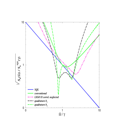
FIG. 2.: Log-log plot of $\sqrt{S_{h}(\Omega)}/\sqrt{S_{h}^{\rm SQL}(\gamma)}$ versus $\Omega/\gamma$ for (i) the quadratures $b_{1}^{\cal C}$ ($\zeta=\pi/2$) and $b_{2}^{\cal C}$ ($\zeta=0$) with $\rho=0.9$, $\phi=\pi/2-0.47$ and $I_{o}=I_{\rm SQL}$, (ii) the SQL, (iii) a conventional interferometer with $I_{o}=I_{\rm SQL}$, and (iv) the noise curve of LIGO-II [21] one would obtain if shot-noise / radiation-pressure correlations were (naively) neglected. For LIGO-II, $\gamma=2\pi\times 100\,{\rm Hz}$ (top axis) and $\sqrt{S_{h}^{\rm SQL}(\gamma)}=2\times 10^{-24}\,{\rm Hz}^{-1/2}$. These curves do not include seismic and thermal noises; for LIGO-II the latter is expected to be slightly above the SQL [15].

Let us now go back to SR interferometers. They have the interesting property of building up dynamically the correlations between shot noise and radiation-pressure noise, thanks to the SR mirror. Indeed, even if we restrict ourselves to the noise curves associated with the two quadratures $b_{1}^{\cal C}$ and $b_{2}^{\cal C}$, i.e. we do not measure $b_{\zeta}^{\cal C}$, the SR interferometer can still go below the SQL. Moreover, if the SR interferometer works at the SQL power, i.e. $I_{o}=I_{\rm SQL}$, as is tentatively planned for LIGO-II, then the noise curves [Eq. (37)] can exhibit one or two resonant dips whose depths increase and widths decrease as the SR-mirror’s reflectivity is raised. (We postpone the discussion of this interesting feature to Sec. IV.) These resonances allow us to reshape the noise curves and beat the SQL by much larger amounts than in a conventional interferometer with static correlations introduced by frequency-independent homodyne detection.

More specifically, the noise spectral density, Eq. (37), depends on the physical parameters which characterize the SR interferometer (see Table I): the light power $I_{o}$, the SR detuning $\phi$, the reflectivity of the SR mirror $\rho$ and the homodyne phase $\zeta$. To give an example of LIGO-II noise curves, in Fig. 2 we plot the $\sqrt{S_{h}(\Omega)}$ for the two quadratures $b_{1}^{\cal C}$ ($\zeta=\pi/2$) and $b_{2}^{\cal C}$ ($\zeta=0$), for: $\rho=0.9$, $\phi=\pi/2-0.47$ and $I_{o}=I_{\rm SQL}$. Also shown for comparison are the SQL line, the noise curve one would obtain if one ignored the correlations between the shot noise and radiation-pressure noise[21], and for a conventional interferometer with $I_{o}=I_{\rm SQL}$ and $\zeta=0$, explicitly given by [7]:

$$S_{h}^{\zeta=0,\rm conv}=\frac{S_{h}^{\rm SQL}}{2}\,\left({\cal K}+\frac{1}{\cal K}\right)\,.$$ (40)

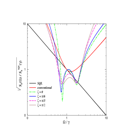
FIG. 3.: Log-log plot of $\sqrt{S_{h}(\Omega)/S^{\rm SQL}_{h}(\gamma)}$ versus $\Omega/\gamma$ for the following choices of the frequency independent homodyne phase: $\zeta=0$, $\zeta=\pi/6$, $\zeta=\pi/3$ and $\zeta=\pi/2$, with $\rho=0.9$, $\phi=\pi/2-0.47$ and $I_{o}=I_{\rm SQL}$. The plot also shows the noise curve for a conventional interferometer and the SQL line. For LIGO-II, $\gamma=2\pi\times 100\,{\rm Hz}$ (top axis) and $\sqrt{S_{h}^{\rm SQL}(\gamma)}=2\times 10^{-24}\,{\rm Hz}^{-1/2}$.

The sensitivity curves for the two quadratures go substantially below the SQL and show two interesting resonant valleys. In Fig. 3 we plot the noise curves $\sqrt{S_{h}(\Omega)}$ for different values of the frequency independent homodyne angle $\zeta$, choosing the same parameters used in Fig. 2, i.e. $\rho=0.9$, $\phi=\pi/2-0.47$ and $I_{o}=I_{\rm SQL}$. Note that the location of the resonant dips does not depend much on the angle $\zeta$. This property is confirmed analytically in Sec. IV in the case of a highly-reflecting SR mirror, by an analysis that elucidate the underlying physics.

Before ending this section, let us give an idea of the performances achievable in a SR interferometer if its thermal noise can be made negligible [15]. We have estimated the signal-to-noise ratio for inspiraling binaries, which are among the most promising sources for the detection of GW with earth-based interferometers. The square of the signal-to-noise ratio for a binary system made of black holes and/or neutron stars is given by:

$$\left(\frac{S}{N}\right)^{2}=4\int_{0}^{+\infty}\frac{|h(f)|^{2}}{S_{h}(f)}\,df\,.$$ (41)

Using the Newtonian quadrupole approximation, for which the waveform’s Fourier transform is $|h(f)|^{2}\propto f^{-7/3}$, and introducing in the above integral a lower cutoff due to seismic noise at $\Omega_{s}=0.1\gamma$ ($f_{s}\simeq 10$ Hz), we get for the parameters used in Fig. 2:

$$\frac{({S}/{N})_{1}}{({S}/{N})_{\rm conv}}\simeq 1.83\,,\quad\quad\frac{({S}/{N})_{2}}{({S}/{N})_{\rm conv}}\simeq 1.98\,,$$ (42)

where $({S}/{N})_{1}$, $({S}/{N})_{2}$ and $({S}/{N})_{\rm conv}$ use for the noise spectral density either that of the first quadrature $b_{1}^{\cal C}$ or the second quadrature $b_{2}^{\cal C}$ or the conventional interferometer, respectively. A more thorough analysis of signal-to-noise ratio for inspiraling binaries inevitably requires the specification of the readout scheme and we plan to publish it elsewhere [24].

B Effective shot noise and radiation-pressure noise

In this section we shall discuss the crucial role played by shot-noise / radiation-pressure correlations that are present in LIGO-II’s quadrature outputs (21) and noise spectral densities (37), in beating the SQL. Our analysis is based on the general formulation of linear quantum measurement theory developed by Braginsky and Khalili [4] and assumes also the results obtained in [16], [11].

To identify the radiation pressure and the shot noise contributions in the total optical noise, we use the fact that they transform differently under rescaling of the mirror mass. Indeed, it is straightforward to show that in the total optical noise there exist only two kinds of terms. There are terms that are invariant under rescaling of the mass and terms that are proportional to $1/m$. Hence, quite generally we can rewrite the output ${\cal O}$ of the whole optical system as [4], [11]

$${\cal O}(\Omega)={\cal Z}(\Omega)+{\cal R}_{xx}(\Omega)\,{\cal F}(\Omega)+L\,h(\Omega)\,,$$ (43)

where by output we mean one of the two quadratures $b_{1}^{\cal C}$, $b_{2}^{\cal C}$ or a combination of them, e.g., $b_{\zeta}^{\cal C}$ (modulo a normalization factor) and where ${\cal R}_{xx}$ is the susceptibility of the antisymmetric mode of motion of the four mirrors [4], given by

$${\cal R}_{xx}(\Omega)=-\frac{4}{m\,\Omega^{2}}\,.$$ (44)

The observables ${\cal Z}$ and ${\cal F}$ in Eq. (43) do not depend on the mirror masses $m$, and satisfy the commutation relations (Eq. (2.19) in Ref. [11])

$$[{\cal F}(\Omega),{\cal F}^{\dagger}(\Omega^{\prime})]=0=[{\cal Z}(\Omega),{\cal Z}^{\dagger}(\Omega^{\prime})]\,,\quad\quad[{\cal Z}(\Omega),{\cal F}^{\dagger}(\Omega^{\prime})]=-2\pi i\hbar\delta(\Omega-\Omega^{\prime})\,.$$ (45)

We shall refer to ${\cal Z}$ and ${\cal F}$ as the effective shot noise and effective radiation-pressure force, respectively, because we have shown [11] that for a SR interferometer the real back-action force acting on the test masses is not proportional to the effective radiation-pressure noise, but instead is a combination of the two effective observables ${\cal Z}$ and ${\cal F}$. When the shot noise and radiation-pressure noise are correlated, the real back-action force does not commute with itself at different times, which makes the analysis in terms of real quantities more complicated than in terms of the effective ones. We prefer to discuss our results in terms of real quantities separately [11], in a more formal context which uses the description of a GW interferometer as a linear quantum-measurement device [4].

The noise spectral density, written in terms of the effective operators ${\cal Z}$ and ${\cal F}$, reads [4]:

$$S_{h}=\frac{1}{L^{2}}\,\left\{S_{{\cal Z}{\cal Z}}+2{\cal R}_{xx}\,\Re\left[S_{{\cal F}{\cal Z}}\right]+{\cal R}_{xx}^{2}\,S_{{\cal F}{\cal F}}\right\}\,,$$ (46)

where the (one-sided) cross spectral density of two operators is expressible, by analogy with Eq. (35), as

$$\frac{1}{2}\,S_{{\cal A}{\cal B}}(\Omega)2\pi\,\delta\left(\Omega-\Omega^{\prime}\right)=\frac{1}{2}\,\langle{\cal A}(\Omega){\cal B}^{\dagger}(\Omega^{\prime})+{\cal B}^{\dagger}(\Omega^{\prime}){\cal A}(\Omega)\rangle\,.$$ (47)

In Eq. (46) the terms containing $S_{{\cal Z}{\cal Z}}$, $S_{{\cal F}{\cal F}}$ and $\Re\left[S_{{\cal F}{\cal Z}}\right]$ should be identified as effective shot noise, back-action noise and a term proportional to the effective correlation between the two noises, respectively [4]. Relying on the commutators (45) between the effective field operators one can derive [4], [11] the following uncertainty relation for the (one-sided) spectral densities and cross correlations of ${\cal Z}$ and ${\cal F}$:

$$S_{{\cal Z}{\cal Z}}\,S_{{\cal F}{\cal F}}-S_{{\cal Z}{\cal F}}\,S_{{\cal F}{\cal Z}}\geq\hbar^{2}\,.$$ (48)

Equation  (48) does not, in general, impose a lower bound on the noise spectral density Eq. (46). However, in a very important type of measurement it does, namely for interferometers with uncorrelated shot noise and back-action noise, e.g., LIGO-I/TAMA/Virgo. In this case $S_{{\cal Z}{\cal F}}=0=S_{{\cal F}{\cal Z}}$ [7] and inserting the vanishing correlations into Eqs. (47), (48), one easily finds that the noise spectral density has a lower bound which is given by the standard quantum limit, i.e.

$$S_{h}(\Omega)\geq S_{h}^{\rm SQL}(\Omega)\equiv\frac{2\left|R_{xx}(\Omega)\right|\hbar}{L^{2}}=\frac{8\hbar}{m\Omega^{2}\,L^{2}}=h_{\rm SQL}^{2}(\Omega)\,.$$ (49)

From this it follows that to beat the SQL one must create correlations between shot noise and back-action noise.

Before investigating those correlations in a SR inteferometer, we shall first show how such correlations can be built up statically in a conventional (LIGO-I/TAMA/Virgo) interferometer by implementing frequency-independent homodyne detection at some angle $\zeta$  [8], [7]. By identifying in the interferometer output (38) the terms independent of $m$ as effective shot noise and those inversely proportional to $m$ as effective back-action noise, we get the effective field operators ${\cal Z}^{\rm conv}_{\zeta}$ and ${\cal F}^{\rm conv}_{\zeta}$:

$${\cal Z}^{\rm conv}_{\zeta}(\Omega)=\frac{e^{i\beta}\,L\,h_{\rm SQL}}{\sqrt{2{\cal K}}}\,\left(a_{2}+a_{1}\,\tan\zeta\right)\,,\quad\quad{\cal F}^{\rm conv}_{\zeta}(\Omega)=\frac{\hbar\,e^{i\beta}\,\sqrt{2{\cal K}}}{L\,h_{\rm SQL}}\,a_{1}\,.$$ (50)

[We remind the readers that $h_{\rm SQL}\propto 1/\sqrt{m}$ and that ${\cal K}\propto 1/m$.] Evaluating the spectral densities of those operators using Eqs. (47) and (36), we obtain the following expressions for the spectral densities and their static correlations:

$$S^{\rm conv}_{{\cal Z}_{\zeta}{\cal Z}_{\zeta}}(\Omega)=\frac{L^{2}\,h_{\rm SQL}^{2}}{2{\cal K}}\,(1+\tan^{2}\zeta)\,,\quad\quad S^{\rm conv}_{{\cal F}_{\zeta}{\cal F}_{\zeta}}(\Omega)=\frac{2{\cal K}\,\hbar^{2}}{L^{2}\,h_{\rm SQL}^{2}}\,,\quad\quad S^{\rm conv}_{{\cal Z}_{\zeta}{\cal F}_{\zeta}}(\Omega)=\hbar\,\tan\zeta=S^{\rm conv}_{{\cal F}_{\zeta}{\cal Z}_{\zeta}}(\Omega)\,.$$ (51)

By inserting these in Eq. (46) and optimizing the coupling constant ${\cal K}$, we see that the SQL can be beaten for any $0<\zeta<\pi/2$, i.e. whenever there are nonvanishing correlations. See Refs. [7] and [8] for further details.

Let us now derive the correlations between shot noise and back action noise in SR interferometers. Because in this case the correlations are built up dynamically by the SR mirror and are present in all quadratures, as an example, we limit ourselves to the two quadratures $b^{\cal C}_{1}$ and $b^{\cal C}_{2}$. Identifying in Eqs. (33), (34) the effective shot and back-action noise terms due to their $m$ dependences, we obtain the effective field operators ${\cal Z}_{1}$, ${\cal Z}_{2}$, ${\cal F}_{1}$ and ${\cal F}_{2}$

$${\cal Z}_{1}(\Omega)=-\frac{e^{i\beta}\,L\,h_{\rm SQL}}{\sqrt{2{\cal K}}}\,\frac{\left[a_{1}\,(-2\rho\,\cos 2\beta+(1+\rho^{2})\,\cos 2\phi)+a_{2}\,(-1+\rho^{2})\,\sin 2\phi\right]\,\csc\phi}{\tau\,(1+e^{2i\beta}\,\rho)}\,,$$ (52)

$${\cal Z}_{2}(\Omega)=-\frac{e^{i\beta}\,L\,h_{\rm SQL}}{\sqrt{2{\cal K}}}\,\frac{\left[a_{1}\,(1-\rho^{2})\,\sin 2\phi+a_{2}\,(-2\rho\,\cos 2\beta+(1+\rho^{2})\,\cos 2\phi)\right]\,\sec\phi}{\tau\,(-1+e^{2i\beta}\,\rho)}\,,$$ (53)

and

$${\cal F}_{1}(\Omega)=\frac{\hbar\,e^{i\beta}\,\sqrt{2{\cal K}}}{L\,h_{\rm SQL}}\,\frac{\left[a_{1}\,(1+\rho^{2})\,\cos\phi+a_{2}\,(-1+\rho^{2})\,\sin\phi\right]}{\tau\,(1+e^{2i\beta}\,\rho)}\,,$$ (54)

$${\cal F}_{2}(\Omega)=\frac{\hbar\,e^{i\beta}\,\sqrt{2{\cal K}}}{L\,h_{\rm SQL}}\,\frac{\left[a_{1}\,(-1+\rho^{2})\,\cos\phi+a_{2}\,(1+\rho^{2})\,\sin\phi\right]}{\tau\,(-1+e^{2i\beta}\,\rho)}\,.$$ (55)

Evaluating the spectral densities of the above operators through Eqs. (47) and (36) we obtain the following expressions:

$$S_{{\cal F}_{1}{\cal F}_{1}}(\Omega)=\frac{\hbar^{2}\,2{\cal K}}{L^{2}\,h_{\rm SQL}^{2}}\,\frac{1+\rho^{4}+2\rho^{2}\cos\phi}{{(1-\rho^{2})\,(1+\rho^{2}+2\rho\,\cos 2\beta)}}\,,$$ (56)

$$S_{{\cal F}_{2}{\cal F}_{2}}(\Omega)=\frac{\hbar^{2}\,2{\cal K}}{L^{2}\,h_{\rm SQL}^{2}}\,\frac{1+\rho^{4}-2\rho^{2}\cos\phi}{{(1-\rho^{2})\,(1+\rho^{2}-2\rho\,\cos 2\beta)}}\,,$$ (57)

and

$$S_{{\cal Z}_{1}{\cal Z}_{1}}(\Omega)=\frac{L^{2}\,h_{\rm SQL}^{2}}{2{\cal K}}\frac{\left[4(-1+\rho^{2})^{2}\,\cos^{2}\phi+(-2\rho\,\cos 2\beta+(1+\rho^{2})\,\cos 2\phi)^{2}\,\csc^{2}\phi\right]}{(1-\rho^{2})\,(1+\rho^{2}+2\rho\,\cos 2\beta)}\,,$$ (58)

$$S_{{\cal Z}_{2}{\cal Z}_{2}}(\Omega)=\frac{L^{2}\,h_{\rm SQL}^{2}}{2{\cal K}}\frac{\left[4(-1+\rho^{2})^{2}\,\sin^{2}\phi+(-2\rho\,\cos 2\beta+(1+\rho^{2})\,\cos 2\phi)^{2}\,\sec^{2}\phi\right]}{(1-\rho^{2})\,(1+\rho^{2}-2\rho\,\cos 2\beta)}\,.$$ (59)

Finally, for the correlations between the shot noise and back-action noise we get:

$$S_{{\cal F}_{1}{\cal Z}_{1}}(\Omega)=S_{{\cal Z}_{1}{\cal F}_{1}}(\Omega)=-\frac{\hbar\,\left[(-1+\rho^{2})^{2}-2\rho\,(1+\rho^{2})\,\cos 2\beta+4\rho^{2}\,\cos 2\phi\right]\,\cot\phi}{(1-\rho^{2})\,(1+\rho^{2}+2\rho\,\cos 2\beta)}\,,$$ (60)

$$S_{{\cal F}_{2}{\cal Z}_{2}}(\Omega)=S_{{\cal Z}_{2}{\cal F}_{2}}(\Omega)=\frac{\hbar\,\left[(-1+\rho^{2})^{2}+2\rho\,(1+\rho^{2})\,\cos 2\beta-4\rho^{2}\,\cos 2\phi\right]\,\tan\phi}{(1-\rho^{2})\,(1+\rho^{2}-2\rho\,\cos 2\beta)}\,.$$ (61)

These correlations depend on the sideband angular frequency $\Omega$ and are generically different from zero. However, when $\phi=0$ and $\phi=\pi/2$ the correlations are zero. We shall analyze these two extreme configurations in the following section.

C Two special cases: extreme signal-recycling and resonant-sideband-extraction configurations

In this section we discuss two extreme cases that are well known and have been much investigated in the literature using a semiclassical analysis [13, 14]. In these two cases the dynamical correlations between shot noise and radiation-pressure noise are zero. This has two implications: (i) the semiclassical analysis and predictions [13, 14] are correct (when straightforwardly complemented by radiation pressure noise), and (ii) the noise curves are always above the SQL. Of course, static correlations can always be introduced by measuring the quadrature $b_{\zeta}$. In these two extreme cases there are no instabilities and the input–output relation of the SR interferometer can be obtained from the conventional noise by just rescaling the parameter ${\cal K}$ [Eq. (14)].

1 Extreme signal-recycling (ESR) configuration: $\phi=0$

For $\phi=0$, the gravitational-wave signal appears only in the second quadrature $b_{2}$ but not in the first quadrature $b_{1}$ (see Eq. (29) with $\zeta=0$ and $\pi/2$, respectively). Defining

$$\widetilde{{\cal K}}\equiv\frac{{\cal K}\,\tau^{2}}{1+\rho^{2}-2\rho\,\cos{2\beta}}\,,$$ (62)

it is straightforward to deduce that the spectral density of the noise takes the simple form

$$S^{\rm ESR}_{h}=\frac{S_{h}^{\rm SQL}}{2}\,\left(\frac{1}{\widetilde{{\cal K}}}+\widetilde{{\cal K}}\right)\,.$$ (63)

In the left panel of Fig. 4 we plot $\sqrt{S_{h}^{\rm ESR}(\Omega)/S_{h}^{\rm SQL}(\gamma)}$ versus $\Omega/\gamma$ for different choices of the reflectivity $\rho$. As we vary the reflectivity of the SR mirror the minimum of the various curves is shifted along the SQL line, and the shape of the noise curve change a bit because both ${\cal K}$ and $\beta$ in Eqs. (62), (63) depend on frequency. Moreover, for $\Omega/\gamma\gg 1$ and $\Omega/\gamma\ll 1$ the curves are well above the conventional interferometer noise. This effect becomes worse and worse as $\rho\rightarrow 1$ and is described by the formulas

$$\frac{S^{\rm ESR}_{h}(\Omega)}{S_{h}^{\rm SQL}(\gamma)}\rightarrow\frac{1}{4}\frac{\Omega^{2}}{\gamma^{2}}\,\left(\frac{1+\rho}{1-\rho}\right)\,\frac{I_{\rm SQL}}{I_{o}}\,,\quad\quad\frac{\Omega}{\gamma}\gg 1\,;\quad\quad\frac{S^{\rm ESR}_{h}(\Omega)}{S_{h}^{\rm SQL}(\gamma)}\rightarrow\frac{\gamma^{4}}{\Omega^{4}}\,\left(\frac{1+\rho}{1-\rho}\right)\,\frac{I_{o}}{I_{\rm SQL}}\,,\quad\quad\quad\frac{\Omega}{\gamma}\ll 1\,.$$ (64)

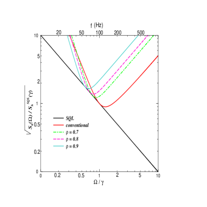
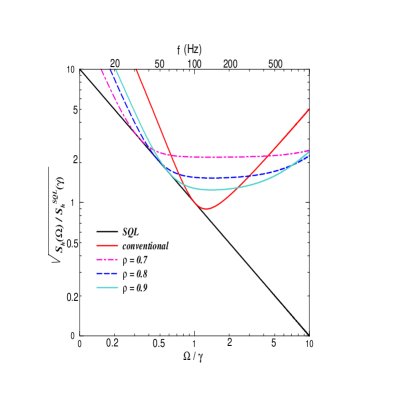
FIG. 4.: Log-log plot of $\sqrt{S_{h}^{\rm ESR}(\Omega)/S_{h}^{\rm SQL}(\gamma)}$ versus $\Omega/\gamma$ for the extreme signal-recycling configuration (left panel) $\phi=0$ with $\rho=0.7$, $\rho=0.8$, $\rho=0.9$ and $I_{o}=I_{\rm SQL}$ and for the extreme resonant-sideband-extraction configuration (right panel) $\phi=\pi/2$ with $\rho=0.7$, $\rho=0.8$ and $\rho=0.9$, with $I_{o}=I_{\rm SQL}$. Also plotted for comparison are the noise curve for a conventional interferometer and the SQL line. For further detail on these well known configurations, see Refs. [13, 14].

The signal-to-noise ratio for inspiraling binaries is given in this case (for $\rho=0.9$, $I_{o}=I_{\rm SQL}$) by:

$$\frac{({S}/{N})_{\rm ESR}}{({S}/{N})_{\rm conv}}\simeq 0.73\,.$$ (65)

Hence, this LIGO-II configuration ($\phi=0$) is not appealing. The noise curves could be better than the ones for a conventional interferometer in the range $\sim\!20-60$ Hz, depending on the value of $\rho$, but they get worse everywhere else, and overall, for any $\rho$ the signal-to-noise ratio for inspiraling binaries is lower than in the case of a conventional interferometer.

2 Extreme resonant-sideband-extraction (ERSE) configuration: $\phi=\pi/2$

For $\phi={\pi}/{2}$, using Eq. (29) with $\zeta=\pi/2$, we find that only the first quadrature $b_{1}$ contains the gravitational-wave signal. Introducing

$$\overline{{\cal K}}\equiv\frac{{\cal K}\,\tau^{2}}{1+\rho^{2}+2\rho\,\cos{2\beta}}\,,$$ (66)

(which depends on frequency through both ${\cal K}$ and $\beta$), we easily deduce that the noise spectral density reads

$$S_{h}^{\rm ERSE}=\frac{S_{h}^{\rm SQL}}{2}\,\left(\frac{1}{\overline{{\cal K}}}+\overline{{\cal K}}\right)\,.$$ (67)

The right panel of Fig. 4 shows $\sqrt{S_{h}^{\rm ERSE}(\Omega)/S_{h}^{\rm SQL}(\gamma)}$ as a function of $\Omega/\gamma$ for different values of the reflectivity $\rho$. As for the ESR configuration discussed above, when we vary the reflectivity of the SR mirror the minimum of the various curves moves along the SQL line. But by contrast with the ESR configuration, for $\Omega/\gamma\gg 1$ and $\Omega/\gamma\ll 1$ the curves are significantly below the conventional-interferometer noise. This effect becomes better and better as $\rho\rightarrow 1$ and is described by the asymptotic limits

$$\frac{S^{\rm ERSE}_{h}(\Omega)}{S_{h}^{\rm SQL}(\gamma)}\rightarrow\frac{1}{4}\frac{\Omega^{2}}{\gamma^{2}}\,\left(\frac{1-\rho}{1+\rho}\right)\,\frac{I_{\rm SQL}}{I_{o}}\,,\quad\quad\frac{\Omega}{\gamma}\gg 1\,;\quad\quad\frac{S^{\rm ERSE}_{h}(\Omega)}{S_{h}^{\rm SQL}(\gamma)}\rightarrow\frac{\gamma^{4}}{\Omega^{4}}\,\left(\frac{1-\rho}{1+\rho}\right)\,\frac{I_{o}}{I_{\rm SQL}}\,,\quad\quad\frac{\Omega}{\gamma}\ll 1\,.$$ (68)

In conclusion, in the ERSE configuration ($\phi={\pi}/{2}$), the situation is in some sense the reverse of the ESR scheme ($\phi=0$). In the former the bandwidths are much larger than in either the ESR of the conventional interferometer. However, the more broadband curves are obtained at the cost of losing sensitivity in the frequency range $\sim\!70-250$ Hz and this explains why the maximum signal-to-noise ratio for inspiraling binaries,

$$\frac{({S}/{N})_{\rm ERSE}}{({S}/{N})_{\rm conv}}\simeq 1.096\,\quad\quad{\rm for}\quad\rho=0.48\quad{\rm and}\quad I_{o}=I_{\rm SQL}\,.$$ (69)

is not very different from that of a conventional interferometer. Finally, let us observe that our two extreme cases are linked mathematically by taking $\rho\rightarrow\ -\rho$ ( $\overline{{\cal K}}\rightarrow\widetilde{{\cal K}}$) and exchanging the two quadratures. For much further analysis and detail of the ERSE and ESR configurations, see Refs. [13, 14].

IV Structure of resonances and instabilities

We now turn our attention from the well known extreme configurations, for which previous analysis gave correct predictions, to the more general case $0<\phi<\pi/2$. As Figs. 2, 3 show, the noise curves for a SR interferometer with frequency independent homodyne detection generically exhibit resonant features that vary as $I_{o}$, $\rho$, $\phi$ and $\zeta$ are changed. These resonances are closely related to the optical-mechanical resonances of the dynamical system formed by the optical field and the mirrors. A thorough study of this system must investigate explicitly the motion of the mirrors, instead of including it implicitly in the formulae as we did in this paper. It can be most clearly worked out using the formalism of linear quantum measurements [4], which we have recently extended to SR interferometers [11]. In this section, we limit our investigation to the resonant structures in the amplitudes of the optical fields, and for simplicity we work in the limit of a totally reflecting SR mirror, i.e. $\rho=1$. This limit provides simple analytical expressions for the resonant frequencies as functions of the SR detuning phase $\phi$ and the light power $I_{o}$. We shall comment on the general case $\rho\neq 1$, which we have tackled at length in Ref. [11], only at the end of this section.

A Resonances of the closed system: $\rho=1$

We shall investigate the free oscillation modes of the whole interferometer when the GW signal is absent [$h(\Omega)=0$] and there is no output field ($\rho=1$), so the system is closed. We consider the regime of classical electrodynamics, i.e. we work with the two classical quadrature fields $E_{1}$ and $E_{2}$, satisfying the same equations of motion as the quantum-field operators $c_{1}$ and $c_{2}$ (see Fig. 1). We shall evaluate the stationary modes, notably the eigenmodes and eigenvalues of the whole optico-mechanical system made of the end mirrors and the signal recycled optical field. We achieve this by propagating the in-going fields $E_{1}$ and $E_{2}$ (entering the beam splitter’s dark port) into the conventional interferometer, along a complete round trip, and then through the SR cavity back to the starting point. The round-trip propagation leads to the following homogeneous equation for the eigenmodes:

$$\left[\left(\matrix{\cos 2\phi&-\sin 2\phi\cr\sin 2\phi&\cos 2\phi}\right)e^{2i\beta}\left(\matrix{1&0\cr-{\cal{K}}&1}\right)-{\rm I}\right]\left(\matrix{E_{1}\cr E_{2}}\right)=0\,,$$ (70)

which can be simplified into the more interesting form:

$$T\left(\matrix{e^{2i(\alpha+\beta)}-1\cr 0&e^{2i(-\alpha+\beta)}-1}\right)T^{-1}\left(\matrix{E_{1}\cr E_{2}}\right)=0\,,\quad\quad 2\alpha\equiv\arccos\left(\cos 2\phi+\frac{\cal K}{2}\sin 2\phi\right)\,,$$ (71)

where $T$ is a matrix whose precise form is unimportant. Note that the definition of the function $\arccos$ ensures that $\Re(2\alpha)$ ranges from $0$ to $\pi$. The free oscillation condition is then given by:

$$\cos 2\beta_{\rm res.}=\cos 2\alpha=\cos 2\phi+\frac{\cal K}{2}\sin 2\phi\,.$$ (72)

Solving Eq. (72) explicitly in terms of the frequency $\Omega$, we obtain the rather simple analytical equation for the position of the resonances:

$$\frac{\Omega^{2}_{\rm res.}}{\gamma^{2}}=\frac{1}{2}\left[\tan^{2}\phi\pm\sqrt{\tan^{4}\phi-\frac{4I_{o}}{I_{\rm SQL}}\,\tan\phi}\right]\,.$$ (73)

This equation is characterized by three regimes ($0<\phi<\pi$):

• $\phi>\pi/2$: one real and one imaginary resonant frequency;

• $\arctan[(4I_{o}/I_{\rm SQL})^{1/3}]<\phi<\pi/2$: two real resonant frequencies;

• $0<\phi<\arctan[(4I_{o}/I_{\rm SQL})^{1/3}]$: two complex conjugate resonant frequencies.

Equation (73) is very similar to the resonance equation that Braginsky, Gorodetsky and Khalili have derived for their proposal “Optical bar gravitational wave detectors” (see Appendix D of Ref. [9]).

For very low light power, ${I_{o}}\ll{I_{\rm SQL}}$, the second term under the square root on the RHS of Eq. (73) goes to $0$ and the four roots tend to $\Omega=0$ (double root) and $\Omega=\pm\gamma\tan\phi$. We interpret this limit as follows (see Ref. [11] for further details): When the coupling between the motion of the mirror and the optical field is zero ($I_{o}\rightarrow 0$), the resonant frequencies of the entire system are given by the resonances of the test mass, i.e. the free-oscillation modes of a test mass ($\Omega=0$), plus the resonances of the optical field, i.e. the electromagnetic modes of the entire cavity with fixed mirrors, given by $\Omega=\pm\gamma\tan\phi$ [13]. When the light power is increased toward $I_{\rm SQL}$, the coupling between the free test mass and the optical field drives the four resonant frequencies away from their decoupled values. By analyzing the four coupled resonant frequencies, we can easily identify the ones with the $-$ ($+$) sign in Eq. (73) as remnants of the resonant frequencies of the free test mass (optical field). (For a more thorough discussion of these results see Ref. [11], where we explicitly examine the mirror motion.)

Let us observe that Eq. (72) can also be obtained as follows. By expanding the noise spectral density (37) for $\tau\rightarrow 0$, we get:

$$\frac{S_{h}(\Omega)}{h^{2}_{\rm SQL}(\Omega)}=\frac{{\left(-2\,\cos 2\,\beta+2\,\cos 2\,\phi+{\cal K}\,\sin 2\,\phi\right)}^{2}}{8\,{\cal K}\,\left[\cos^{2}\beta\,(\sin^{2}\zeta-\cos^{2}\phi)+\cos^{2}\phi\,\cos^{2}\zeta\right]}\,\frac{1}{\tau^{2}}+{\cal O}(\tau^{0})\,.$$ (74)

The leading term of the expansion goes to zero when $2\cos{2\phi}-2\cos{2\beta_{\rm res.}}+{\cal K}\sin{2\phi}=0$, which is exactly the resonant condition (72) for the closed system derived above. This means that for (open) SR interferometers with highly reflecting SR mirrors, the dips in the noise curves agree with the resonances of the closed system.

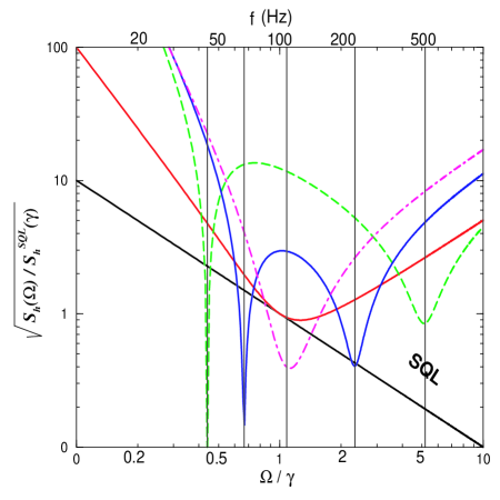
FIG. 5.: Log-log plot of $\sqrt{S_{h}(\Omega)/S_{h}^{\rm SQL}(\gamma)}$ versus $\Omega/\gamma$ for $I_{o}=I_{\rm SQL}$, $\rho=0.95$ and $\zeta=0$ (i.e. the second quadrature $b_{2}^{\cal C}$ is measured). The detuning phase $\phi$ takes the values (going from right to left): $\pi/2-0.19$, $\pi/2-0.39$ and $\pi/2-0.59$. The vertical grid lines have been drawn by using Eq. (73) and taking the real part of $\Omega_{\rm res.}$. These lines agree well with the positions of the resonant dips.

In practice, the real part of the resonant frequencies  (73) for the closed system turns out to be a good approximation to the positions of the valleys in the noise spectral density of an (open) SR interferometer with high SR-mirror reflectivity. To illustrate this fact, in Fig. 5 we plot the noise curves $\sqrt{S_{h}(\Omega)}$ for the second quadrature $b_{2}^{\cal C}$ with $I_{o}=I_{\rm SQL}$, $\rho=0.95$ and varying $\phi$. The vertical lines have been drawn by solving Eq. (73) numerically for $\Omega$ and taking its real part, i.e., the real part of the resonant frequencies of the closed systems. There is indeed very good agreement. This suggests that the gain in sensitivity comes from a resonant amplification effect; see the discussion at the end of the Sec. IV C.

If the imaginary part of the resonant frequency is positive (negative) then, with our convention for the Fourier transform, the solution is unstable (stable). The best noise sensitivity curves have detuning phase $\phi$ in the range $\arctan[(4I_{o}/I_{\rm SQL})^{1/3}]\,\raise 1.72218pt\hbox{$<$}\kern-8.00003pt\lower 2.6694pt\hbox{$\sim$}\,\phi\,\raise 1.72218pt\hbox{$<$}\kern-8.00003pt\lower 2.6694pt\hbox{$\sim$}\,\pi/2$, which for $\rho=1$ correspond to two real resonant frequencies, and no instability. However, as soon as we allow the transmissivity of the SR mirror $\tau$ to be different from zero (as it must be in a real interferometer), we always find that one of the two resonant frequencies has a positive imaginary part [11]. A more detailed analysis of the dynamics of the system has shown that this is a rather weak instability which typically develops on a time scale of $\raise 1.72218pt\hbox{$<$}\kern-8.00003pt\lower 2.6694pt\hbox{$\sim$}\,0.1\gamma$ and can be cured by introducing an appropriate control system [11].

B Semiclassical interpretation of resonances for small $\cal K$: pure optical resonances

In this section we shall focus on the optical-field resonances and shall relate our results to previous semiclassical analyses of SR interferometers [13, 14].

The test-mass motion affects the optical fields through the term ${\cal K}=2\left(I_{o}/I_{\rm SQL}\right)\gamma^{4}/\left(\Omega^{2}(\Omega^{2}+\gamma^{2})\right)$, where the factor $I_{o}/I_{\rm SQL}$ can be considered a measure of the strength of the coupling. The quantity $\cal K$ governs both the resonant condition and the relative magnitude of shot noise and radiation-pressure noise. In particular, when ${\cal K}$ is very small, Eq. (72) simplifies to $\cos{2\phi}-\cos{2\beta_{\rm res.}}=0$, which can be solved easily, giving:

$$2(\pm\beta_{\rm res.}+\phi)=2\pi\,n\,,\quad\quad{\rm i.e.}\quad\Omega_{\rm res.}=\pm\gamma\tan\phi\,,$$ (75)

with $n$ an integer. Equation (75) can be explained with a simple optics argument: The quantity $\pm 2\beta$ is the phase gained by the upper and lower GW sidebands while in an arm cavity, while $\phi$ is the phase gained when traveling one way down the SR cavity. Thus $2(\pm\beta+\phi)$ is just the round-trip phase, and Eq. (75) is the resonant condition for the entire (closed) interferometer. Hence, the presence of $\cal K$ in the resonant condition (72) provides the deviation from a pure optical resonance. Moreover, $\cal K$ is also an indicator of the different scalings of $I_{o}$ and $m$ in the final expressions for the noises, and therefore it governs the relative magnitude of the shot noise and radiation-pressure noise – the smaller the $\cal K$, the more important the shot noise compared to radiation pressure noise. When $\cal K$ is small, a semi-classical argument helps to explain the features of our noise curves. If we are close to the resonance, then feeding back the signal at that frequency increases the peak sensitivity while decreasing the bandwidth. Different schemes of such narrow-banding have been proposed, e.g., see Drever [29]. The scheme discussed here, in which the signal at the dark port is fed back into the arm cavities, is called signal recycling (in the narrower sense), and was invented by Meers [13]. If, on the other hand, we are far enough from the resonances, sideband signals are not encouraged to go back into the interferometer; in particular, at $|\beta_{\text{anti-res.}}|\simeq|\beta_{\rm res.}\pm\pi/2|$, there is antiresonance, and the signal is encouraged to go out. This is what is generally called resonant sideband-extraction and was invented by Mizuno [14], see Sec. III C. The range in between, $\beta_{\rm res.}<\beta<\beta_{\text{anti-res.}}$, is called ‘detuned’ signal recycling and has recently been demonstrated experimentally on the 30 m laser interferometer at Garching, Germany by Freise et al. [30] and at Caltech on a table-top experiment by Mason [31].

As an example of resonance (not anti-resonance), we plot in Fig. 6 the spectral density $S_{h}(\Omega)$ when the second quadrature $b_{2}^{\cal C}$ is measured, for very low light power $I_{o}=10^{-4}\,I_{\rm SQL}$ and high reflectivity $\rho=0.95$, and for various values of the detuning phase $\phi$. The vertical grid lines in Fig. 6 are drawn according to Eq. (75) and indeed, there is excellent agreement.

It is interesting to note that although for LIGO-II $I_{o}=I_{\rm SQL}$, there is still a frequency band where $\cal K$ is relatively small. This is due to the fact that $\cal K$ drops very fast as $\Omega$ increases. In that frequency band the semiclassical formalism gives a correct result for the optical resonances [28]. However, since the semiclassical approach does not take into account the motion of the arm-cavity end mirrors, it can only describe one resonance (and not two) in the entire spectrum.

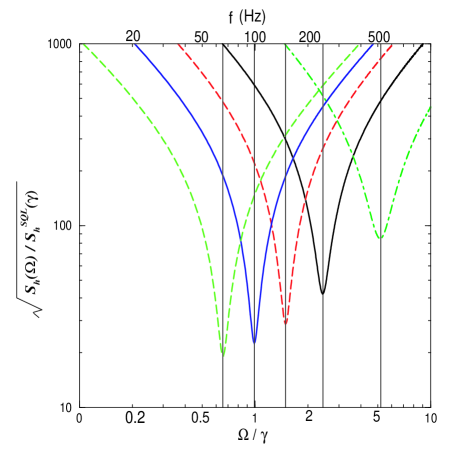
FIG. 6.: Log-log plot of $\sqrt{S_{h}(\Omega)/S_{h}^{\rm SQL}(\gamma)}$ versus $\Omega/\gamma$ for $\zeta=0$ (i.e. $b_{2}^{\cal C}$ is measured) and for extremely low light power and high reflectivity: $I_{o}=10^{-4}I_{\rm SQL}$ and $\rho=0.95$. $\phi$ takes the values (going from right to left): $\pi/2-0.19$, $\pi/2-0.39$, $\pi/2-0.59$, $\pi/2-0.79$ and $\pi/2-0.99$. A series of resonances appear whose positions agree with the vertical grid lines drawn according to ${\Omega_{\rm res.}}/{\gamma}=|\tan\phi|$ [Eq. (75)].

C Quantum mechanical discussion of the general case: two resonances and $\rho\neq 1$

The correspondence between the optical-mechanical resonances and the minima of the noise curves suggests that the gain in sensitivity comes from a resonant amplification of the input signal, i.e. of the gravitational force acting on the mirrors, as already observed for optical bar GW detectors by Braginsky’s group [9]. Let us discuss this point more deeply.

The quantum part of the input–output relation  (21) (with $|\Phi|\ll 1$ as we have assumed throughout this paper) reads

$$b_{i}^{\rm quant}=\frac{e^{2i\beta}\,C_{ij}}{M}\,a_{j}\,,\quad\quad i,j=1,2\,.$$ (76)

We find it convenient to renormalize the quantum transfer matrix:

$${\cal M}_{ij}\equiv\frac{C_{ij}}{|M|}\,,\quad\quad i,j=1,2$$ (77)

so $\det{\cal M}_{ij}=1$. Note that this ${\cal M}_{ij}$ is normalized with respect to unit quantum noise. Because the $C_{ij}$ are real, the matrix ${\cal M}$ depends on three real parameters and we can always decompose it into two rotations $R(\theta)$, $R(\varphi)$ and a squeeze $S(r)$ (see for details Ref. [23]), e.g., ${\cal M}=R(\theta)\,R(\varphi)\,{S}(r)\,R(-\varphi)$, with

$$R(\theta)=\left(\matrix{\cos\theta&-\sin\theta\cr\sin\theta&\cos\theta}\right)\,,\quad\quad{S}(r)=\left(\matrix{e^{r}&0\cr 0&e^{-r}}\right)\,,$$ (78)

where the factor $e^{r}$ describes the stretching ($r>0$) or squeezing ($r<0$) of the quantum fluctuations in the quadrature $b_{i}$ [see Eqs. (76), (77)]. Note that classical optical fields always have a zero squeeze factor.

To express the squeeze parameter $r$ in terms of the physical parameters describing the SR interferometer, we simply take the trace of the matrix ${\cal M}\,{\cal M}^{\dagger}$, obtaining

$$e^{2r}+e^{-2r}=2+\frac{\tau^{4}\,{\cal K}^{2}}{|M|^{2}}\,.$$ (79)

Hence, in a SR interferometer the squeezing (generally called ponderomotive squeezing) is induced by the back-action force acting on the mirror through the effective coupling ${\cal K}$. In particular, for small ${\cal K}$, we have $e^{2r}+e^{-2r}\approx 2$ and the squeeze factor $r$ goes to $0$, which means the output field is classical. For our discussion below the specific expressions of $\theta$ and $\varphi$ in terms of the physical parameters are unimportant.

From the previous discussions and the results derived in [11] we have learned that the zeros of $M(\Omega)$ are the resonant frequencies of the optical-mechanical system and the valleys of the noise spectral densities are their real parts. It is straightforward to show that for $\Omega$ equal to the real part of the resonances $|M|\propto\tau^{2}$. Hence, on resonance, for typical values of the physical quantities $I_{o}$, $\rho$ and $\phi$, the RHS of Eq. (79) goes to a constant when $\tau\rightarrow 0$. This means that the squeeze factor $r$ does not grow much around the resonances. On the other hand, the absolute value of the output signal strength [the term involving $h$ in Eq. (21)], is given by

$$\frac{\sqrt{2{\cal K}}\,\tau\,|D_{i}|}{h_{\rm SQL}\,|M|}\,h\,,\quad\quad i=1,2\,,$$ (80)

and because on resonance $1/|M|\!\sim\!1/\tau^{2}$, when $\tau\rightarrow 0$ the classical signal is resonantly amplified and the amplification becomes stronger and stronger as $\tau\rightarrow 0$ (closed system).

This means that, by contrast with QND techniques based on static correlations between shot noise and radiation-pressure noise [7], [8], in SR interferometers the ponderomotive squeezing does not seem to be the major factor that enables the interferometer to beat the SQL. Indeed, whereas the amplitude of the classical output signal is amplified near the resonances, the nonclassical behavior of the output light is not resonantly amplified. Therefore, the beating of the SQL in SR interferometers comes from a resonant amplification of the input signal: the whole system acts like an optical spring, as we have described more thoroughly in [11], and it was also derived for optical bar GW detectors by Braginsky’s group [9].

V Inclusion of losses in signal-recycling interferometers

In this section we shall compute how optical losses affect the noise in a SR inteferometer using the lossy input–output relations for a conventional interferometer [7] and doing a similar treatment of losses in the SR cavity. We shall continue to use our extension of the KLMTV’s formalism as developed in Sec. II. In [11] we show that when losses are included a suitable control system can be implemented to circumvent the instabilities.

KLMTV [7] described the noise that enters the arm cavities of a conventional interferometer at the loss points on the mirrors in terms of a noise operator, whose state is the vacuum, with quadratures $n_{1}$ and $n_{2}$. The resulting lossy input–output relations read [7]

$$d_{1} = c_{1}\,e^{2i\beta}\,\left(1-\frac{{\cal E}}{2}\right)+\sqrt{{\cal E}}\,e^{i\beta}\,n_{1}\,,$$ (81)

$$d_{2} = c_{2}\,e^{2i\beta}\,\left(1-\frac{{\cal E}}{2}\right)+\sqrt{{\cal E}}\,e^{i\beta}\,n_{2}+\sqrt{2{\cal K}}\,\frac{h}{h_{\rm SQL}}\,e^{i\beta}\,\left[1-\frac{\epsilon}{4}\,(3+e^{2i\beta})\right]$$ (83)

$$-{\cal K}\,e^{2i\beta}\,\left\{c_{1}\,\left[1-\frac{\epsilon}{2}\,(3+e^{2i\beta})\right]+\sqrt{\frac{\epsilon}{2}}\,n_{1}\right\}\,,$$

where $\epsilon=2{\cal L}/T$ and ${\cal L}$ is the loss coefficient per round trip in the arm-cavity. For LIGO-II $T$ and ${\cal L}$ are expected to be $T=0.033$ and ${\cal L}\!\sim\!200\times 10^{-6}$, so $\epsilon\!\sim\!0.01$. The quantity ${\cal E}$ which appears in Eqs. (81) and (83) is frequency dependent and is given by

$${\cal E}=\frac{2\epsilon}{1+(\Omega/\gamma)^{2}}\,.$$ (84)

In the present analysis, as in Ref. [7], we do not take into account losses coming from the beam splitter. We expect their effect to be small compared to the losses introduced by the SR cavity and the photodetection process. Fig. 7 sketches the way we have incorporated losses. We describe the loss inside the SR cavity by the fraction of photons lost at each bounce of the interior field off the SR mirror, $\lambda_{\rm SR}$, and we introduce associated noise quantum operators $p_{i}$ ($i=1,2$) into the inward-propagating field operator at the SR mirror (see left panel of Fig. 7). Equations (19) then become

$$e_{1}=\sqrt{1-\lambda_{\rm SR}}\,(\tau\,a_{1}+\rho\,f_{1})+\sqrt{\lambda_{\rm SR}}\,p_{1}\,,\quad\quad e_{2}=\sqrt{1-\lambda_{\rm SR}}\,(\tau\,a_{2}+\rho\,f_{2})+\sqrt{\lambda_{\rm SR}}\,p_{2}\,,$$ (85)

and the noise operators $p_{i}$ satisfy the commutation relations (9). We also assume that the state of $p_{i}$ is the vacuum. We include the losses of the photodetection process in an effective way, by modifying the output field operators and introducing another noise field $q_{i}$ with $i=1,2$ (see right panel of Fig. 7):

$$b^{\rm L}_{1}=\sqrt{1-\lambda_{\rm PD}}\,(\tau\,f_{1}-\rho\,a_{1})+\sqrt{\lambda_{\rm PD}}\,q_{1}\,,\quad\quad b^{\rm L}_{2}=\sqrt{1-\lambda_{\rm PD}}\,(\tau\,f_{2}-\rho\,a_{2})+\sqrt{\lambda_{\rm PD}}\,q_{2}\,.$$ (86)

Here, $\lambda_{\rm PD}$ is the photodetector loss. The noise quadrature fields $q_{i}$ describe additional shot noise due to photodetection and are assumed to satisfy Eq. (9) and to be in the vacuum state. Following the procedure described in Sec. II, we derive from Eqs. (81), (83), (85) and (86) the following input–output relations for the lossy SR interferometer (for simplicity we set $\Phi=0$):

$$\left(\matrix{b^{\rm L}_{1}\cr b^{\rm L}_{2}}\right) = \frac{1}{M^{\rm L}}\left[e^{2i\beta}\,\left(\matrix{C^{\rm L}_{11}&C^{\rm L}_{12}\cr C^{\rm L}_{21}&C^{\rm L}_{22}}\right)\left(\matrix{a_{1}\cr a_{2}}\right)+\sqrt{2{\cal K}}\,\tau\,e^{i\beta}\,\left(\matrix{D^{\rm L}_{1}\cr D^{\rm L}_{2}}\right)\frac{h}{h_{\rm SQL}}+e^{2i\beta}\,\left(\matrix{P_{11}&P_{12}\cr P_{21}&P_{22}}\right)\left(\matrix{p_{1}\cr p_{2}}\right)\right.$$ (88)

$$\left.+e^{2i\beta}\,\left(\matrix{Q_{11}&Q_{12}\cr Q_{21}&Q_{22}}\right)\left(\matrix{q_{1}\cr q_{2}}\right)+e^{2i\beta}\,\left(\matrix{N_{11}&N_{12}\cr N_{21}&N_{22}}\right)\left(\matrix{n_{1}\cr n_{2}}\right)\right]\,,$$

where, to ease the notation, we have defined

$$M^{\rm L} = 1+\rho^{2}\,e^{4i\beta}-2\rho\,\left(\cos{2\phi}+\frac{{\cal K}}{2}\,\sin{2\phi}\right)\,e^{2i\beta}+\lambda_{\rm SR}\,\rho\,\left(-\rho\,e^{2i\beta}+\cos{2\phi}+\frac{{\cal K}}{2}\,\sin{2\phi}\right)\,e^{2i\beta}$$ (90)

$$+\epsilon\,\rho\,\left[2\cos^{2}\beta\,(-\rho\,e^{2i\beta}+\cos 2\phi)+\frac{{\cal K}}{2}\,(3+e^{2i\beta})\,\sin 2\phi\right]\,e^{2i\beta}\,.$$

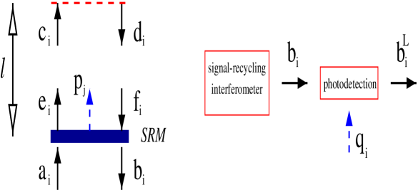
FIG. 7.: Sketchy view of the lossy signal-recycling interferometer. Optical losses in the signal-recycling cavity (on the left) are described by the noise quadratures $p_{i}$, while losses due to the photodetection process (on the right) are included through the noise quadratures $q_{i}$.

Note that $M^{\rm L}$, like $M$ in Eq. (22), has zeros in the lower- and upper-half complex $\Omega$ plane. Hence, the lossy SR interferometer, like the lossless one, also suffers from instabilities. Nevertheless, we have shown in [11] that an appropriate control system can cure them, as in the lossless case. In the following equations we give the various quantities which appear in Eq. (88) accurate to linear order in $\epsilon$ and $\lambda_{\rm SR}$ but to all orders in $\lambda_{\rm PD}$. (We expect $\lambda_{\rm SR}\!\sim\!0.02$ and $\lambda_{\rm PD}\!\sim\!0.1$ [28].) The various quantities read

$$C^{\rm L}_{11} = C^{\rm L}_{22}=\sqrt{1-\lambda_{\rm PD}}\,\left\{(1+\rho^{2})\,\left(\cos{2\phi}+\frac{{\cal K}}{2}\,\sin{2\phi}\right)-2\rho\,\cos{2\beta}\right.$$ (93)

$$\left.-\frac{1}{4}\epsilon\,\left[-2(1+e^{2i\beta})^{2}\,\rho+4(1+\rho^{2})\cos^{2}\beta\,\cos 2\phi+(3+e^{2i\beta})\,{\cal K}\,(1+\rho^{2})\,\sin 2\phi\right]\right.$$

$$+\left.\lambda_{\rm SR}\,\left[e^{2i\beta}\rho-\frac{1}{2}\,(1+\rho^{2})\,\left(\cos{2\phi}+\frac{{\cal K}}{2}\,\sin{2\phi}\right)\right]\right\}\,,$$

$$C^{\rm L}_{12} = \sqrt{1-\lambda_{\rm PD}}\,\tau^{2}\,\left\{-(\sin{2\phi}+{\cal K}\,\sin^{2}{\phi})+\frac{1}{2}\epsilon\,\sin\phi\,\left[(3+e^{2i\beta})\,{\cal K}\,\sin\phi+4\cos^{2}\beta\,\cos\phi\right]\right.$$ (95)

$$\left.+\frac{1}{2}\lambda_{\rm SR}\,(\sin 2\phi+{\cal K}\,\sin^{2}\phi)\right\}\,,$$

$$C^{\rm L}_{21} = \sqrt{1-\lambda_{\rm PD}}\,\tau^{2}\,\left\{(\sin{2\phi}-{\cal K}\,\cos^{2}{\phi})+\frac{1}{2}\epsilon\,\cos\phi\,\left[(3+e^{2i\beta})\,{\cal K}\,\cos\phi-4\cos^{2}\beta\,\sin\phi\right]\right.$$ (97)

$$\left.+\frac{1}{2}\lambda_{\rm SR}\,(-\sin 2\phi+{\cal K}\,\cos^{2}\phi)\right\}\,;$$

$$D^{\rm L}_{1} = \sqrt{1-\lambda_{\rm PD}}\,\left\{-(1+\rho\,e^{2i\beta})\,\sin{\phi}+\frac{1}{4}\epsilon\,\left[3+\rho+2\rho\,e^{4i\beta}\right.\right.$$ (99)

$$\left.\left.+e^{2i\beta}\,(1+5\rho)\right]\,\sin\phi+\frac{1}{2}\lambda_{\rm SR}\,e^{2i\beta}\,\rho\sin\phi\right\}\,,$$

$$D_{2}^{\rm L} = \sqrt{1-\lambda_{\rm PD}}\,\left\{-(-1+\rho\,e^{2i\beta})\,\cos{\phi}+\frac{1}{4}\epsilon\,\left[-3+\rho+2\rho\,e^{4i\beta}\right.\right.$$ (101)

$$\left.\left.+e^{2i\beta}\,(-1+5\rho)\right]\,\cos\phi+\frac{1}{2}\lambda_{\rm SR}\,e^{2i\beta}\,\rho\cos\phi\right\}\,;$$

$$P_{11} = P_{22}=\frac{1}{2}\sqrt{1-\lambda_{\rm PD}}\,\sqrt{\lambda_{\rm SR}}\,\tau\,(-2\rho\,e^{2i\beta}+2\cos 2\phi+{\cal K}\,\sin 2\phi)\,,$$ (102)

$$P_{12} = -\sqrt{1-\lambda_{\rm PD}}\,\sqrt{\lambda_{\rm SR}}\,\tau\,\sin\phi\,(2\cos\phi+{\cal K}\,\sin\phi)\,,$$ (103)

$$P_{21} = \sqrt{1-\lambda_{\rm PD}}\,\sqrt{\lambda_{\rm SR}}\,\tau\,\cos\phi\,(2\sin\phi-{\cal K}\,\cos\phi)\,;$$ (104)

$$Q_{11} = Q_{22}=\sqrt{\lambda_{\rm PD}}\,\left\{e^{-2i\beta}+\rho^{2}\,e^{2i\beta}-\rho\,(2\cos 2\phi+{\cal K}\,\sin 2\phi)+\frac{1}{2}\epsilon\,\rho\,\left[e^{-2i\beta}\,\cos 2\phi\right.\right.$$ (107)

$$\left.\left.+e^{2i\beta}\,\left(-2\rho-2\rho\,\cos 2\beta+\cos 2\phi+{\cal K}\,\sin 2\phi\right)+2\cos 2\phi+3{\cal K}\,\sin 2\phi\right]\right.$$

$$\left.-\frac{1}{2}\lambda_{\rm SR}\,\rho\,\left[2\rho\,e^{2i\beta}-2\cos 2\phi-{\cal K}\,\sin 2\phi\right]\right\}\,,$$

$$Q_{12} = 0=Q_{21}\,;$$ (108)

$$N_{11} = \sqrt{1-\lambda_{\rm PD}}\,\sqrt{\frac{\epsilon}{2}}\,\tau\,\left\{{\cal K}\,(1+\rho\,e^{2i\beta})\,\sin\phi+2\cos\beta\,\left[e^{-i\beta}\cos\phi-\rho e^{i\beta}(\cos\phi+{\cal K}\,\sin\phi)\right]\right\}\,,$$ (109)

$$N_{22} = -\sqrt{1-\lambda_{\rm PD}}\,\sqrt{2\epsilon}\,\tau\,(-e^{-i\beta}+\rho\,e^{i\beta})\,\cos\beta\,\cos\phi\,,$$ (110)

$$N_{12} = -\sqrt{1-\lambda_{\rm PD}}\,\sqrt{2\epsilon}\,\tau\,(e^{-i\beta}+\rho\,e^{i\beta})\,\cos\beta\,\sin\phi\,,$$ (111)

$$N_{21} = \sqrt{1-\lambda_{\rm PD}}\,\sqrt{\frac{\epsilon}{2}}\,\tau\,\left\{-{\cal K}\,(1+\rho)\,\cos\phi+2\cos\beta\,\left(e^{-i\beta}+\rho\,e^{i\beta}\right)\,\cos\beta\,\sin\phi\right\}\,.$$ (112)

Similarly to Sec. III A, we follow KLMTV’s method [7] to derive the noise spectral density of a lossy SR interferometer [see Eq. (37)]:

$$S_{h}^{\zeta}=\frac{h_{\rm SQL}^{2}}{2{\cal K}\,\tau^{2}\,\left|D^{L}_{1}\,\sin\zeta+D^{L}_{2}\,\cos\zeta\right|^{2}}\, \left[\left|C^{L}_{11}\,\sin\zeta+C^{L}_{21}\,\cos\zeta\right|^{2}+\left|C^{L}_{12}\,\sin\zeta+C^{L}_{22}\,\cos\zeta\right|^{2}+\right.$$ (116)

$$\left|P_{11}\,\sin\zeta+P_{21}\,\cos\zeta\right|^{2}+\left|P_{12}\,\sin\zeta+P_{22}\,\cos\zeta\right|^{2}+$$

$$\left|Q_{11}\,\sin\zeta+Q_{21}\,\cos\zeta\right|^{2}+\left|Q_{12}\,\sin\zeta+Q_{22}\,\cos\zeta\right|^{2}+$$

$$\left.\left|N_{11}\,\sin\zeta+N_{21}\,\cos\zeta\right|^{2}+\left|N_{12}\,\sin\zeta+N_{22}\,\cos\zeta\right|^{2}\right]\,.$$

Exploring numerically this equation, we find that for the loss levels expected in LIGO-II ($\epsilon\!\sim\!0.01,\lambda_{\rm PD}\!\sim\!0.1,\lambda_{\rm SR}\!\sim\!0.02$ [21]), the optical losses have only a modest influence on the noise curves of a lossless SR interferometer. For example, in Fig. 8 we compare the lossless noise spectral densities with the lossy ones for the two quadratures $b_{1}$ and $b_{2}$. The main effect of the loss is to smooth out the deep resonant valleys. More specifically, for (i) the physical parameters used in Fig. 2, (ii) a net fractional photon loss of 1% in the arm cavities ($\epsilon=0.01$) and 2% in each round trip in the SR cavity ($\lambda_{\rm SR}=0.02$), and (iii) a photodetector efficiency of 90% ($\lambda_{\rm PD}=0.1$), we find that the losses produce a fractional loss in signal-to-noise ratio for inspiraling binaries [see Eqs. (40), (41)] of $8\%$ and $21\%$, for the first and second quadratures, respectively.

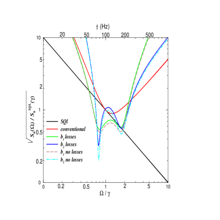
FIG. 8.: Log-log plot of $\sqrt{S_{h}(\Omega)/S_{h}^{\rm SQL}(\gamma)}$ versus $\Omega/\gamma$ for the two quadratures $b_{1}$ ($\zeta=\pi/2$)and $b_{2}$ ($\zeta=0$), including and not including losses, with $\rho=0.9$, $\phi=\pi/2-0.47$, $I_{o}=I_{\rm SQL}$, $\epsilon=0.01$, $\lambda_{\rm SR}=0.02$ and $\lambda_{\rm PD}=0.1$. The noise curve for a conventional interferometer and the SQL are shown as well.

The reason why we get a modest effect from optical losses as compared to schemes using squeezing or FD homodyne detections rests on the fact that our gain in sensitivity mostly comes from resonant amplification, which is much less susceptible to losses than quantum correlations. This general consideration has long been understood by Braginsky, Khalili and colleagues and underlies their motivation for the GW “optical bar” detectors [9].

VI Conclusions

In this paper we have extended the quantum formalism recently developed [7] for conventional interferometers (LIGO-I/TAMA/Virgo), to SR interferometer such as LIGO-II. The introduction of the SR cavity has been planned as an important tool to reshape the noise curves, making the interferometer work either in broadband or in narrowband configurations. This flexibility is expected to improve the observation of specific GW sources [17]. Quite remarkably, our quantum mechanical analysis has revealed other significant features of the SR cavity.

First, the SR mirror produces dynamical correlations between quantum shot noise and radiation-pressure-fluctuation noise which break the light’s ability to enforce the SQL of a free mass, allowing the noise curves to go below the SQL by modest amounts: roughly a factor two over a bandwidth $\Delta f\!\sim\!f$. Before our work, researchers were unaware of the shot-noise / radiation-pressure correlations and thus omitted them in their semiclassical analysis of the straw-man design of LIGO-II [21]. The goal of beating the SQL in LIGO-II can be achieved only if all sources of thermal noise can also be pushed below the SQL and indeed much R&D will go into trying to push them downward. It turns out that even with current estimates of the LIGO-II thermal noise [15], which are a little above the SQL, the net noise (thermal plus optical) is significantly affected by the shot-noise/ radiation-pressure correlations. Indeed, the correlations lift the noise at low frequencies $10\,{\rm Hz}\,\raise 1.72218pt\hbox{$<$}\kern-8.00003pt\lower 2.6694pt\hbox{$\sim$}\,\Omega/2\pi\,\raise 1.72218pt\hbox{$<$}\kern-8.00003pt\lower 2.6694pt\hbox{$\sim$}\,50$ Hz, as compared to the semiclassical estimations, even though in this frequency range the optical noise may already be very much larger than the SQL. This is due to the inaccuracy of the semiclassical method in estimating the effect of the radiation-pressure force, which is important in this region. In the middle frequency range, i.e. near 100 Hz, the SQL-beating effect cannot lower the total noise much because of the thermal contribution. The effect of the correlations in the implementation of LIGO-II will be clarified and sharpened once the readout scheme has be specified [24].

Second, we have learned that the dynamical correlations arise naturally from the nontrivial coupling between the antisymmetric mode of motion of the four arm-cavity mirrors and the signal recycled optical fields. This dynamical coupling invalidates the naive picture, according to which the arm cavity mirrors are subject only to random quantum-vacuum fluctuations. The SR interferometer responds to a GW signal as an optical spring [11], and this oscillatory response gives the possibility for resonant amplification of the GW signal. The optical-mechanical system is characterized by two resonances and one of them is always unstable, so a control system must be introduced to stabilize it [11]. In the limit of a highly reflecting SR mirror we have worked out analytically a very simple equation which locates the positions of the resonant frequencies. Whereas the amplitude of the classical output signal is amplified near the resonances, the quantum noise is not particularly affected by them. All this suggests that the beating of the SQL in SR interferometers comes primarily from the resonant amplification of the input GW signal, as also occurs in “optical bar” GW detectors [9].

The inclusion of losses does not greatly affect the SR interferometer. This is due to the fact that the improvement in the noise curves rests primarily on a resonant amplification and only modestly on ponderomotive squeezing. It is worthwhile to point out that the SR interferometers bears strong similarity to the “optical bar” detectors proposed by Braginsky, Khalili and colleagues [9]. Both of them can be viewed as oscillators with two different eigenfrequencies. However, because in SR interferometers the light plays the double role of providing the restoring force and being a probe to monitor the mirror displacements, we are forced to introduce in SR interferometers much higher laser power, to circulate in the arm cavities ($\sim\!1\,{\rm MWatt}$), than in the “optical bar” scheme. Nevertheless, like the “optical bar” scheme, the SR interferometer is still less susceptible to optical losses than many other schemes designed to beat the SQL.

It is now important to identify the best SR configuration, i.e. the choice of the physical parameters (light power $I_{o}$, SR detuning $\phi$, reflectivity of SR mirror $\rho$, quadrature phase $\zeta$, and the read-out scheme: homodyne or modulation/demodulation) that optimizes the signal-to-noise ratio for inspiraling binaries, for low-mass X-ray binaries, and for other astrophysical GW sources. We shall discuss this issue in a forthcoming paper [24].

Finally, our analysis has shown that dynamical correlations, i.e. correlations that are intrinsic to the dynamics of the test mass-optical field system (i.e. they are not due to specific read-out schemes, as in the case of homodyne detection on a conventional interferometer), are present when the carrier frequency $\omega_{o}$ is detuned from resonance ($\phi\neq 0$) or antiresonance ($\phi\neq\pi/2$) in the SR cavity. This suggests a speculation that it could be worthwhile to investigate a LIGO-II configuration (see Table I) without a signal recycling mirror, in which the correlations are produced by detuning the arm cavities. However, this case will require a very careful analysis of the radiation-pressure force acting on the arm-cavity mirrors [20], [19].

A Remark on commutation relations among quadrature fields in Caves-Schumaker two-photon formalism

As originally pointed out by Braginsky’s group [4] and discussed by BGKMTV [16], the output variables of the GW interferometer should commute with themselves at different times, to guarantee that no other quantum noise is necessarily introduced into the measurement result once further manipulations are performed on the output. Indicating generically by ${\cal O}(t)$ the output quantity, the following conditions should be satisfied,

$$[{\cal O}(t),{\cal O}(t^{\prime})]=0\quad\quad\forall\,t,t^{\prime}\,,\quad\quad\Leftrightarrow\quad\quad[{\cal O}(\Omega),{\cal O}^{\dagger}(\Omega^{\prime})]=0\quad\quad\forall\,\Omega,\Omega^{\prime}\,.$$ (A1)

If we assume that the system’s output is one quadrature of the quantized electromagnetic field (EM) [see Eq. (11)], with the GW signal encoded at side-band frequency $\Omega$ around the carrier frequency $\omega_{o}$, then the presence of terms proportional to $\Omega/\omega_{o}$ in Eq. (5) prevents the output quadratures from commuting with themselves at different times. However, Braginsky et al. [16] anticipated that, in the case of LIGO-I/TAMA/Virgo, the quadrature fields at the dark port should anyway satisfy very accurately the Fourier-domain condition given by Eq. (A1), because the side-band frequency $\Omega$ ($1\,{\rm Hz}\leq\Omega/2\pi\leq 10^{3}\,{\rm Hz}$) is much smaller than the carrier frequency $\omega_{o}$ ($\omega_{o}\!\sim\!10^{15}\,\rm s^{-1}$). In this Appendix we investigate this approximation in much more detail, estimating the amount of extra noise which will be present in the final noise spectral density as a result of condition (A1) being violated. Henceforth, for simplicity we restrict our analysis to conventional interferometers.

If the readout scheme is implemented by photodetection, then only a small frequency band around $\omega_{o}$ contains the final output signal. Hence, it is physically justified to introduce a cutoff $\Lambda$ in the frequency domain which automatically discards all the Fourier components of the EM field outside the range $\left[\omega_{o}-\Lambda,\,\omega_{o}+\Lambda\right]$ with $0\leq\Lambda\leq\omega_{o}$. As a consequence, Eq. (6) for the EM field can be rewritten as [see also Eqs. (4.22) of Ref. [22]]

$${E}^{\Lambda}(t) \equiv \int_{\omega_{o}-\Lambda}^{\omega_{o}+\Lambda}\,\sqrt{\frac{2\pi\hbar\omega}{{\cal A}c}}\,a_{\omega}\,e^{-i\omega t}\,\frac{d\omega}{2\pi}\,+\,{\rm h.c.}$$ (A2)

$$= \sqrt{\frac{2\pi\hbar\omega_{o}}{{\cal A}c}}\,e^{-i\omega_{o}t}\,\int_{0}^{\Lambda}\frac{d\Omega}{2\pi}\left({a}_{+}\,e^{-i\Omega t}+{a}_{-}\,e^{+i\Omega t}\right)\,+\,{\rm h.c.}$$ (A3)

$$= \sqrt{\frac{4\pi\hbar\omega_{o}}{{\cal A}c}}\left[\cos(\omega_{o}t)\,{{\cal O}}^{\Lambda}_{1}(t)+\sin(\omega_{o}t)\,{{\cal O}}^{\Lambda}_{2}(t)\right]\,,$$ (A4)

where $a_{+}(\Omega)$ and $a_{-}(\Omega)$, with $\Omega<\Lambda$, are defined by Eq. (3) and the rescaled quadrature fields ${{\cal O}}^{\Lambda}_{i}(t)$ are

$${{\cal O}}^{\Lambda}_{i}(t)\equiv\ \int_{0}^{\Lambda}\frac{d\Omega}{2\pi}\left[{a}_{i}\,e^{-i\Omega t}+{a}^{\dagger}_{i}\,e^{i\Omega t}\right]\quad\quad i=1,\,2\,,$$ (A5)

with the quadrature operators given by Eq. (7). Evaluating the commutation relations among the quadrature operators we find [see also Eqs. (4.31) of Ref. [22]]:

$$\left[{a}_{1},{a}_{1^{\prime}}\right]=\left[{a}_{2},{a}_{2^{\prime}}\right] = 0\,,$$ (A6)

$$\left[{a}_{1},{a}^{\dagger}_{1^{\prime}}\right]=\left[{a}_{2},{a}^{\dagger}_{2^{\prime}}\right] = 2\pi\delta(\Omega-\Omega^{\prime})\left(\frac{\Omega}{\omega_{o}}\right)\,,$$ (A7)

$$\left[{a}_{1},{a}^{\dagger}_{2^{\prime}}\right]=-\left[{a}_{2},{a}^{\dagger}_{1^{\prime}}\right] = 2\pi i\delta(\Omega-\Omega^{\prime})\,.$$ (A8)

Note that Eq. (A7) differs from the one appearing in Eq. (8), where we approximated $a_{i}$ and $a_{i^{\prime}}^{\dagger}$ as commuting. The non-vanishing commutation relations in Eq. (A7) explicitly yield a non-vanishing two-time commutator for ${{\cal O}}^{\Lambda}_{i}$. In particular, a straightforward calculation gives ($i=1,2$):

$$C_{{\cal O}_{i}^{\Lambda}{\cal O}_{i}^{\Lambda}}(t,t^{\prime})\equiv\left[{{\cal O}}^{\Lambda}_{i}(t),{{\cal O}}^{\Lambda}_{i}(t^{\prime})\right]=i\frac{\Lambda^{2}}{\omega_{o}}\left[\frac{\Lambda\tau\cos(\Lambda\tau)-\sin(\Lambda\tau)}{\pi\left(\Lambda\tau\right)^{2}}\right]\,,\quad\quad\tau=t-t^{\prime}\,.$$ (A9)

Therefore ${{\cal O}}^{\Lambda}_{i}(t)$ cannot be the final output and there must be some unavoidable additional quantum noise due to the fact that ${{\cal O}}^{\Lambda}_{i}(t)$ has a non-vanishing two-time commutator. In LIGO-I/TAMA/Virgo this additional noise is introduced in the output during the final process of photodetection. A more detailed study would involve a very technical analysis of the photodetection’s dynamics, but fortunately, as we shall see in the following, a simple estimation of the order of magnitude of this additional quantum noise suggests that it is very small and we can realistically neglect it.

We find it convenient to estimate the additional quantum noise by calculating the noise induced by the photodetector approximated as a linear measurement device coupled to the quadrature fields. Having fixed the cutoff frequency $\Lambda$ and working in the Fourier domain, we can write the final output as:

$${{\cal O}}^{out}_{i}(\Omega)={{\cal O}}^{\Lambda}_{i}(\Omega)+{Z}^{{\rm PD}}_{i}(\Omega)+R_{{\cal O}_{i}^{\Lambda}{\cal O}_{i}^{\Lambda}}(\Omega)\,{F}^{{\rm PD}}_{i}(\Omega)\,,$$ (A10)

where

$$R_{{\cal O}_{i}^{\Lambda}{\cal O}_{i}^{\Lambda}}(\Omega)\equiv\frac{i}{\hbar}\int_{0}^{+\infty}d\tau\,e^{i\Omega\tau}\,C_{{\cal O}_{i}^{\Lambda}{\cal O}_{i}^{\Lambda}}(t,t-\tau)=\frac{1}{2\pi\hbar\omega_{o}}\left(2\Lambda+i\pi\Omega+\Omega\ln\frac{\Lambda-\Omega}{\Lambda+\Omega}\right)\,.$$ (A11)

The last two terms in Eq. (A10) are the shot noise and the back-action noise of the photodetector (PD) and describe the efficiency and the strength of perturbation of the PD on the quadrature field, respectively. Let us assume that there is no correlation between ${Z}^{{\rm PD}}_{i}$ and ${F}^{{\rm PD}}_{i}$. Hence, ${Z}^{{\rm PD}}_{i}$ and ${F}^{{\rm PD}}_{i}$ satisfy the uncorrelated version (48) of the uncertainty relation, that is

$$S_{{Z}_{i}^{{\rm PD}}{Z}_{i}^{{\rm PD}}}S_{{F}_{i}^{{\rm PD}}{F}_{i}^{{\rm PD}}}\geq\hbar^{2}\,.$$ (A12)

We are interested in evaluating the overall quantum noise. We first write the output in the form Signal + Noise as

$${{\cal O}}^{\rm out}_{i}(\Omega)={\cal{P}}_{i}h(\Omega)+\left[{\cal Q}^{\Lambda}_{i}(\Omega)+{Z}^{{\rm PD}}_{i}(\Omega)+R_{{\cal O}_{i}^{\Lambda}{\cal O}^{\Lambda}_{i}}(\Omega){F}^{{\rm PD}}_{i}(\Omega)\right]\,,$$ (A13)

where ${\cal{P}}_{i}h$ is the part of ${{\cal O}}^{\Lambda}_{i}(\Omega)$ that contains the signal, while ${\cal Q}^{\Lambda}_{i}(\Omega)$ contains the quantum fluctuations. Using Eq. (A13), the overall noise spectral density is ($i=1,2$):

$$S_{i}(\Omega)=\frac{1}{\left|{\cal P}_{i}\right|^{2}}\left\{S_{{\cal Q}_{i}^{\Lambda}{\cal Q}_{i}^{\Lambda}}(\Omega)+S_{{Z}_{i}^{{\rm PD}}{Z}_{i}^{{\rm PD}}}(\Omega)+\left|R_{{\cal O}_{i}^{\Lambda}{\cal O}^{\Lambda}_{i}}(\Omega)\right|^{2}S_{{F}_{i}^{{\rm PD}}{F}_{i}^{{\rm PD}}}(\Omega)\right\}\,.$$ (A14)

The first term in Eq. (A14) describes the quantum noise of an interferometer when the non-vanishing commutators of the quadrature fields have been ignored and ideal photodetection is applied. The second term in Eq. (A14) describes the additional shot noise introduced by the photodetection process. Finally, the third term comes from the back-action force acting on the measured quadrature ($i=1$ or $2$) because it does not commute with itself at different times. Let us notice that, given Eq. (A12), the second and third noise contributions appearing on the RHS of Eq. (A14) are complementary. Indeed, the larger the shot noise, the weaker the minimum force the photodetector must apply to the quadrature fields and the smaller the back-action noise. More specifically, there is a lowest achievable value for the PD part in Eq. (A14) given by:

$$\frac{1}{|{\cal P}_{i}|^{2}}\left[S_{{Z}_{i}^{{\rm PD}}{Z}_{i}^{{\rm PD}}}(\Omega)+\left|R_{{\cal O}^{\Lambda}_{i}{\cal O}^{\Lambda}_{i}}(\Omega)\right|^{2}S_{{F}_{i}^{{\rm PD}}{F}_{i}^{{\rm PD}}}(\Omega)\right] \geq \frac{2|R_{{\cal O}^{\Lambda}_{i}{\cal O}^{\Lambda}_{i}}(\Omega)|\hbar}{|{\cal P}_{i}|^{2}}\,,$$ (A15)

$$= \frac{2}{|{\cal P}_{i}|^{2}}\left|\frac{\Lambda}{\pi\omega_{o}}\left(1+\frac{\Omega}{2\Lambda}\ln\frac{\Lambda-\Omega}{\Lambda+\Omega}\right)+i\frac{\Omega}{\omega_{o}}\right|\,.$$ (A16)

Using Eq. (40) we derive ${1}/{|{\cal S}_{i}|^{2}}={h_{\rm SQL}^{2}}/{2\cal K}$ and $S_{{\cal Q}_{i}^{\Lambda}{\cal Q}_{i}^{\Lambda}}=({\cal K}^{2}+1)>1$. Recalling that $10\,{\rm Hz}\leq\Omega/2\pi\leq 10^{3}\,{\rm Hz}$ and $\omega_{o}\!\sim\!10^{15}\,{\rm sec}^{-1}$, fixing $\Lambda$ to a value larger than the typical $\Omega$, e.g., $\Lambda/2\pi\!\sim\!10\,{\rm MHz}$, and adjusting the PD such that $S_{{Z}_{i}^{{\rm PD}}{Z}_{i}^{{\rm PD}}}$ and $S_{{F}_{i}^{{\rm PD}}{F}_{i}^{{\rm PD}}}$ satisfy the minimal uncertainty relation [the equality sign in Eq. (A12)], we find that the minimal achievable PD noise is $\sim\!10^{-7}$ times the conventional shot noise. Therefore, we can totally ignore the quantum noise introduced by the fact that the quadrature fields do not commute with themselves at different times in Eq. (A7). Note the importance of the cutoff $\Lambda$. If we had taken $\Lambda\!\sim\!\omega_{o}$, the limit on the PD noise would have been of the same order of magnitude as the shot noise for a conventional interferometer and it would not have been realistic to neglect the quantum noise introduced by the non-vanishing commutation relations of the quadrature fields.

So far we evaluated the minimum quantum noise that the photodetector, coupled linearly to the quadrature field, can introduce. Let us now try to give a realistic value of it. To estimate $S_{{Z}_{i}^{{\rm PD}}{Z}_{i}^{{\rm PD}}}$, we can just recall that in the case of a lossy photodetector we have (see the discussion of lossy interferometers in Sec. V)

$${Z}^{{\rm PD}}_{i}\!\sim\!\sqrt{\lambda_{{\rm PD}}}\,{p}_{i}\,,$$ (A17)

where $p_{i}$ with $i=1,2$ are quadrature operators in the vacuum state. We expect $\lambda_{{\rm PD}}\!\sim\!0.1-0.2$, hence $S_{{Z}_{i}^{{\rm PD}}{Z}_{i}^{{\rm PD}}}>10^{-2}\times S_{\rm shot\,noise}^{\rm conv}$, which is five orders of magnitude larger than the lowest achievable limit discussed above with $\Lambda/2\pi\!\sim\!10\,{\rm MHz}$. Therefore, if one can justify fixing the cutoff $\Lambda/2\pi$ at $10\,{\rm MHz}$, and if the uncertainty relation (A12) is satisfied with the equality sign, then one can conclude that the inefficiency will dominate over the minimum possible back-action noise by five orders of magnitude. Hence, we are justified in disregarding the non-vanishing two-time commutators of the quadrature fields in Eq. (A7).

REFERENCES

- [1] A. Abramovici et al., Science 256 (1992) 325; C. Bradaschia et al., Nucl. Instrum. Meth. A 289 (1990) 518; K. Danzmann et al., in First Edoardo Amaldi Conference on Gravitational Wave Experiments, Frascati 1994 (World Scientific, Singapore, 1995); K. Tsubono, in First Edoardo Amaldi Conference on Gravitational Wave Experiments, Frascati 1994 (World Scientific, Singapore, 1995).
- [2] See, e.g., Secs. 9.5.2 and 9.5.3 of K.S. Thorne, in Three Hundred Years of Gravitation, eds. S.W. Hawking and W. Israel, (Cambridge University Press, Cambridge, 1987), and references therein.
- [3] V.B. Braginsky, Sov. Phys. JETP 26 (1968) 831; V.B. Braginsky and Yu.I. Vorontsov, Sov. Phys. Uspekhi 17 (1975) 644; V.B. Braginsky, Yu.I. Vorontsov and F.Ya. Kahili, Sov. Phys. JETP 46 (1977) 705.
- [4] V.B. Braginsky and F.Ya. Khalili, Quantum measurement, ed. K.S. Thorne (Cambridge University Press, Cambridge, 1992).
- [5] See, e.g., Appendix B of V.B. Braginsky, M.L. Gorodetsky, F.Ya. Khalili and K.S. Thorne, Phys. Rev. D61 (2000) 044002 [gr-qc/9906108]; P. Purdue, in preparation.
- [6] C.M. Caves, Phys. Rev. D 23 (1981) 1693; W.G. Unruh, in Quantum Optics, Experimental Gravitation, and Measurement Theory, eds. P. Meystre and M.O. Scully (Plenum, 1982), p. 647; M.T. Jaekel and S. Reynaud, Europhys. Lett. 13 (1990) 301.
- [7] H.J. Kimble, Yu. Levin, A.B. Matsko, K.S. Thorne and S.P. Vyatchanin, Conversion of conventional gravitational-wave interferometers into QND interferometers by modifying input and/or output optics, submitted to Phys. Rev. D [gr-qc/0008026]. It is referred to as KLMTV in this paper.
- [8] S.P. Vyatchanin and A.B. Matsko, JETP 77 (1993) 218; S.P. Vyatchanin and E.A. Zubova, Phys. Lett. A 203 (1995) 269; S.P. Vyatchanin and A.B. Matsko, JETP 82 (1996) 1007; ibid. JETP 83 (1996) 690; S.P. Vyatchanin, Phys. Lett. A 239 (1998) 201.
- [9] V.B. Braginsky, M.L. Gorodetsky and F.Ya. Khalili, Phys. Lett. A 232 (1997) 340; V.B. Braginsky and F.Ya. Khalili, Phys. Lett. A 257 (1999) 241.
- [10] H.P. Yuen, Phys. Rev. Lett. 51 (1983) 719; C.M. Caves, Phys. Rev. Lett. 54 (1985) 2465; M. Ozawa, Phys. Rev. Lett. 60 (1988) 385; Phys. Rev. A 41 (1990) 1735; J. Maddox, Nature 331 (1988) 559.
- [11] A. Buonanno and Y. Chen, Signal recycled laser-interferometer gravitational-wave detectors as optical springs, GRP/00/554, submitted to Phys. Rev. D, [gr-qc/0107021].
- [12] A. Buonanno and Y. Chen, Optical noise correlations and beating the standard quantum limit in advanced gravitational-wave detectors, GRP/00/549, accepted for publication in Class. Quantum Grav., [gr-qc/0010011].
- [13] B.J. Meers, Phys. Rev. D 38 (1988) 2317; J.Y. Vinet, B. Meers, C.N. Man and A. Brillet, Phys. Rev. D 38 (1988) 433.
- [14] J. Mizuno, Comparison of optical configurations for laser interferometric gravitatioanl-wave detectors, PhD thesis (1995); J. Mizuno, K.A. Strain, P.G. Nelson, J.M. Chen, R. Schilling, A. Rüdiger, W. Winkler and K. Danzmann, Phys. Lett. A 175 (1993) 273.
- [15] V.B. Braginsky, M.L. Gorodetsky and S.P. Vyatchanin, Phys. Lett. A 264 (1999) 1; Y.T. Liu and K.S. Thorne, Phys. Rev. D 62 (2000) 122002; V.B. Braginsky, E. D’Ambrosio, R. O’Shaughnessy, S.E. Strigen, K.S. Thorne and S.P. Vyatchanin, in preparation.
- [16] V.B. Braginsky, M.L. Gorodetsky, F.Ya. Khalili, A.B. Matsko, K.S. Thorne and S.P. Vyatchanin, Noise in gravitational-wave detectors is not influenced by test-mass quantization, in preparation. It is referred to as BGKMTV in this paper.
- [17] See, e.g., A. Abramovici et al. in Ref. [1]; K.S. Thorne, in Proceedings of the Snowmass 95 Summer Study on Particle and Nuclear Astrophysics and Cosmology, eds. E.W. Kolb and R. Peccei (World Scientific, Singapore, 1995), p. 398 [gr-qc/9506085]; K.S. Thorne, The scientific case for advanced LIGO interferometers, LIGO Document Number P-000024-00-D.
- [18] A. Dorsel, J.D. McCullen, P. Meystre, E. Vignes and H. Walther, Phys. Rev. Lett. 51 (1983) 1550; N. Deruelle and P. Tourrenc, in Gravitation, Geometry and Relativistic Physics (Springer, Berlin, 1984); P. Meystre, E.M. Wright, J.D. McCullen and E. Vignes, J. Opt. Soc. Am. 2 (1985) 1830; J.M. Aguirregabria and L. Bel, Phys. Rev. D 36 (1987) 3768; L. Bel, J.L. Boulanger and N. Deruelle, Phys. Rev. A 7 (1988) 37.
- [19] G. Heinzel, Advanced optical techniques for laser interferometric gravitational-wave detectors, PhD thesis (1999); M. Rachmanov, Dynamics of laser interferometric gravitational wave detectors, PhD thesis (2000).
- [20] A. Pai, S.V. Dhurandhar, P. Hello and J-Y. Vinet, Euro. Phys. J. D 8 (2000) 333.
- [21] E. Gustafson, D. Shoemaker, K. Strain and R. Weiss, LSC White paper on Detector Research and Development, LIGO Document Number T990080-00-D (Caltech/MIT, 11 September 1999). See also www.ligo.caltech.edu/ligo2/.
- [22] C.M. Caves and B.L. Schumaker, Phys. Rev. A 31 (1985) 3068.
- [23] B.L. Schumaker and C.M. Caves, Phys. Rev. A 31 (1985) 3093.
- [24] A. Buonanno and Y. Chen, in preparation.
- [25] See, e.g., R.C. Dorf, Modern Control Systems, (Addison-Wesley, Reading Massachusetts, 1990), Chap. 7 and 8.
- [26] See, e.g., S. Ichimaru, Basic Principles of Plasma Physics, (Benjamin, Reading Massachusetts 1973).
- [27] See, e.g., J. Mathews and R.L. Walker, Mathematical Methods of Physics, (Addison-Wesley, Reading Massachusetts, 1970).
- [28] K. Strain, private communication.
- [29] R. Drever, in Gravitational Radiation, ed. N. Deruelle and T. Piran (North-Holland, Amsterdam, 1983), pp. 321-338.
- [30] A. Freise, G. Heinzel, K.A. Strain, J. Mizuno, K.D. Skeldon, H. Lück, B. Wilke, R. Schilling, A. Rüdiger, W. Wingler and K. Danzmann, Phys. Lett. A277 (2000) 135 [gr-qc/0006026].
- [31] J. Mason, Signal Extraction and Optical Design for an Advanced Gravitational Wave Interferometer, PhD thesis, (2001). [LIGO document P010010-00-R, www.ligo.caltech.edu/docs/P/P010010-00.pdf]