Abstract

We compute the spectral distribution of the quantum fluctuations of the vacuum, amplified by inflation, after an arbitrary number of background transitions. Using a graphic representation of the process we find that the final spectrum can be completely determined trough a synthetic set of working rules, and a list of simple algebraic computations.

A diagrammatic approach to the spectrum
of cosmological perturbations

G. De Risi and M. Gasperini

Dipartimento di Fisica, Università di Bari,
Via G. Amendola 173, 70126 Bari, Italy
and
Istituto Nazionale di Fisica Nucleare, Sezione di Bari, Bari, Italy

The standard cosmological model [2], in spite of the large number of successful predictions, cannot be extrapolated too far back in time. It is by now a consolitated opinion that our Universe, in its earlier epochs, should include a phase of inflationary (i.e. accelerated) evolution [3]. Many different realizations of inflation are possible, however, and we have to face the problem of how to distinguish them through their possible phenomenological consequences.

To this aim, we may note that the instability of the small fluctuations (of the metric and of the matter fields) is one of the main physical properties of a phase of accelerated evolution. As a consequence of this instability, small perturbations are amplified in a way which depends on the intensity and on the duration of inflation [4]. Different inflationary models amplify perturbations with different spectral distribution, and the computation of the spectrum thus becomes an important tool to predict observable effects, and to discriminate eventually between various possible models of primordial evolution.

The computation of the spectrum, performed accorting to the standard cosmological perturbation theory [4], may become long and cumbersome even in the linear approximation, however, if the model of cosmological background is complicated. The aim of this paper is to present a set of working rules, based on a diagrammatic representation of the evolution of perturbations, allowing a quick estimate of the final amplitude and of the spectral distribution. The idea of a diagrammatic approach is not new [5], but it was never implemented up to now in a complete and systematic way, so as to be generally valid for all classes of inflationary backgrounds.

To be more precise, the diagrammatic method of computation that we shall propose here can be applied to all cosmological fluctuations $\psi$ described by the quadratic effective action

$$S={1\over 2}\int d\eta~{}z^{2}(\eta)\left(\psi^{\prime 2}+\psi\nabla^{2}\psi\right),$$ (1)

where $z$ is the external “pump field”, responsible for the amplification, and the prime denotes differentiation with respect to the conformal time $\eta$. It is convenient, in this context, to introduce the canonical variable $u=z\psi$ which diagonalizes the effective action, and which satisfies the canonical evolution equation [4]

$$u^{{}^{\prime\prime}}_{k}+\left(k^{2}-{z^{\prime\prime}\over z}\right)u_{k}=0$$ (2)

(for each mode $k$ of the Fourier expansion, $\nabla^{2}u_{k}=-k^{2}u_{k}$). We shall also assume that the background evolution can be separated into $n+1$ different cosmological phases, with $n$ transitions at $\eta=\eta_{i}$, $i=1,...,n$, and that in each phase the evolution of the pump fields (sufficiently far from the transition) can be parametrized in conformal time by an appropriate power $\alpha_{i}$, namely $z_{i}\sim|\eta|^{\alpha_{i}}$. It follows that, in each phase, the general solution of eq. (2) can be written in terms of the first and second kind Hankel functions [6] as:

$$u^{i}_{k}(\eta)=|\eta|^{1\over 2}\left[A^{i}_{+}(k)H^{(1)}_{\mu_{i}}(x)+A^{i}_{-}(k)H^{(2)}_{\mu_{i}}(x)\right],~{}~{}~{}~{}~{}\mu_{i}=|\alpha_{i}-{1/2}|,~{}~{}~{}~{}~{}x=k|\eta|.$$ (3)

In order to fix our conventions, we shall label the $n$ transitions in decreasing order for $\eta$ ranging from $-\infty$ to $+\infty$, and we shall put the power $\alpha_{i}$ to the right (and $\alpha_{i+1}$ to the left) of $\eta_{i}$, namely

$$z_{i+1}\sim|\eta|^{\alpha_{i+1}},~{}~{}~{}~{}\eta<\eta_{i},~{}~{}~{}~{}~{}~{}~{}~{}~{}~{}~{}~{}~{}~{}z_{i}\sim|\eta|^{\alpha_{i}},~{}~{}~{}~{}\eta>\eta_{i}$$ (4)

It follows that the first (in order of time) cosmological phase is labelled by $n+1$, the last one by $1$. The normalization to an initial vacuum fluctuation spectrum [4] thus imposes $A_{+}^{n+1}=1$, $A_{-}^{n+1}=0$, while the coefficients of the last phase $A^{1}_{\pm}(k)$, fixed by the continuity of $\psi_{k}$ and $\psi^{\prime}_{k}$ at the transitions $\eta_{i}$ (not of $u_{k}$ and $u^{\prime}_{k}$, see the discussion in [7]), will determine the final spectral distribution of the amplified perturbations. The spectral energy density, in particular, is given by [4] $d\rho/d\log k=(k/a)^{4}|A^{1}_{-}(k)|^{2}/\pi^{2}$ or, in critical units and in terms of the proper frequency $\omega=k/a$,

$$\Omega(\omega,t)={8\over 3\pi}{\omega^{4}\over M^{2}_{p}H^{2}}|A^{1}_{-}(\omega)|^{2}.$$ (5)

The computation of the spectrum thus reduces, in general, to the problem of solving a linear non-omogeneous system of $2n$ equations,

$$\psi_{k}^{i+1}(x_{i})=\psi_{k}^{i}(x_{i}),~{}~{}~{}~{}~{}~{}~{}~{}~{}~{}~{}~{}\psi_{k}^{\prime~{}i+1}(x_{i})=\psi_{k}^{\prime~{}i}(x_{i}),$$ (6)

for the $2n$ unknown quantities $A^{i}_{\pm}(k)$. The solution is straightforward, in principle; in practice, however, it is in general arduous to extract the relevant physical information from the exact solution, for any background with $n\geq 2$. In this paper we shall derive a set of prescriptions enabling an immediate estimate of the spectral coefficient $A^{1}_{-}(k)$, through an approximate procedure which captures the essential features (amplitude and frequency dependence) of the spectrum, without solving explicitly the full system of equations. Such an estimate is based on the asymptotic expansion of the Hankel functions, and on the possible separation of the spectrum into $n$ frequency bands, depending on the number of transitions which are truly effective for a given frequency mode.

In order to introduce the basic ideas of our procedure, we shall start considering the simplest case of only one transition at $\eta=\eta_{1}$. The normalized solution of eq. (2) is then

$$u^{1}_{k}=|\eta|^{{1\over 2}}H^{(1)}_{\mu_{1}}(x),$$ (7)

$$u^{2}_{k}=|\eta|^{{1\over 2}}\left[A^{1}_{+}H^{(1)}_{\mu_{2}}(x)+A^{1}_{-}H^{(2)}_{\mu_{2}}(x)\right]$$ (8)

(with $\mu_{1}\neq\mu_{2}$), and the continuity of $\psi_{k}$ at $\eta_{1}$ provides for the spectral coefficients the following exact solution [7]:

$$A^{1}_{-}={i\pi\over 4}\left[x_{1}\left(H^{{}^{\prime}(1)}_{\mu_{2}}H^{(1)}_{\mu_{1}}-H^{(1)}_{\mu_{2}}H^{{}^{\prime}(1)}_{\mu_{1}}\right)+\left(\alpha_{1}-\alpha_{2}\right)H^{(1)}_{\mu_{2}}H^{(1)}_{\mu_{1}}\right],$$ (9)

$$A^{1}_{+}={i\pi\over 4}\left[x_{1}\left(H^{(1)}_{\mu_{2}}H^{{}^{\prime}(2)}_{\mu_{1}}-H^{{}^{\prime}(1)}_{\mu_{2}}H^{(2)}_{\mu_{1}}\right)+\left(\alpha_{2}-\alpha_{1}\right)H^{(1)}_{\mu_{2}}H^{(2)}_{\mu_{1}}\right],$$ (10)

where the Hankel functions are evaluated ay $x_{1}=k|\eta_{1}|$. These coefficients satisfy the canonical normalization $|A_{+}|^{2}-|A_{-}|^{2}=1$.

The time scale $\eta_{1}$ defines the typical transition frequency, $k_{1}=|\eta_{1}|^{-1}$. For modes with $k\gg k_{1}$ we can use the large argument limit of the Hankel functions, and we obtain $A^{1}_{-}\simeq 0$, $A^{1}_{+}\simeq 1$: such modes are thus unaffected by the transition, modulo higher order corrections that are esponentially damped like $e^{-k/k_{1}}$ (see [8], for instance), and that we shall neglect in our approximation. For low frequency modes, $k\ll k_{1}$, we can use instead the small argument limit [6],

$$H^{(1)}_{\mu}(x)\simeq p_{\mu}x^{\mu}+iq_{\mu}x^{-\mu}-ir_{\mu}x^{2-\mu}+s_{\mu}x^{2+\mu}+...,~{}~{}~{}~{}~{}~{}~{}~{}~{}x\rightarrow 0$$ (11)

$$H^{(2)}_{\mu}(x)\simeq p_{\mu}^{*}x^{\mu}-iq_{\mu}x^{-\mu}+ir_{\mu}x^{2-\mu}+s_{\mu}^{*}x^{2+\mu}+...,~{}~{}~{}~{}~{}~{}~{}~{}~{}x\rightarrow 0$$ (12)

where the coefficients $p,q,...$ are complex numbers with modulo of order one (for later use, we have also included higher order corrections). The exact solution (10) provides, in this limit,

$$A^{1}_{-}\simeq C^{1}_{1}x_{1}^{-\mu_{2}-\mu_{1}}+C^{1}_{2}x_{1}^{-\mu_{2}+\mu_{1}}+C^{1}_{3}x_{1}^{\mu_{2}-\mu_{1}}+C^{1}_{4}x_{1}^{2-\mu_{2}-\mu_{1}}+...$$ (13)

where

$$C^{1}_{1}={i\pi\over 4}q_{\mu_{1}}q_{\mu_{2}}\left(\mu_{2}-\mu_{1}+\alpha_{2}-\alpha_{1}\right),$$ (14)

$$C^{1}_{2}=-{\pi\over 4}p_{\mu_{1}}q_{\mu_{2}}\left(-\mu_{2}-\mu_{1}-\alpha_{2}+\alpha_{1}\right),$$ (15)

$$C^{1}_{3}=-{\pi\over 4}q_{\mu_{1}}p_{\mu_{2}}\left(\mu_{2}+\mu_{1}-\alpha_{2}+\alpha_{1}\right),$$ (16)

$$C^{1}_{4}={i\pi\over 4}\left[q_{\mu_{1}}r_{\mu_{2}}\left(2-\mu_{2}+\mu_{1}-\alpha_{2}+\alpha_{1}\right)+r_{\mu_{1}}q_{\mu_{2}}\left(-2-\mu_{2}+\mu_{1}-\alpha_{2}+\alpha_{1}\right)\right]$$ (17)

(and a similar expression for $A^{1}_{-}$).

By recalling that $\mu_{i}=|\alpha_{i}-1/2|$, it follows that the first term of the expansion (13) is the leading one, for $x_{1}\rightarrow 0$. When $C^{1}_{1}=0$, however, we have to include the next-to-leading corrections. Taking into account all possible values of $\alpha_{1}$, $\alpha_{2}$, and truncating the expansion (13) to the lowest order term with non-vanishing coefficients, we find that for $\alpha_{1}\neq\alpha_{2}$ there are four different possibilities, corresponding to four different spectral amplitudes:

$$\alpha_{2}>1/2~{}{\rm or}~{}\alpha_{1}>1/2,~{}~{}~{}~{}~{}~{}~{}~{}~{}~{} A^{1}_{-}\simeq C^{1}_{1}x_{1}^{-\mu_{2}}x_{1}^{-\mu_{1}},$$ (18)

$$\alpha_{1}>-1/2,~{}\alpha_{1}>\alpha_{2},~{}~{}~{}~{}~{}~{}~{}~{}~{}~{} A^{1}_{-}\simeq C^{1}_{2}x_{1}^{-\mu_{2}}x_{1}^{\mu_{1}},$$ (19)

$$\alpha_{2}>-1/2,~{}\alpha_{2}>\alpha_{1},~{}~{}~{}~{}~{}~{}~{}~{}~{}~{} A^{1}_{-}\simeq C^{1}_{3}x_{1}^{\mu_{2}}x_{1}^{-\mu_{1}},$$ (20)

$$\alpha_{2}\leq-1/2,\alpha_{1}\leq-1/2,~{}~{}~{}~{}~{}~{}~{}~{}~{}~{} A^{1}_{-}\simeq C^{1}_{4}x_{1}^{-\mu_{2}+1}x_{1}^{-\mu_{1}+1},$$ (21)

in agreement with the results first obtained in [7].

If one of the two powers $\alpha_{1}$, $\alpha_{2}$ equals $1/2$, the corresponding Bessel index is $\mu=0$, and the small argument expansion (12) is to be replaced by

$$H^{(1)}_{0}(x)\simeq p_{0}+iq_{0}\log x-ir_{0}x^{2}\log x+s_{0}x^{2}+...,~{}~{}~{}~{}~{}~{}~{}x\rightarrow 0,$$ (22)

$$H^{(2)}_{0}(x)\simeq p_{0}^{*}-iq_{0}\log x+ir_{0}x^{2}\log x+s_{0}^{*}x^{2}+...,~{}~{}~{}~{}~{}~{}~{}x\rightarrow 0.$$ (23)

Suppose, for instance, that $\alpha_{1}=1/2$. The exact solution (10) is now approximated by

$$A^{1}_{-}\simeq C^{1}_{1}x_{1}^{-\mu_{2}}\log x_{1}+\overline{C}^{1}_{2}x_{1}^{-\mu_{2}}+...,$$ (24)

where

$$\overline{C}^{1}_{2}=-\frac{\pi}{4}\left[q_{\mu_{2}}p_{0}\left(-\mu_{2}-\alpha_{2}+{1\over 2}\right)-iq_{\mu_{2}}q_{0}\right].$$ (25)

As $\overline{C}^{1}_{1}$ is always nonzero, the leading term in eq. (24) is the firs one for $\alpha_{2}>1/2$, and the second one for $\alpha_{2}<1/2$. We may thus include also the value $\alpha=1/2$ in the general rules (21), provided we take into account the prescription

$$x^{-\mu}|_{\mu=0}\rightarrow\log x,~{}~{}~{}~{}~{}~{}~{}~{}x^{\mu}|_{\mu=0}\rightarrow 1.$$ (26)

The above computation for a single background transition can be easily iterated for a cosmological model containing two or more transitions. We have solved the general case with $n$ transitions, and we have found the remarkable result that the vanishing of the leading term of the asymptotic expansion - and then the particular spectral behaviour of the solution - depends only on the kinematic powers $\alpha_{i}$ of two phases: the one preceding the first transition, and the one following the last transition. Such a result is in agreement with the well known phenomenon of “freezing” of perturbations [4], and with the general duality properties [9] of the action (1).

Using the above result, it becomes possible to write down a recurrent expansion for the spectrum after $n$ transition. To this aim, it is convenient to represent the whole amplification process with a simple diagram, in which we insert a vertical line in correspondence of each transition. The height of the i-th line is proportional to the associated transition frequency, $k_{i}=|\eta_{i}|^{-1}$. It become possible, in this way, to identify at a glance the various frequency bands ($k$) of the spectrum, according to the number of transitions (with $k_{i}>k$) from which a given band is significatively affected. Note that, for $\eta$ growing from minus infinity, the height of the vertical lines may grow monothonically up to a maximum transition frequency (corresponding to a minimum time scale), and is then monothonically decreasing for $\eta$ running towards plus infinity.

Let us start with the case in which the transition frequencies $k_{i}=|\eta_{i}|^{-1}$ are arranged in growing order from the left to the right (see Fig. 1). The frequency band with $k>k_{1}$ is not amplified and we shall disregard it. The band number $1$ of the diagram ($k_{2}<k<k_{1}$) will be affected by one transition, the band number $2$ ($k_{3}<k<k_{2}$) by two transitions, and so on. The iteration of the matching procedure used for a single transition leads to a recurrent expression for the coefficient $A_{-}$, where the $k$-dependence is fixed by the first and last phase, and the amplitude is fixed by the continuity at the transitions. We can write, in particular,

$$|A^{1}_{-}(k)| \simeq x_{1}^{\gamma_{21}}x_{1}^{\gamma_{12}},~{}~{}~{}~{}~{}~{}~{}~{}~{}~{}~{}~{}~{}~{}~{}~{}~{}~{}~{}~{}~{}~{}~{}~{}~{}~{}~{}~{}~{}~{}~{}~{}~{}~{}~{}~{}~{}~{}~{}~{}~{}~{}~{}~{}~{}~{}~{}~{}~{}~{}~{}~{}~{}~{}~{}~{}~{}~{}~{}~{}k_{2}<k<k_{1}$$ (27)

$$\simeq x_{2}^{\gamma_{31}}x_{1}^{\gamma_{13}}\left(\frac{x_{1}}{x_{2}}\right)^{\gamma_{21}}\left(\frac{x_{1}}{x_{2}}\right)^{\gamma_{12}-\gamma_{13}},~{}~{}~{}~{}~{}~{}~{}~{}~{}~{}~{}~{}~{}~{}~{}~{}~{}~{}~{}~{}~{}~{}~{}~{}~{}~{}~{}~{}~{}~{}~{}~{}~{}k_{3}<k<k_{2}$$ (28)

$$\vdots$$ (29)

$$\simeq x_{n}^{\gamma_{n+1,1}}x_{1}^{\gamma_{1,n+1}}\left(\frac{x_{n-1}}{x_{n}}\right)^{\gamma_{n1}}\left(\frac{x_{1}}{x_{n}}\right)^{\gamma_{1n}-\gamma_{1,n+1}}...$$ (31)

$$...\left(\frac{x_{i-1}}{x_{i}}\right)^{\gamma_{i1}}\left(\frac{x_{1}}{x_{i}}\right)^{\gamma_{1i}-\gamma_{1,i+1}}...\left(\frac{x_{1}}{x_{2}}\right)^{\gamma_{21}}\left(\frac{x_{1}}{x_{2}}\right)^{\gamma_{12}-\gamma_{13}},~{}~{}~{}~{}~{}~{}k<k_{n}$$

(modulo a numerical factor of order one, that can be computed from the exact solution, but that we shall neglect for our purpose of a quick approximate estimate).

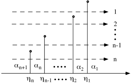
FIG. 1.: The $n$ frequency bands of the spectrum for a background with $n$ transition frequencies, arranged in growing order.

The powers $\gamma_{ik}$ of eq. (31) depend (in ordered way) on $\alpha_{i},\alpha_{k}$ according to the same rules of eq. (21), with the only difference that when $\alpha_{i}$ and $\alpha_{k}$ are not contiguous (i.e., $\alpha_{i}\not=\alpha_{k+1}$), they can also have the same value. In that case $\mu_{i}=\mu_{k}$, and the lowest order non-vanishing term of the expansion leads to $x_{i-1}^{-\mu_{i}}x_{k}^{\mu_{i}}$ if $x_{i-1}<x_{k}$, or to $x_{i-1}^{\mu_{i}}x_{k}^{-\mu_{i}}$ if $x_{i-1}>x_{k}$ (see eq. (17), where $C_{2}^{1}=-C_{3}^{1}\not=0$ for $\mu_{1}=\mu_{2}$). By summarizing the working rules for computing the powers $\gamma_{ik}$ we must then distinguish two cases. In the case $\alpha_{i}=\alpha_{k}$ we have:

$$\alpha_{i}=\alpha_{k},~{}~{}~{}\Rightarrow~{}~{}~{} \gamma_{ik}=\epsilon_{ik}\mu_{i},~{}~{}~{}~{}~{}~{}~{}~{}~{}\gamma_{ki}=-\epsilon_{ik}\mu_{i},$$ (33)

$$\epsilon_{ik}={\rm sign}\log\left(x_{i-1}\over x_{k}\right)={\rm sign}\log\left(k_{k}\over k_{i-1}\right).$$

Otherwise ($\alpha_{i}\not=\alpha_{k}$) we have, according to eq. (21):

$$\alpha_{i}>1/2~{}{\rm or}~{}\alpha_{k}>1/2,~{}~{}~{}~{}\Rightarrow~{}~{}~{}~{} \gamma_{ik}=-\mu_{i},~{}~{}~{}~{}~{}~{}~{}~{}~{}~{}~{}~{}~{}\gamma_{ki}=-\mu_{k},$$ (34)

$$\alpha_{i}>-1/2,~{}\alpha_{i}>\alpha_{k},~{}~{}~{}~{}~{}~{}\Rightarrow~{}~{}~{}~{} \gamma_{ik}=\mu_{i},~{}~{}~{}~{}~{}~{}~{}~{}~{}~{}~{}~{}~{}~{}~{}\gamma_{ki}=-\mu_{k},$$ (35)

$$\alpha_{k}>-1/2,~{}\alpha_{k}>\alpha_{i},~{}~{}~{}~{}~{}~{}\Rightarrow~{}~{}~{}~{} \gamma_{ik}=-\mu_{i},~{}~{}~{}~{}~{}~{}~{}~{}~{}~{}~{}~{}\gamma_{ki}=\mu_{k},$$ (36)

$$\alpha_{i}\leq-1/2,\alpha_{k}\leq-1/2,~{}~{}~{}~{}\Rightarrow~{}~{}~{}~{} \gamma_{ik}=-\mu_{i}+1,~{}~{}~{}~{}~{}~{}~{}\gamma_{ki}=-\mu_{k}+1,$$ (37)

Note that $\gamma_{ik}\not=\gamma_{ki}$, but that $\gamma_{ik}(\alpha_{i},\alpha_{k})=\gamma_{ik}(\alpha_{k},\alpha_{i})$. Note also that, in the limiting case in which $\mu_{i}=0$ or $\mu_{k}=0$, we can take into account the logarithmic corrections according to the prescription (26). However, as they are usually negligible in realistic models, we shall neglect the log corrections in our first estimate of the spectrum, using the simple rule:

$$\gamma_{ik}\left({1\over 2},\alpha_{k}\right)=0,~{}~{}~{}~{}~{}~{}~{}~{}~{}~{}~{}~{}~{}~{}~{}~{}\gamma_{ki}\left({1\over 2},\alpha_{k}\right)=-\mu_{k}=\left|\alpha_{k}-{1\over 2}\right|,$$ (39)

for any $k$.

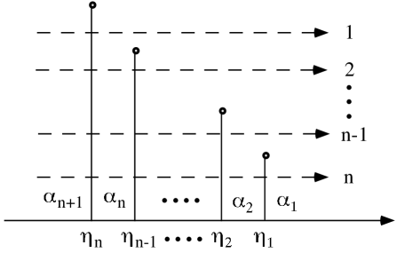
FIG. 2.: The $n$ frequency bands of the spectrum for a background with $n$ transitions frequencies, arranged in decreasing order.

At this point, one remark is in order. The spectral distribution determined through the above procedure applies – by construction – only sufficiently far from the transition frequencies, $k\ll k_{i}$. Near the transition the spectral slope may change with respect to the asymptotic regime, but always in such a way as to guarantee the continuity of the spectrum at $k=k_{i}$. In eq. (31), however, the asymptotic expression has been extrapolated up to $k_{i}$ and, as a consequence, its amplitude is normalized by continuity. This is certainly allowed – within our approximations – when the leading term of the expansion (13) is nonzero. When $\alpha_{i}$ and $\alpha_{1}$ are both smaller than $1/2$, and the leading term is vanishing, this extrapolation may introduce an error in the asymptotic amplitude of the spectrum, which is however of order one – and thus compatible with the degree of accuracy required for our present estimate – provided the amplification of the corresponding band is not too large, i.e. provided $F(k_{i})\equiv(k_{i}/k_{i-1})^{\gamma_{i1}}(k_{i}/k_{1})^{\gamma_{1i}}~{}\raise 1.72218pt\hbox{$<$}\kern-8.00003pt\lower 2.6694pt\hbox{$\sim$}~{}1$. If $F\gg 1$, on the contrary, the correct asymptotic amplitude of the branches with $k<k_{i}$ is obtained by renormalizing the results of eq. (31) by the factor $F^{-2}(k_{i})$.

A recurrent expression, similar to eq. (31), is also obtained for the complementary situation in which the $n$ transition frequencies $k_{i}$ are arranged in decreasing order, for $\eta$ ranging from minus to plus infinity (see Fig. 2). There are still $n$ frequency bands, defined by $k_{i-1}<k<k_{i}$, $i=1,...,n$, and the spectral coefficients can be approximated as follows:

$$|A^{1}_{-}(k)| \simeq x_{n}^{\gamma_{n+1,n}}x_{n}^{\gamma_{n,n+1}},~{}~{}~{}~{}~{}~{}~{}~{}~{}~{}~{}~{}~{}~{}~{}~{}~{}~{}~{}~{}~{}~{}~{}~{}~{}~{}~{}~{}~{}~{}~{}~{}~{}~{}~{}~{}~{}~{}~{}~{}~{}~{}~{}~{}~{}~{}~{}~{}~{}~{}~{}~{}~{}~{}~{}~{}~{}~{}~{}~{}~{}~{}k_{n-1}<k<k_{n}$$ (40)

$$\simeq x_{n}^{\gamma_{n+1,n-1}}x_{n-1}^{\gamma_{n-1,n+1}}\left(\frac{x_{n}}{x_{n-1}}\right)^{\gamma_{n,n+1}}\left(\frac{x_{n}}{x_{n-1}}\right)^{\gamma_{n+1,n}-\gamma_{n+1,n-1}},~{}~{}~{}~{}~{}~{}~{}~{}~{}~{}k_{n-2}<k<k_{n-1}$$ (41)

$$\vdots$$ (42)

$$\simeq x_{n}^{\gamma_{n+1,1}}x_{1}^{\gamma_{1,n+1}}\left(\frac{x_{n}}{x_{n-1}}\right)^{\gamma_{n,n+1}}\left(\frac{x_{n}}{x_{n-1}}\right)^{\gamma_{n+1,n}-\gamma_{n+1,n-1}}$$ (45)

$$\left(\frac{x_{n-1}}{x_{n-2}}\right)^{\gamma_{n-1,n+1}}\left(\frac{x_{n}}{x_{n-2}}\right)^{\gamma_{n+1,n-1}-\gamma_{n+1,n-2}}...\left(\frac{x_{2}}{x_{1}}\right)^{\gamma_{2,n+1}}\left(\frac{x_{n}}{x_{1}}\right)^{\gamma_{n+1,2}-\gamma_{n+1,1}},$$

$$~{}~{}~{}~{}~{}~{}~{}~{}~{}~{}~{}~{}~{}~{}~{}~{}~{}~{}~{}~{}~{}~{}~{}~{}~{}~{}~{}~{}~{}~{}~{}~{}~{}~{}~{}~{}~{}~{}~{}~{}~{}~{}~{}~{}~{}~{}~{}~{}~{}~{}~{}~{}~{}~{}~{}~{}~{}~{}~{}~{}~{}~{}~{}~{}~{}~{}~{}~{}~{}~{}~{}~{}~{}~{}~{}~{}~{}~{}~{}~{}k<k_{1}$$

where $\gamma_{ik}$ are given again by eqs. (33), (LABEL:17). Again, when the leading term is vanishing, the asymptotic amplitudes are correct provided ${\overline{F}}(k_{i})\equiv(k_{i}/k_{i+1})^{\gamma_{i+1,n+1}}(k_{i}/k_{n})^{\gamma_{n+1,i+1}}~{}\raise 1.72218pt\hbox{$<$}\kern-8.00003pt\lower 2.6694pt\hbox{$\sim$}~{}1$, otherwise they are to be renormalized by the factor ${\overline{F}}^{-2}(k_{i})$.

The above results can be summarized by a set of prescriptions, allowing an automatic computation of the spectrum, once the relevant diagram is plotted. For a synthetic formulation of such prescriptions it is convenient to define, for each “leg” of the diagram representing a transition, the so-called phase of exit and phase of re-enter. More precisely, for any leg $\eta_{i}$ placed to the left of the highest one, we shall define phase of re-enter the one directly to the right of the last leg crossed by the transition frequency $k_{i}=|\eta_{\i}|^{-1}$. For any leg $\eta_{j}$ placed to the right of the highest one, we shall define phase of exit the one directly to the left of the first leg crossed by the transition frequency $k_{j}=|\eta_{j}|^{-1}$ (see Fig. 3).

With the above definitions, the diagrammatic rules for the computation of the spectrum can now be synthetized as follows.

• We plot the diagram for the given model of background

• We choose the frequency band we want to compute, and we single out the relevant transitions.

• For any relevant leg $\eta_{i}$ placed to the left of the highest one we insert the amplitude factor:

  $$\left(x_{i-1}\over x_{i}\right)^{\gamma_{ir}}\left(x_{r}\over x_{i}\right)^{\gamma_{ri}-\gamma_{r,i+1}}.$$ (46)

  For any relevant leg $\eta_{i}$ placed to the right of the highest one we insert the factor:

  $$\left(x_{i+1}\over x_{i}\right)^{\gamma_{i+1,e}}\left(x_{e-1}\over x_{i}\right)^{\gamma_{e,i+1}-\gamma_{ei}},$$ (47)

  where the labels $``e"$ and $``r"$ denote, respectively, the exit and re-enter phase (note that, according to these rules, the highest leg does not contribute to the amplitude).

• We add the overal factor determing the frequency dependence of the spectrum:

  $$x_{f}^{\gamma_{f+1,\ell}}x_{\ell}^{\gamma_{\ell,f+1}},$$ (48)

  where the labels $``f"$ and $``\ell"$ denote, respectively, the first and last (from the left) relevant legs for the band we are considering.

• We compute, finally, the powers $\gamma_{ik}$ according to eqs. (33), (LABEL:17) and, if needed, we renormalize the amplitudes through the factors $F^{-2}$ or ${\overline{F}}^{-2}$, as discussed before.

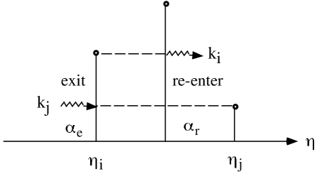
FIG. 3.: A graphic representation of the exit phase for the “leg” $\eta_{j}$, and of the re-enter phase for the “leg” $\eta_{i}$.

As a simple application of such a method, we shall compute here the spectrum for the amplification process represented by the diagram of Fig. 4, by assuming for the various phases the following particular values:

$$\alpha_{1}=1,~{}~{}~{}~{}~{}~{}~{}~{}\alpha_{2}=1/2,~{}~{}~{}~{}~{}~{}~{}~{}\alpha_{3}=2,~{}~{}~{}~{}~{}~{}~{}~{}\alpha_{4}=1/2.$$ (49)

With such a choice of the kinematical powers, the diagram of Fig. 4 may represent (in the Einstein frame) the amplification of tensor metric fluctuations in a non-minimal model of string cosmology [5, 10], which includes an initial dilaton-driven phase ($\eta<\eta_{3}$), a first intermediate, high-curvature string phase ($\eta_{3}<\eta<\eta_{2}$), a second intermediate dilaton phase with decreasing curvature ($\eta_{2}<\eta<\eta_{1}$), and a final radiation-dominated phase, with constant dilaton ($\eta>\eta_{1}$). In the limit $\eta_{2}\rightarrow\eta_{1}$ the model reduces to the minimal one, in the limit $\eta_{3}\rightarrow\eta_{2}$ one recovers instead the non-minimal model discussed in [7].

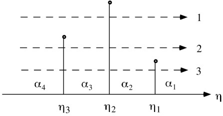
FIG. 4.: An example of diagram representing the amplification of tensor metric perturbations, in a non-minimal model of string cosmology.

Let us consider, for instance, the (lowest frequency) band number $3$ of Fig. 4, corresponding to a “three-leg” transition (for this band, obviously, $\eta_{3}$ is the first leg and $\eta_{1}$ is the last one). For the leg $\eta_{3}$ the re-enter phase is $\alpha_{2}$, for the leg $\eta_{1}$ the exit phase is $\alpha_{4}$. Following the rules listed above we obtain the spectral coefficient

$$|A_{-}^{1}(k)|\simeq x_{3}^{\gamma_{41}}x_{1}^{\gamma_{14}}\left(x_{2}\over x_{3}\right)^{\gamma_{32}}\left(x_{2}\over x_{3}\right)^{\gamma_{23}-\gamma_{24}}\left(x_{2}\over x_{1}\right)^{\gamma_{24}}\left(x_{3}\over x_{1}\right)^{\gamma_{42}-\gamma_{41}},~{}~{}~{}~{}~{}~{}k<k_{3}.$$ (50)

The computation of the powers $\gamma_{ik}$, according to eqs. (33), (LABEL:17), (39), gives:

$$\gamma_{32}\left(2,{1\over 2}\right) =-{3\over 2},~{}~{}~{}~{}~{}~{}~{}~{}~{}\gamma_{23}\left(2,{1\over 2}\right)=0,$$ (51)

$$\gamma_{24}\left({1\over 2},{1\over 2}\right) =0,~{}~{}~{}~{}~{}~{}~{}~{}~{}~{}~{}~{}\gamma_{42}\left({1\over 2},{1\over 2}\right)=0,$$ (52)

$$\gamma_{41}\left({1\over 2},1\right) =0,~{}~{}~{}~{}~{}~{}~{}~{}~{}~{}~{}~{}\gamma_{14}\left({1\over 2},1\right)=-{1\over 2},$$ (53)

where the ordered labels of $\gamma$ refers to the various phases, and the numbers enclosed in round brackets refer to the particular numerical values of the corresponding kinematical powers. The spectral coefficient (50) thus becomes

$$|A_{-}^{1}(k)|\simeq\left(k_{3}\over k_{2}\right)^{-3/2}\left(k\over k_{1}\right)^{-1/2},$$ (54)

and the associated energy distribution (5),

$$\Omega(\omega,t)\simeq{8\over 3\pi}{\omega_{1}^{4}\over M_{p}^{2}H^{2}}\left(\omega_{2}\over\omega_{3}\right)^{3}\left(\omega\over\omega_{1}\right)^{3},$$ (55)

reproduces (modulo logarithmic corrections) the well known cubic slope associated to the dilaton-radiation transiton, and is in agreement with the results of [5] and [10]. With the same procedure we can easily estimate the spectrum for the other bands of Fig. 4.

In summary, we have shown in this paper how to obtain a quick estimate of the cosmological spectra using a simple method, based on a set of effective prescriptions, and on a diagrammatic representation of the amplification of perturbations. We believe that such a method does not represent only a mathematical “curiosity”, but may have useful applications to the study of various inflationary scenarios, that will be discussed in future papers.

REFERENCES

[1]
[2]S. Weinberg, Gravitation and Cosmology (Wiley, New York,
1972).
[3] E. W. Kolb and M. S. Turner, The
Early Universe (Addison-Wesley, Redwood City, CA, 1990);
A. D. Linde, Particle Physics and Inflationary Cosmology (Harwood,
Chur, Switzerland, 1990).
[4]V. F. Mukhanov, H. A. Feldman and R. H.
Brandenberger, Phys. Rep. 215, 203 (1992); A. R. Liddle and D. H.
Lyth, Phys. Rep. 231, 1 (1993).
[5]M. Gasperini, in String theory in curved spacetimes, ed. N.
Sanchez (World Scientific, Singapore, 1998), p. 333.
[6]M. Abramowitz and I. A. Stegun, Handbook of
mathematical functions (Dover, New York, 1972).
[7]A. Buonanno, K. A. Meissner, C. Ungarelli and G. Veneziano, JHEP
001, 004 (1998).
[8]B. Allen, Phys. Rev. D37, 2078 (1988).
[9] R. Brustein, M. Gasperini and G. Veneziano, Phys.
Lett. B431, 277 (1998).