Statistical Mechanics of Relativistic One-Dimensional Self-Gravitating Systems

R.B. Mann and P. Chak

Dept. of Physics, University of Waterloo Waterloo, ONT N2L 3G1, Canada

PACS numbers: 5.20.-y, 04.40.-b 5.90.+m

We consider the statistical mechanics of a general relativistic one-dimensional self-gravitating system. The system consists of $N$-particles coupled to lineal gravity and can be considered as a model of $N$ relativistically interacting sheets of uniform mass. The partition function and one-particle distitrubion functions are computed to leading order in $1/c$ where $c$ is the speed of light; as $c\to\infty$ results for the non-relativistic one-dimensional self-gravitating system are recovered. We find that relativistic effects generally cause both position and momentum distribution functions to become more sharply peaked, and that the temperature of a relativistic gas is smaller than its non-relativistic counterpart at the same fixed energy. We consider the large-$N$ limit of our results and compare this to the non-relativistic case.

1 Introduction

One-dimensional systems of $N$ particles mutually interacting through gravitational forces have been of interest in astrophysics for more than three decades.  While used primarily as prototypes for the behaviour of gravity in higher dimensions, one-dimensional self-gravitating systems (OGS’s) also approximate the behaviour of some physical systems in 3 spatial dimensions. These include the dynamics of stars in a direction orthogonal to the plane of a highly flattened galaxy and the collisions of flat parallel domain walls moving in directions perpendicular to their surfaces. Furthermore, very long-lived core-halo structures in the OGS phase space are known to exist, reminiscent of structures observed in globular clusters, in which a dense massive core in near equilibrium is surrounded by a halo of stars with high kinetic energy that interact only weakly with the core [1].

The statistical properties of the OGS are particularly intriguing.  Despite extensive study, many unanswered questions remain. For example it is not clear if the OGS can attain a true equilibrium state from arbitrary initial conditions.  Its ergodic and equipartition properties are still not well understood.  This is primarily because the particle interactions of the OGS (as with any self-gravitating system) are attractive and cumulatively long range, in strong contrast to typical thermodynamic systems for which such interactions are repulsive and short range. For the OGS the macroscopic  dynamics does not decouple from the microscopic dynamics, and the usual thermodynamic analysis does not apply.

However there are some established features of the OGS. Rybicki [2] derived in closed form the single-particle distribution function in both the canonical and microcanonical ensembles.   In the large $N$ limit these distribution functions reduce to the isothermal solution of the Vlasov equation.

All studies to date have neglected relativistic effects. This limitation is understandable since no relativistic $N$ particle Hamiltonian was available for analysis.  However this situation changed recently when a prescription for obtaining the Hamiltonian for a relativistic one-dimensional self-gravitating system (ROGS) was given by Mann and Ohta [3].  This Hamiltonian can be rigorously derived from a generally covariant system coupling relativistic gravity in one spatial dimension (i.e. a 1+1 dimensional theory of gravity [4]) to $N$ point particles. In the non-relativistic limit, the Hamiltonian reduces to that of the OGS.  Although not available in closed form, the Hamiltonian can be obtained as a series expansion in inverse powers of the speed of light $\ c$ to arbitary order.

We consider in this paper the one-particle distribution function for the ROGS.  Our work here is a natural extension of previous work on the $N$-body problem in relativistic gravity. In three spatial dimensions an exact solution to this problem is known for pure Newtonian gravity (and a series solutions has been constructed for arbitrary $N$). In the general theory of relativity dissipation of energy in the form of gravitational radiation has obstructed progress toward obtaining exact solutions to the $N$-body problem even when $N=2$.  However for the ROGS an exact solution to the $2$-body problem was recently obtained [5], and generalizations including a cosmological constant and/or charge subsequently followed [6, 7, 8]. These solutions include both an explicit expression for the proper separtion of the two bodies as a function of time and an explicit expression for the Hamiltonian for the $2$-body ROGS as a function of the proper separation and the centre-of-inertia momentum of the bodies.

Encouraged by these results, we here begin a first attempt to understand the basic features of the $N$-body ROGS.  We shall recapitulate the canonical formalism used in ref. [3] to derive the Hamiltonian for the $N$-body ROGS.  We then compute the partition function and canonical distribution functions. Using an integral transform we then calculate the microcanonical distribution functions. All results are in closed form to leading order in $1/c$. We consider the limit of large $N$ and compare the ROGS and the OGS. We close with a few remarks. Lengthy intermediate calculations are confined to appendices.

2 Canonical $N$-particle Hamiltonian of the ROGS

The OGS Hamiltonian is

$$H = \sum_{a}\frac{p_{a}^{2}}{2m_{a}}+\pi G\sum_{a}\sum_{b}m_{a}m_{b}\mid z_{a}-z_{b}\mid$$ (1)

$$= \sum_{a}\frac{p_{a}^{2}}{2m_{a}}+2\pi G\sum_{a>b}m_{a}m_{b}\mid z_{a}-z_{b}\mid$$

where the summation is over all $N$ particles, located at positions $z_{a}$ along the spatial axis.  The potential term straightforwardly follows upon solving the Newtonian equation

$$\nabla^{2}\varphi=4\pi G\rho$$ (2)

in one spatial dimension, where $\rho=\sum_{a}m_{a}\delta(x-z_{a})$ is the mass density of the $N$ point particles. Our task in this section is to find a prescription for obtaining a relativistic generalization of (1).

The Hamiltonian for the ROGS that we use is that of a $\left(1+1\right)$ dimensional theory (a lineal gravity theory) that models $\left(3+1\right)$ dimensional general relativity in that it sets the Ricci scalar equal to the trace of the stress-energy of prescribed matter fields and sources. Hence matter governs the evolution of spacetime curvature which reciprocally governs the evolution of matter [4]. We refer to this theory as $R=T$ theory. Apart from being able to model a number of textbook scenarios in general relativity [9], it has the attractive feature of having a consistent Newtonian limit [4]. This limit, essential for our purposes, is problematic in a generic $(1+1)$-dimensional theory of gravity theory [10].

Since the Einstein action is a topological invariant in $(1+1)$ dimensions, a scalar (dilaton) field must be included in the action [11].  Its coupling to the curvature is chosen so that only the trace of the stress energy of matter ($N$ point particles here) is set equal to the Ricci scalar. This action will form the basis for the ROGS we consider. Upon canonical reduction of the action [3], the ROGS Hamiltonian is given in terms of a spatial integral of the second derivative of the dilaton field, which is a function of the coordinates and momenta of the particles and is determined from the constraint equations.

The action integral for the gravitational field coupled to $N$ point particles is

$$I = \int d^{2}x\left[\frac{1}{2\kappa}\sqrt{-g}g^{\mu\nu}\left\{\Psi R_{\mu\nu}+\frac{1}{2}\nabla_{\mu}\Psi\nabla_{\nu}\Psi\right\}\right.$$ (3)

$$\makebox[20.00003pt]{}\left.+\sum_{a}\int d\tau_{a}\left\{-m_{a}\left(-g_{\mu\nu}(x)\frac{dz_{a}^{\mu}}{d\tau_{a}}\frac{dz_{a}^{\nu}}{d\tau_{a}}\right)^{1/2}\right\}\delta^{2}(x-z_{a}(\tau_{a}))\right]\;,$$

where $\Psi$ is the dilaton field, $g_{\mu\nu}$ and $g$ are the metric and its determinant, $R$ is the Ricci scalar, and $\tau_{a}$ is the proper time of $a$-th particle whose mass is $m_{a}$, with $\kappa=8\pi G/c^{4}$. We use $\nabla_{\mu}$ to denote the covariant derivative associated with $g_{\mu\nu}$.

The field equations derived from the action (3) are

$$R-g^{\mu\nu}\nabla_{\mu}\nabla_{\nu}\Psi=0\;,$$ (4)

$$\frac{1}{2}\nabla_{\mu}\Psi\nabla_{\nu}\Psi-\frac{1}{4}g_{\mu\nu}\nabla^{\lambda}\Psi\nabla_{\lambda}\Psi+g_{\mu\nu}\nabla^{\lambda}\nabla_{\lambda}\Psi-\nabla_{\mu}\nabla_{\nu}\Psi=\kappa T_{\mu\nu}+\frac{1}{2}g_{\mu\nu}\Lambda\;,$$ (5)

$$\frac{d}{d\tau_{a}}\left\{g_{\mu\nu}(z_{a})\frac{dz_{a}^{\nu}}{d\tau_{a}}\right\}-\frac{1}{2}g_{\nu\lambda,\mu}(z_{a})\frac{dz_{a}^{\nu}}{d\tau_{a}}\frac{dz_{a}^{\lambda}}{d\tau_{a}}=0\;,$$ (6)

where

$$T_{\mu\nu}=\sum_{a}m_{a}\int d\tau_{a}\frac{1}{\sqrt{-g}}g_{\mu\sigma}g_{\nu\rho}\frac{dz_{a}^{\sigma}}{d\tau_{a}}\frac{dz_{a}^{\rho}}{d\tau_{a}}\delta^{2}(x-z_{a}(\tau_{a}))\;,$$ (7)

is the stress-energy due to the point masses. Eq.(5) guarantees the conservation of $T_{\mu\nu}$. Inserting the trace of Eq.(5) into Eq.(4) yields

$$R-\Lambda=\kappa T_{\;\;\mu}^{\mu}\;.$$ (8)

Eqs. (5), (6) and (8) form a closed sytem of equations for gravity and matter.

In order to obtain the Hamiltonian in canonical form, we first decompose the scalar curvature in terms of the extrinsic curvature $K$ via

$$\sqrt{-g}R=-2\partial_{0}(\sqrt{\gamma}K)+2\partial_{1}[(N_{1}K-\partial_{1}N_{0})/\sqrt{\gamma}]\;,$$ (9)

where the metric is

$$ds^{2}=-N_{0}^{2}dt^{2}+\gamma\left(dx+\frac{N_{1}}{\gamma}dt\right)^{2}\;,$$ (10)

with $K=(2N_{0}\gamma)^{-1}(2\partial_{1}N_{1}-\gamma^{-1}N_{1}\partial_{1}\gamma-\partial_{0}\gamma)$, so that $\gamma=g_{11},N_{0}=(-g^{00})^{-1/2}$ and $N_{1}=g_{10}$. Rewriting the action (3) in first-order form yields

$$I=\int d^{2}x\left\{\sum_{a}p_{a}\dot{z}_{a}\delta(x-z_{a}(t))+\pi\dot{\gamma}+\Pi\dot{\Psi}+N_{0}R^{0}+N_{1}R^{1}\right\}$$ (11)

where $\pi$ and $\Pi$ are the respective conjugate momenta to $\gamma$ and $\Psi$. Here

$$R^{0} = -\kappa\sqrt{\gamma}\gamma\pi^{2}+2\kappa\sqrt{\gamma}\pi\Pi+\frac{1}{4\kappa\sqrt{\gamma}}(\Psi^{\prime})^{2}-\frac{1}{\kappa}\left(\frac{\Psi^{\prime}}{\sqrt{\gamma}}\right)^{\prime}$$

$$-\sum_{a}\sqrt{\frac{p_{a}^{2}}{\gamma}+m_{a}^{2}}\;\delta(x-z_{a}(t))\;,$$

$$R^{1} = \frac{\gamma^{\prime}}{\gamma}\pi-\frac{1}{\gamma}\Pi\Psi^{\prime}+2\pi^{\prime}+\sum_{a}\frac{p_{a}}{\gamma}\delta(x-z_{a}(t))\;,$$ (12)

with the symbols $(\;\dot{}\;)$ and $(\;^{\prime}\;)$ denoting $\partial_{0}$ and $\partial_{1}$, respectively.

Variation of the action (11) yields the set of equations

$$\dot{\pi} + N_{0}\left\{\frac{3\kappa}{2}\sqrt{\gamma}\pi^{2}-\frac{\kappa}{\sqrt{\gamma}}\pi\Pi+\frac{1}{8\kappa\sqrt{\gamma}\gamma}(\Psi^{\prime})^{2}-\sum_{a}\frac{p_{a}^{2}}{2\gamma^{2}\sqrt{\frac{p_{a}^{2}}{\gamma}+m_{a}^{2}}}\;\delta(x-z_{a}(t))\right.$$ (13)

$$+ N_{1}\left\{-\frac{1}{\gamma^{2}}\Pi\Psi^{\prime}+\frac{\pi^{\prime}}{\gamma}+\sum_{a}\frac{p_{a}}{\gamma^{2}}\;\delta(x-z_{a}(t))\right\}+N_{0}^{\prime}\frac{1}{2\kappa\sqrt{\gamma}\gamma}\Psi^{\prime}+N_{1}^{\prime}\frac{\pi}{\gamma}=0\;,$$

$$\dot{\gamma}-N_{0}(2\kappa\sqrt{\gamma}\gamma\pi-2\kappa\sqrt{\gamma}\Pi)+N_{1}\frac{\gamma^{\prime}}{\gamma}-2N_{1}^{\prime}=0\;,$$ (14)

$$R^{0}=0\;,$$ (15)

$$R^{1}=0\;,$$ (16)

$$\dot{\Pi}+\partial_{1}(-\frac{1}{\gamma}N_{1}\Pi+\frac{1}{2\kappa\sqrt{\gamma}}N_{0}\Psi^{\prime}+\frac{1}{\kappa\sqrt{\gamma}}N_{0}^{\prime})=0\;,$$ (17)

$$\dot{\Psi}+N_{0}(2\kappa\sqrt{\gamma}\pi)-N_{1}(\frac{1}{\gamma}\Psi^{\prime})=0\;,$$ (18)

$$\dot{p}_{a}+\frac{\partial N_{0}}{\partial z_{a}}\sqrt{\frac{p_{a}^{2}}{\gamma}+m_{a}^{2}}-\frac{N_{0}}{2\sqrt{\frac{p_{a}^{2}}{\gamma}+m_{a}^{2}}}\frac{p_{a}^{2}}{\gamma^{2}}\frac{\partial\gamma}{\partial z_{a}}-\frac{\partial N_{1}}{\partial z_{a}}\frac{p_{a}}{\gamma}$$

$$\makebox[20.00003pt]{}+N_{1}\frac{p_{a}}{\gamma^{2}}\frac{\partial\gamma}{\partial z_{a}}=0\;,$$ (19)

$$\dot{z_{a}}-N_{0}\frac{\frac{p_{a}}{\gamma}}{\sqrt{\frac{p_{a}^{2}}{\gamma}+m_{a}^{2}}}+\frac{N_{1}}{\gamma}=0\;.$$ (20)

All metric components ($N_{0}$, $N_{1}$, $\gamma$) in equations (19) and (20) are evaluated at the point $x=z_{a}$, where

$$\frac{\partial f}{\partial z_{a}}\equiv\left.\frac{\partial f(x)}{\partial x}\right|_{x=z_{a}}\;.$$

The quantities $N_{0}$ and $N_{1}$ are Lagrange multipliers which yield the constraint equations (15) and (16). The above set of equations can be proved to be equivalent to the set of equations (4), (5) and (6) [3].

An examination of the generator of space and time transformations [3, 5] indicates that we find that we can consistently choose the coordinate conditions

$$\gamma=1\makebox[20.00003pt]{}\mbox{and}\makebox[20.00003pt]{}\Pi=0\;$$ (21)

upon which the action (11) reduces to

$$I=\int d^{2}x\left\{\sum_{a}p_{a}\dot{z}_{a}\delta(x-z_{a})-{\cal H}\right\}\;,$$ (22)

after elimination of the constraints, where

$$H=\int dx{\cal H=-}\frac{1}{\kappa}\int{\cal\triangle}\Psi{\cal\;}$$ (23)

is the Hamiltonian for the ROGS.

The field $\Psi$ is no longer arbitrary, but is instead a function of $z_{a}$ and $p_{a}$ that is determined by solving the constraints which are now

$$\triangle\Psi-\frac{1}{4}(\Psi^{\prime})^{2}+\kappa^{2}\pi^{2}+\kappa\sum_{a=1}^{N}\sqrt{p_{a}^{2}+m_{a}^{2}}\delta(x-z_{a})=0\;,$$ (24)

$$2\pi^{\prime}+\sum_{a=1}^{N}p_{a}\delta(x-z_{a})=0\;.$$ (25)

once the coordinate conditions (21) are imposed.  Equation (24) is an energy-balance equation which states that the energy of the particles plus the (negative) gravitational energy must vanish.  Equation (25) states that the total momentum of the gravitational field and the particles must vanish.  The consistency of this canonical reduction was proved in ref. [3] by showing that the canonical equations of motion derived from the reduced Hamiltonian (23) are identical with the equations (19) and (20) .

Hence the Hamiltonian (23) is a function only of the coordinates and momenta of the $N$ particles in the system.  We turn next to its evaluation.

3 Computation of the ROGS Hamiltonian

Although the constraint equations are straightforward to solve in the regions between the particles, the matching conditions of these solutions at the juncture of the particles are quite non-trivial. For the $2$-body ROGS their enforcement yields an equation which determines the Hamiltonian in terms of the remaining degrees of freedom of the system. While this procedure holds in principle for the $N$-body ROGS, we have not found a tractable means of obtaining an analogous determining equation for the Hamiltonian.

However it is possible to straightforwardly and rigourously construct approximation schemes for computing the ROGS Hamiltonian for $N$ particles. For example, the post-linear approximation is an expansion of the Hamiltonian in powers of the gravitational coupling $\kappa$, obtained by writing

$$\Psi = \kappa\Psi^{(1)}+\kappa^{2}\Psi^{(2)}+\cdot\cdot\cdot$$ (26)

$$\chi = \chi^{(0)}+\kappa\chi^{(1)}+\cdot\cdot\cdot\;\;.$$ (27)

where$\chi$ is defined by $\chi^{\prime}\equiv\pi$. Insertion of these expansions into eqs. (24,25) yields

$$H^{(2)} = \sum_{a}\sqrt{p_{a}^{2}+m_{a}^{2}}+\frac{\kappa}{8}\sum_{a}\sum_{b}\left(\sqrt{p_{a}^{2}+m_{a}^{2}}\sqrt{p_{b}^{2}+m_{b}^{2}}-p_{a}p_{b}\right)\left|r_{ab}\right|$$

$$+\frac{\epsilon\kappa}{8}\sum_{a}\sum_{b}\left(\sqrt{p_{a}^{2}+m_{a}^{2}}\;p_{b}-p_{a}\sqrt{p_{b}^{2}+m_{b}^{2}}\right)r_{ab}$$

$$+\frac{1}{4}\left(\frac{\kappa}{4}\right)^{2}\left\{\sum_{a}\sqrt{p_{a}^{2}+m_{a}^{2}}\left[\sum_{b}p_{b}\left|r_{ab}\right|+\epsilon\;\sum_{b}\sqrt{p_{b}^{2}+m_{b}^{2}}r_{ab}\right]^{2}\right.$$

$$\left.-\sum_{a}p_{a}\left[\sum_{b}p_{b}\left|r_{ab}\right|+\epsilon\;\sum_{b}\sqrt{p_{b}^{2}+m_{b}^{2}}r_{ab}\right]\left[\sum_{c}\sqrt{p_{c}^{2}+m_{c}^{2}}\;\left|r_{ac}\right|+\epsilon\;\sum_{c}p_{c}r_{ac}\right]\right.$$

$$\left.+\sum_{a}\sum_{b}\left[\sqrt{p_{a}^{2}+m_{a}^{2}}\sqrt{p_{b}^{2}+m_{b}^{2}}\;\left|r_{ab}\right|-\epsilon\;p_{a}\sqrt{p_{b}^{2}+m_{b}^{2}}r_{ab}\right]\right.$$

$$\makebox[80.00012pt]{}\left.\times\left[\sum_{c}\sqrt{p_{c}^{2}+m_{c}^{2}}\;\left|r_{bc}\right|+\epsilon\;\sum_{c}p_{c}r_{bc}\right]\right.$$

$$\left.-\sum_{a}\sum_{b}\left[\sqrt{p_{a}^{2}+m_{a}^{2}}\;p_{b}\left|r_{ab}\right|-\epsilon\;p_{a}p_{b}r_{ab}\right]\left[\sum_{c}p_{c}\left|r_{bc}\right|+\epsilon\;\sum_{c}\sqrt{p_{c}^{2}+m_{c}^{2}}r_{bc}\right]\right\}\;\;$$

upon insertion into (23), where $r_{ab}=z_{a}-z_{b}$ is the relative separation between particles $a$ and $b$. It can be shown that the solutions to eqs. (24,25) must satisfy the boundary condition $\Psi^{2}-4\kappa^{2}\chi^{2}=0$ in the regions $\mid x\mid>>\mid z_{a}\mid$ in order for the Hamiltonian to be finite [3].

The $\kappa$-expansion is appropriate for describing relativistic fast-motion of the particles and can be carried out to any desired order. However to compare the ROGS from $R=T$ theory with the OGS, we turn to the post-Newtonian expansion, which is an expansion of the Hamiltonian in powers of $c^{-1}$. Since both $p_{a}^{2}/m_{a}^{2}$ and $\sqrt{\kappa}$ are of the order of $c^{-2}$ all terms up to the order of $c^{-4}$ are included in the post-linear Hamiltonian (LABEL:plinH).  The post-Newtonian Hamiltonian to this order is therefore [3]

$$H = \sum_{a=1}^{N}m_{a}c^{2}+\sum_{a=1}^{N}\frac{p_{a}^{2}}{2m_{a}}+2\pi G\sum_{a>b}^{N}m_{a}m_{b}\left|r_{ab}\right|$$ (29)

$$-\frac{1}{c^{2}}\sum_{a=1}^{N}\frac{p_{a}^{4}}{8m_{a}^{3}}+\frac{\pi G}{c^{2}}\sum_{a=1}^{N}\sum_{b=1}^{N}m_{a}\frac{p_{b}^{2}}{m_{b}}\left|r_{ab}\right|-\frac{2\pi G}{c^{2}}\sum_{a>b}^{N}p_{a}p_{b}\left|r_{ab}\right|$$

$$+\left(\frac{\pi G}{c}\right)^{2}\sum_{a=1}^{N}\sum_{b=1}^{N}\sum_{c=1}^{N}m_{a}m_{b}m_{c}\left[\left|r_{ab}\right|\left|r_{ac}\right|-r_{ab}r_{ac}\right]+\cdots$$

where the explicit powers of $c$ have been restored.

The first term in (29) is the total rest energy of the particles, and the second two terms are the OGS Hamiltonian (1).  The remaining terms are all relativistic corrections to the OGS to order $c^{-2}$.  The first of these corrections is a special-relativistic one, whereas the remaining corrections are due to relativistic gravity in one spatial dimension.  Note that gravity not only modifies the potential to a quadratic form, but also includes couplings between particle momenta and their positions. These features – modifications of the distance behaviour of the potential and position-momentum couplings – are fully analogous to those in general relativity in three spatial dimensions.

We next find the equations of motion for the position of the $a$th particle. This follows straightforwardly from Hamilton’s principle. We have

$$\dot{z}_{a} = \frac{\partial H}{\partial p_{a}}$$ (30)

$$= \frac{p_{a}}{m_{a}}-\frac{1}{c^{2}}\left[\frac{p_{a}^{3}}{2m_{a}^{3}}-\frac{\kappa}{4}\sum_{b=1}^{N}m_{b}\frac{p_{a}}{m_{a}}\left|r_{ab}\right|+\frac{\kappa}{4}\sum_{b=1}^{N}p_{b}\left|r_{ab}\right|\right]$$

and

$$\dot{p}_{a} = -\frac{\partial H}{\partial z_{a}}$$ (31)

$$= -2\pi G\sum_{b=1}^{N}m_{a}m_{b}\varepsilon_{ab}-\frac{1}{c^{2}}\left[\pi G\sum_{b=1}^{N}\left(m_{a}\frac{p_{b}^{2}}{m_{b}}+m_{b}\frac{p_{a}^{2}}{m_{a}}\right)\varepsilon_{ab}-2\pi G\sum_{b=1}^{N}p_{a}p_{b}\varepsilon_{ab}\right.$$

$$\left.+2\left(\pi G\right)^{2}\sum_{b=1}^{N}\sum_{c=1}^{N}m_{a}m_{b}m_{c}\left[\varepsilon_{ab}\left|r_{ac}\right|+\varepsilon_{ab}\left|r_{bc}\right|-r_{ab}\right]\right]$$

where $\varepsilon_{ab}=\left\{\begin{array}[]{cc}1&z_{a}>z_{b}\\ -1&z_{a}<z_{b}\end{array}\right.$ .  We can solve (30) for $p_{a}$:

$$p_{a}=m_{a}\dot{z}_{a}+\frac{1}{c^{2}}\left[m_{a}\frac{\dot{z}_{a}^{3}}{2}+2\pi G\sum_{b=1}^{N}\left(\left(m_{b}m_{a}\dot{z}_{a}-m_{a}m_{b}\dot{z}_{b}\right)\left|r_{ab}\right|\right)\right]+\cdots$$ (32)

and then insert this into the equation (31) for $\dot{p}_{a}:$

$$m_{a}\ddot{z}_{a}+ \frac{1}{c^{2}}\left[m_{a}\ddot{z}_{a}\frac{3\dot{z}_{a}^{2}}{2}-2\pi G\sum_{b=1}^{N}\left(\left(m_{b}m_{a}\ddot{z}_{a}-m_{a}m_{b}\ddot{z}_{b}\right)\left|r_{ab}\right|+\left(m_{b}m_{a}\dot{z}_{a}-m_{a}m_{b}\dot{z}_{b}\right)\varepsilon_{ab}\left(\dot{z}_{a}-\dot{z}_{b}\right)\right)\right]$$ (33)

$$= -2\pi G\sum_{b=1}^{N}m_{a}m_{b}\varepsilon_{ab}-\frac{1}{c^{2}}\left[\pi G\sum_{b=1}^{N}\left(m_{a}m_{b}\left[\dot{z}_{b}^{2}+\dot{z}_{a}^{2}\right]\right)\varepsilon_{ab}-2\pi G\sum_{b=1}^{N}m_{a}m_{b}\dot{z}_{a}\dot{z}_{b}\varepsilon_{ab}\right.$$

$$\left.+2\left(\pi G\right)^{2}\sum_{b=1}^{N}\sum_{c=1}^{N}m_{a}m_{b}m_{c}\left[\varepsilon_{ab}\left|r_{ac}\right|+\varepsilon_{ab}\left|r_{bc}\right|-r_{ab}\right]\right]$$

which simplifies to

$$m_{a}\ddot{z}_{a} = -2\pi G\sum_{b=1}^{N}m_{a}m_{b}\varepsilon_{ab}+\frac{\pi G}{c^{2}}\sum_{b=1}^{N}\left(m_{a}m_{b}\left\{3\dot{z}_{a}^{2}+\left[\dot{z}_{b}-\dot{z}_{a}\right]^{2}\right\}\varepsilon_{ab}\right)$$ (34)

$$-\left(\frac{2\pi G}{c}\right)^{2}\sum_{b=1}^{N}\sum_{c=1}^{N}m_{a}m_{b}m_{c}\left(\varepsilon_{ac}-\varepsilon_{bc}\right)\left|r_{ab}\right|$$

$$-2\left(\frac{\pi G}{c}\right)^{2}\sum_{b=1}^{N}\sum_{c=1}^{N}m_{a}m_{b}m_{c}\left[\varepsilon_{ab}\left|r_{ac}\right|+\varepsilon_{ab}\left|r_{bc}\right|-r_{ab}\right]$$

upon an iterative substitution of $\ddot{z}_{a}$ in powers of $c^{-1}$. These equations of motion reduce to those of the OGS in the limit $c\rightarrow\infty$ , and may be shown to be equivalent to the geodesic equations to this order [3].

We wish to investigate the instrinsic structure of the system described by the Hamiltonian (29) .  However because of the translation invariance of the system, two phase-space degrees of freedom are redundant, and so must be factored out; otherwise certain average properties such as density would be uniform throughout space.

Using equation(31), it is straightforward to show that

$$\sum_{a=1}^{N}\dot{p}_{a}=0$$ (35)

and (using also (30) ) that the Hamiltonian is time-independent.  This means that we can perform the phase-space integration subject to the constraint

$$\bar{p}=0\mbox{\ \ \ \ \ \ \ \ \ \ \ where \ \ \ \ \ \ }\overline{p}\equiv\sum_{a=1}^{N}p_{a}$$ (36)

since we can choose a frame of reference in which the centre of inertia is constant.

Removing the redundant position degree-of-freedom is somewhat more delicate. Although the system is invariant under the translation $z_{a}\rightarrow z_{a}+\hat{z}$, eq. (32) implies

$$\overline{p}\equiv\frac{1}{N}\mbox{\ }\sum_{a=1}^{N}p_{a}=\frac{1}{N}\mbox{\ }\sum_{a=1}^{N}\left[m_{a}\dot{z}_{a}\left(1+\frac{1}{2}\frac{\dot{z}_{a}^{2}}{c^{2}}\right)\right]$$ (37)

which cannot be written as a total time derivative.  Physically, the centre of inertia is the relativistically well-defined concept, whereas the centre of mass is not.  However we can deal with this problem by inserting a factor of unity in all phase-space averages in the form

$$\int_{-\infty}^{\infty}dL\,\delta\left(\overline{z}-L\right)$$

where $\overline{z}\equiv\frac{1}{M}\sum_{a=1}^{N}m_{a}z_{a}$ , with $M=$ $\sum_{a=1}^{N}m_{a}$.  If the $L$-dependence of any integral trivially factors out (or can be removed by a shift of variable in the integrand), then we regard the remaining quantity as the physically relevant one to describe the system.

For a canonical ensemble, all phase-space averages are carried out with a weighting function $\exp\left[-\beta H\right]$, where $k_{B}T=\beta^{-1}$ is the temperature multiplied by Boltzmann’s constant $k_{B}$.  For the microcanonical ensemble, an additional constraint of fixed total energy

$$H(z_{a},p_{a})=E$$

must be included, consistent with the time-independence of the Hamiltonian (29) .  Since the system is in momentum isolation, it  is difficult to see how it can be in energy contact with a heat bath, and so the physical relevance of the canonical ensemble is somewhat unclear.  However an evaluation of quantities within the canonical ensemble is instructive in its own right and is a necessary preliminary to computing quantities in the more realistic microcanonical ensemble, and so we include it in the present discussion.

Henceforth we set $m_{a}=m$, so that $M=Nm$.

4 The Canonical Ensemble

We consider in this section the relativistic corrections to the canonical one-particle distribution function $f_{c}^{R}(p,z)$, which is defined to be the phase-space average of the quantity

$$\frac{1}{N}\sum_{a}\delta\left(z-z_{a}\right)\delta\left(p-p_{a}\right)$$ (38)

weighted by $\exp\left(-\beta H\right)$ with the constraint $\hat{p}=0.$ Hence

$$f_{c}^{R}(p,z)=\frac{1}{{\cal Z}N!}\int\int d{\bf p}d{\bf z}\delta\left(\overline{p}\right)\int_{-\infty}^{\infty}dL\,\delta\left(\overline{z}-L\right)\exp\left(-\beta H\right)N^{-1}\sum_{a}\delta\left(z-z_{a}\right)\delta\left(p-p_{a}\right)$$ (39)

where

$${\cal Z}=\frac{1}{N!}\int\int d{\bf p}d{\bf z}\delta\left(\overline{p}\right)\int_{-\infty}^{\infty}dL\,\delta\left(\overline{z}-L\right)\exp\left(-\beta H\right)$$ (40)

is the partition function and where the 2nd line in (39) follows from the indistinguishability of the particles.  Note that a shift of integration variable

$$z_{a}^{\prime}=z_{a}+L$$

renders the partition function in the form

$${\cal Z}=\frac{1}{N!}\int_{-\infty}^{\infty}dL\,\int\int d{\bf p}d{\bf z}^{\prime}\delta\left(\overline{p}\right)\delta\left(\overline{z}^{\prime}\right)\exp\left(-\beta H\right)$$ (41)

where the $L$-dependence is seen to trivially factor out. It can therefore be dropped (along with the prime notation) from further consideration in the evaluation of ${\cal Z}$. Similarly, the single-particle distribution function becomes

$$f_{c}^{R}(p,z)=\frac{1}{{\cal Z}N!}\int_{-\infty}^{\infty}dL\,\int\int d{\bf p}d{\bf z}\delta\left(\overline{p}\right)\delta\left(\overline{z}^{\prime}\right)\exp\left(-\beta H\right)N^{-1}\sum_{a}\delta\left(z-L-z_{a}^{\prime}\right)\delta\left(p-p_{a}\right)$$ (42)

which is of the form $\int_{-\infty}^{\infty}dL\,f_{c}^{\prime R}(p,z-L)$.  We therefore regard $\,f_{c}^{\prime R}(p,z-L)$ as the physically relevant quantity, where

$$f_{c}^{\prime R}(p,z)=\frac{1}{{\cal Z}N!}\int\int d{\bf p}d{\bf z}\delta\left(\overline{p}\right)\delta\left(\overline{z}^{\prime}\right)\exp\left(-\beta H\right)N^{-1}\sum_{a}\delta\left(z-z_{a}^{\prime}\right)\delta\left(p-p_{a}\right)$$ (43)

and where the primes will hencefore be dropped.

Unlike the non-relativistic case, neither the partition function nor $f_{c}^{R}(p,z)$ are separable. We proceed by first evaluating the partition function.

We first write the Hamiltonian (29) in the following form

$$H = Mc^{2}+H_{0}+\frac{1}{c^{2}}H_{R}$$ (44)

$$H_{0} = \sum_{a=1}^{N}\frac{p_{a}^{2}}{2m}+2\pi Gm^{2}\sum_{a>b}^{N}\left|r_{ab}\right|$$ (45)

$$H_{R} = -\sum_{a=1}^{N}\frac{p_{a}^{4}}{8m^{3}}+\pi G\sum_{a=1}^{N}\sum_{b=1}^{N}p_{b}^{2}\left|r_{ab}\right|-2\pi G\sum_{a>b}^{N}p_{a}p_{b}\left|r_{ab}\right|$$ (46)

$$+\left(\pi G\right)^{2}\sum_{a=1}^{N}\sum_{b=1}^{N}\sum_{c=1}^{N}m^{3}\left[\left|r_{ab}\right|\left|r_{ac}\right|-r_{ab}r_{ac}\right]$$

so that

$$\exp\left(-\beta H\right)=e^{-\beta Mc^{2}}e^{-\beta H_{0}}\left(1-\frac{\beta}{c^{2}}H_{R}\right)+{\cal O}\left(\frac{\beta^{2}}{c^{4}}\right)$$ (47)

which is valid to the order in which we are working.  Writing

$$\delta\left(\overline{p}\right)=\frac{1}{2\pi}\int dk\exp\left[ik\sum_{a=1}^{N}p_{a}\right]$$ (48)

we have

$${\cal Z=}\frac{e^{-\beta Mc^{2}}}{N!}\,\int d{\bf z}\delta\left(\overline{z}\right)\exp\left(-2\pi G\beta m^{2}\sum_{a>b}^{N}\left|r_{ab}\right|\right)\int\frac{dk}{2\pi}\int d{\bf p}\exp\left(ik\sum_{a=1}^{N}p_{a}-\beta\sum_{a=1}^{N}\frac{p_{a}^{2}}{2m}\right)\left(1-\frac{\beta}{c^{2}}H_{R}\right)$$ (49)

4.1
The Partition Function

Consider first the integral

$$\int\frac{dk}{2\pi}\int d{\bf p}\exp\left(ik\sum_{a=1}^{N}p_{a}-\beta\sum_{a=1}^{N}\frac{p_{a}^{2}}{2m}\right)\left(1-\frac{\beta}{c^{2}}H_{R}\right)$$ (50)

which has integrals that are at most quartic in the momenta. Straightforward Gaussian integration yields

$$\int\frac{dk}{2\pi}\int d{\bf p}\exp\left(ik\sum_{c=1}^{N}p_{c}-\beta\sum_{c=1}^{N}\frac{p_{c}^{2}}{2m}\right)\left\{\begin{array}[]{c}1\\ p_{a}p_{b}\\ p_{a}^{4}\end{array}\right\}=\frac{1}{\sqrt{N}}\left(\frac{2\pi m}{\beta}\right)^{\left(N-1\right)/2}\left\{\begin{array}[]{c}1\\ \left(\frac{m}{\beta}\right)\times\left\{\begin{array}[]{c}\frac{N-1}{N}\mbox{ \ \ \ }a=b\\ -\frac{1}{N}\mbox{ \ \ \ }a\neq b\end{array}\right.\\ \left(\frac{m}{\beta}\right)^{2}\frac{3\left(N-1\right)^{2}}{N^{2}}\end{array}\right\}$$ (51)

Hence we obtain

$$\int\frac{dk}{2\pi}\int d{\bf p}\exp\left(ik\sum_{a=1}^{N}p_{a}-\beta\sum_{a=1}^{N}\frac{p_{a}^{2}}{2m}\right)\left(1-\frac{\beta}{c^{2}}H_{R}\right)$$

$$= \frac{1}{\sqrt{N}}\left(\frac{2\pi m}{\beta}\right)^{\left(N-1\right)/2}\left\{\left(1-\frac{\beta}{c^{2}}\left(\pi G\right)^{2}\sum_{a=1}^{N}\sum_{b=1}^{N}\sum_{c=1}^{N}m^{3}\left[\left|r_{ab}\right|\left|r_{ac}\right|-r_{ab}r_{ac}\right]\right)\right.$$

$$\left.-\frac{\pi G\beta}{c^{2}}\left(\frac{m}{\beta}\right)\frac{N-1}{N}\sum_{a=1}^{N}\sum_{b=1}^{N}\left|r_{ab}\right|+\frac{2\pi G\beta}{c^{2}}\left(-\frac{m}{N\beta}\right)\sum_{a>b}^{N}\left|r_{ab}\right|+\frac{\beta}{8m^{3}c^{2}}\frac{3\left(N-1\right)^{2}}{N^{2}}\left(\frac{m}{\beta}\right)^{2}\left(\sum_{a=1}^{N}1\right)\right\}$$

$$= \left(1-\frac{\beta\left(\pi G\right)^{2}}{c^{2}}\sum_{a=1}^{N}\sum_{b=1}^{N}\sum_{c=1}^{N}m^{3}\left[\left|r_{ab}\right|\left|r_{ac}\right|-r_{ab}r_{ac}\right]-\frac{2\pi Gm}{c^{2}}\sum_{a>b}^{N}\left|r_{ab}\right|+\frac{3\left(N-1\right)^{2}}{8N\beta mc^{2}}\right)\frac{1}{\sqrt{N}}\left(\frac{2\pi m}{\beta}\right)^{\left(N-1\right)/2}$$

We next consider the integration over the spatial variables. Introducing

$$u_{l}=z_{l+1}-z_{l}\mbox{ \ }1\leq l\leq N\mbox{ \ \ \ \ \ \ \ \ \ }u_{N}=\frac{1}{N}\sum_{m=1}^{N}z_{m}$$ (53)

we have

$$\sum_{a>b}^{N}\left|r_{ab}\right|=\frac{1}{2}\sum_{a=1}^{N}\sum_{b=1}^{N}\left|r_{ab}\right|=\sum_{l=1}^{N-1}l\left(N-l\right)\left(z_{l+1}-z_{l}\right)=\sum_{l=1}^{N-1}l\left(N-l\right)u_{l}$$ (54)

where without loss of generality the particles are ordered in the sequence $z_{1}\leq z_{2}\leq\cdots\leq z_{N}$, and the overall result is then multiplied by ${\bf N!}$  This gives

$$\int d{\bf z\delta\left(\overline{z}\right)\,{\sf F}(z)} = {\bf N!}\int_{-\infty}^{\infty}dz_{1}\int_{z_{1}}^{\infty}dz_{2}\int_{z_{2}}^{\infty}dz_{3}\cdots\int_{z_{N-1}}^{\infty}dz_{N}\,\delta\left(\overline{z}\right){\bf{\sf F}(z)}$$ (55)

$$= {\bf N!}\int_{-\infty}^{\infty}du_{N}\int_{0}^{\infty}du_{1}\int_{0}^{\infty}du_{2}\cdots\int_{0}^{\infty}du_{N-1}\delta\left(u_{N}\right)\,{\bf{\sf F}(u)}$$

$$= {\bf N!}\int d{\bf u\,{\sf F}(u)}$$

provided the function ${\bf{\sf F}(z)}$ is symmetric under interchange of any pair of variables, which is the case here.  The inverse transformation reads

$$z_{n}=u_{N}-\frac{1}{N}\sum_{l=n}^{N-1}D_{n,l}\mbox{ \ \ \ where }D_{n,l}=\left\{\begin{array}[]{l}-l\mbox{ \ \ \ \ \ \ \ \ }n>l\\ N-l\mbox{ \ \ \ }n\leq l\end{array}\right.\mbox{ }$$ (56)

and so we have

$$\sum_{a=1}^{N}\sum_{b=1}^{N}\sum_{c=1}^{N}\left[\left|r_{ab}\right|\left|r_{ac}\right|-r_{ab}r_{ac}\right] = 2\left(\sum_{b>a>c}^{N}r_{ba}r_{ac}+\sum_{b>a>c}^{N}r_{ca}r_{ab}\right)$$ (57)

$$= 4\sum_{k=1}^{N-2}\sum_{l=k+1}^{N-1}\left(N-l\right)\left(l-k\right)ku_{l}u_{k}$$

Consequently the partition function is

$${\cal Z} = \frac{e^{-\beta Mc^{2}}}{\sqrt{N}}\left(\frac{2\pi m}{\beta}\right)^{\left(N-1\right)/2}\int_{0}^{\infty}du_{1}\int_{0}^{\infty}du_{2}\cdots\int_{0}^{\infty}du_{N-1}\exp\left(-2\pi G\beta m^{2}\sum_{n=1}^{N-1}n\left(N-n\right)u_{n}\right)$$

$$\mbox{ }\times\left(1-\frac{4\beta m^{3}}{c^{2}}\left(\pi G\right)^{2}\sum_{k=1}^{N-2}\sum_{l=k+1}^{N-1}\left(N-l\right)\left(l-k\right)ku_{l}u_{k}-\frac{2\pi Gm}{c^{2}}\sum_{l=1}^{N-1}l\left(N-l\right)u_{l}+\frac{3\left(N-1\right)^{2}}{8N\beta mc^{2}}\right)$$

The three basic integrals in (LABEL:can19) are

$$\int d{\bf u}\exp\left(-\lambda\sum_{n=1}^{N-1}n\left(N-n\right)u_{n}\right) = \frac{1}{\lambda^{N-1}\left[\left(N-1\right)!\right]^{2}}$$ (59)

$$\int d{\bf u}\sum_{l=1}^{N-1}k\left(N-k\right)u_{k}\exp\left(-\lambda\sum_{n=1}^{N-1}n\left(N-n\right)u_{n}\right) = \frac{N-1}{\lambda^{N}\left[\left(N-1\right)!\right]^{2}}$$ (60)

$$\int d{\bf u}\sum_{k=1}^{N-2}\sum_{l=k+1}^{N-1}\left(N-l\right)\left(l-k\right)ku_{l}u_{k}\exp\left(-\lambda\sum_{n=1}^{N-1}n\left(N-n\right)u_{n}\right) = \frac{\sum_{k=1}^{N-2}\sum_{l=k+1}^{N-1}\frac{\left(l-k\right)}{l\left(N-k\right)}}{\lambda^{N+1}\left[\left(N-1\right)!\right]^{2}}\mbox{ \ \ \ \ \ \ \ }$$ (61)

yielding

$${\cal Z} = e^{-\beta Mc^{2}}\frac{1}{\sqrt{N}}\left(\frac{2\pi m}{\beta}\right)^{\left(N-1\right)/2}\left(\frac{1+\frac{3\left(N-1\right)^{2}}{8N\beta mc^{2}}}{\left(2\pi G\beta m^{2}\right)^{N-1}\left[\left(N-1\right)!\right]^{2}}\right.$$ (62)

$$\mbox{ \ \ \ }\left.-\frac{4\beta}{c^{2}}\frac{\left(\pi G\right)^{2}m^{3}}{\left(2\pi G\beta m^{2}\right)^{N+1}\left[\left(N-1\right)!\right]^{2}}\sum_{k=1}^{N-1}\sum_{l=k+1}^{N-1}\frac{\left(l-k\right)}{l\left(N-k\right)}-\frac{2\pi Gm}{c^{2}}\frac{N-1}{\left(2\pi G\beta m^{2}\right)^{N}\left[\left(N-1\right)!\right]^{2}}\right)$$

$$= \frac{e^{-\beta Mc^{2}}\left(\frac{2\pi m}{\beta}\right)^{\left(N-1\right)/2}}{\sqrt{N}\left(2\pi G\beta m^{2}\right)^{N-1}\left[\left(N-1\right)!\right]^{2}}\left[1-\frac{1}{\beta mc^{2}}\left\{\frac{\left(5N+3\right)\left(N-1\right)+8N\sum_{k=1}^{N-1}\sum_{l=k+1}^{N-1}\frac{\left(l-k\right)}{l\left(N-k\right)}}{8N}\right\}\right]$$

$$= \frac{\exp\left[-\beta Mc^{2}-\frac{3\left(N-1\right)}{2}\ln\left(\beta mc^{2}\right)-\left\{\frac{\left(5N+3\right)\left(N-1\right)+8N\sum_{k=1}^{N-1}\sum_{l=k+1}^{N-1}\frac{\left(l-k\right)}{l\left(N-k\right)}}{8N\beta mc^{2}}\right\}\right]}{\sqrt{N}\left(\sqrt{2\pi}G/c^{3}\right)^{\left(N-1\right)}\left[\left(N-1\right)!\right]^{2}}\mbox{ }$$

which is the partition function to lowest relativistic order.  The average energy is

$$\left\langle E\right\rangle = -\frac{\partial}{\partial\beta}\ln{\cal Z}$$ (63)

$$= Mc^{2}+\frac{3}{2}\left(N-1\right)\beta^{-1}-\left\{\frac{\left(5N+3\right)\left(N-1\right)+8N\sum_{k=1}^{N-1}\sum_{l=k+1}^{N-1}\frac{\left(l-k\right)}{l\left(N-k\right)}}{8Mc^{2}}\right\}\beta^{-2}\mbox{ \ \ \ \ \ \ \ \ \ \ \ \ \ \ \ }$$

to the relevant order in $c^{-2}$. The relativistic correction grows quadratically with $N$ (for fixed $M=Nm$) and is negative.  Hence the average energy of  a relativistic gravitating system is lower than its non-relativistic counterpart at the same temperature.

4.2
The Single-particle Distribution Function

Consider next the one-particle distribution function, which is

$$f_{c}^{R}(p,z)=\frac{1}{N}\sum_{n=1}^{N}f_{cn}^{R}(p,z)$$ (64)

where

$$f_{cn}^{R}(p,z) = \frac{e^{-\beta Mc^{2}}}{{\cal Z}N!}\int d{\bf z}\delta\left(\overline{z}\right)\exp\left(-2\pi G\beta m^{2}\sum_{a>b}^{N}\left|r_{ab}\right|\right)\delta\left(z-z_{n}\right)$$

$$\mbox{ \ \ \ \ \ }\times\int\frac{dk}{2\pi}\int d{\bf p}\exp\left(ik\sum_{a=1}^{N}p_{a}-\beta\sum_{a=1}^{N}\frac{p_{a}^{2}}{2m}\right)\left(1-\frac{\beta}{c^{2}}H_{R}\right)\delta\left(p-p_{n}\right)$$

$$= \frac{e^{-\beta Mc^{2}}}{{\cal Z}}\int_{-\infty}^{\infty}du_{N}\int_{0}^{\infty}du_{1}\int_{0}^{\infty}du_{2}\cdots\int_{0}^{\infty}du_{N-1}\delta\left(u_{N}\right)\exp\left(-2\pi G\beta m^{2}\sum_{l=1}^{N-1}l\left(N-l\right)u_{l}\right)$$

$$\mbox{ \ \ \ \ \ \ \ \ \ \ \ \ \ \ }\times\delta\left(z-u_{N}+\frac{1}{N}\sum_{l=1}^{N-1}D_{n,l}u_{l}\right)\theta_{cn}(p,{\bf z})$$

$$= \frac{e^{-\beta Mc^{2}}}{{\cal Z}}\int_{0}^{\infty}du_{1}\cdots\int_{0}^{\infty}du_{N-1}\exp\left(-2\pi G\beta m^{2}\sum_{l=1}^{N-1}C_{l}u_{l}\right)\delta\left(z+\frac{1}{N}\sum_{l=1}^{N-1}D_{n,l}u_{l}\right)\theta_{cn}(p,{\bf z})$$

in which

$$\theta_{cn}(p,{\bf z})=\int\frac{dk}{2\pi}\int d{\bf p}\exp\left(ik\sum_{a=1}^{N}p_{a}-\beta\sum_{a=1}^{N}\frac{p_{a}^{2}}{2m}\right)\left(1-\frac{\beta}{c^{2}}H_{R}\right)\delta\left(p-p_{n}\right)$$ (66)

and

$$C_{l}=l\left(N-l\right)\mbox{ \ \ \ \ \ \ \ \ \ \ \ \ \ \ \ }D_{n,l}=\left\{\begin{array}[]{l}\left(N-l\right)\mbox{ \ \ \ \ \ }n\leq l\\ -l\mbox{\ \ \ \ \ \ \ \ \ \ \ \ \ \ \ \ }n>l\end{array}\right.$$ (67)

where eq. (53) has been used to express

$$z_{n}=u_{N}+\frac{1}{N}\sum_{l=1}^{N-1}lu_{l}-\sum_{l=n}^{N-1}u_{l}=u_{N}-\frac{1}{N}\sum_{l=1}^{N-1}D_{n,l}u_{l}$$ (68)

Evaluation of $\theta_{cn}(p,{\bf z})$ is somewhat lengthy, and so we relegate its computation to the appendix.  We obtain

$$\theta_{cn}(p,{\bf z}) = \frac{1}{\sqrt{N-1}}\exp\left(-\frac{N\beta p^{2}}{2m\left(N-1\right)}\right)\left(\frac{2\pi m}{\beta}\right)^{\left(N-2\right)/2}$$

$$\times\left\{\left(1-\frac{\beta m\left(\pi Gm\right)^{2}}{c^{2}}\sum_{a=1}^{N}\sum_{b=1}^{N}\sum_{c=1}^{N}\left[\left|r_{ab}\right|\left|r_{ac}\right|-r_{ab}r_{ac}\right]\right)\right.$$

$$+\frac{1}{2\beta mc^{2}}\left[\frac{\beta^{2}p^{4}N\left(N^{2}-3N+3\right)}{(2m)^{2}\left(N-1\right)^{3}}+\frac{3\beta p^{2}\left(N-2\right)}{2m\left(N-1\right)^{5/2}}+\frac{3\left(N-2\right)^{2}}{4\left(N-1\right)^{3/2}}\right]$$

$$+\left(\frac{\mbox{2}\pi mG}{c^{2}}\right)\left[-\frac{1}{2}\sum_{a=1}^{N}\sum_{b=1}^{N}\left|r_{ab}\right|-\left(\frac{N^{2}\beta p^{2}}{2m\left(N-1\right)^{2}}-\frac{N}{2(N-1)}\right)\left(\sum_{c=1}^{N}\left|r_{cn}\right|\right)\right]$$

or alternatively, in terms of the ${\bf u}$ variables

$$\theta_{cn}(p,{\bf u}) = \frac{1}{\sqrt{N-1}}\exp\left(-\frac{N\beta p^{2}}{2m\left(N-1\right)}\right)\left(\frac{2\pi m}{\beta}\right)^{\left(N-2\right)/2}$$

$$\times\left\{\left(1-\frac{4\beta m\left(\pi Gm\right)^{2}}{c^{2}}\sum_{k=1}^{N-2}\sum_{l=k+1}^{N-1}\left(N-l\right)\left(l-k\right)ku_{l}u_{k}\right)\right.$$

$$+\frac{1}{2\beta mc^{2}}\left[\frac{\beta^{2}p^{4}N\left(N^{2}-3N+3\right)}{(2m)^{2}\left(N-1\right)^{3}}+\frac{3\beta p^{2}\left(N-2\right)}{2m\left(N-1\right)^{5/2}}+\frac{3\left(N-2\right)^{2}}{4\left(N-1\right)^{3/2}}\right]$$

$$-\left(\frac{2\pi mG}{c^{2}}\right)\left[\sum_{l=1}^{N-1}l\left(N-l\right)u_{l}+\left(\frac{N^{2}\beta p^{2}}{2m\left(N-1\right)^{2}}-\frac{N}{2(N-1)}\right)\left(\sum_{s=1}^{n-1}su_{s}+\sum_{s=n}^{N-1}(N-s)u_{s}\right)\right]$$

Now consider eq. (4.2), which can be rewritten as

$$f_{cn}^{R}(p,z)=\frac{e^{-\beta Mc^{2}}}{{\cal Z}}\int\frac{dk}{2\pi}\int d{\bf u}\exp\left(-ikz-\lambda\beta\sum_{l=1}^{N-1}\left(C_{l}+i\alpha D_{nl}\right)u_{l}\right)\theta_{cn}(p,{\bf u})$$ (71)

where

$$\lambda=2\pi Gm^{2}\mbox{ \ \ \ \ }\alpha=\frac{k}{N\beta\lambda}\mbox{ }$$ (72)

The integration now involves straightforward integrations over the ${\bf u}$ variables, after which an evaluation of the $k$-integral using Jordan’s lemma must be performed.  This involves some rather tedious manipulations which we describe in appendix ???  The final result is

$$f_{cn}(p,z) = \frac{\left(2\pi Gm^{2}\right)\left(N\beta\right)^{3/2}}{\sqrt{2\pi m\left(N-1\right)}}\exp\left[\frac{1}{\beta mc^{2}}\left\{\frac{(5N+3)\left(N-1\right)}{8N}+\sum_{k=1}^{N-1}\sum_{l=k+1}^{N-1}\frac{\left(l-k\right)}{l\left(N-k\right)}\right\}\right]$$

$$\mbox{ \ }\times\sum_{l=1}^{N-1}\left[\left\{A_{l}^{N}\left(1+\frac{1}{2\beta mc^{2}}\left(\frac{\beta^{2}p^{4}\left(1+\left(N-1\right)^{3}\right)}{\left(2m\right)^{2}\left(N-1\right)^{3}}+\frac{3\left(N-2\right)\beta p^{2}}{2m\left(N-1\right)^{2}}+\frac{3\left(N-2\right)^{2}}{4\left(N-1\right)}\right)\right)\right.\right.$$

$$\mbox{\ }-\frac{1}{\beta mc^{2}}\left[B_{l}^{N}-A_{l}^{N}\left(1-2N\left(\beta\pi Gm^{2}\right)l\left|z\right|\right)\right]$$

$$+\frac{2}{\beta mc^{2}}\left(\frac{N}{2\left(N-1\right)}-\frac{\beta p^{2}}{2m}\left[\frac{N^{2}}{\left(N-1\right)^{2}}\right]\right)\mbox{\ }\left[C_{l}^{N}-\frac{1}{l}A_{l}^{N}\left(1-2N\left(\beta\pi Gm^{2}\right)l\left|z\right|\right)\right]$$

$$\mbox{ \ \ \ \ }\left.\left.-\frac{1}{\beta mc^{2}}\left[D_{l}^{N}+K_{l}^{N}\left(1-2N\left(\beta\pi Gm^{2}\right)l\left|z\right|\right)\right]\right\}\exp\left(-\frac{N\beta p^{2}}{2m\left(N-1\right)}-2\pi GN\beta m^{2}l\left|z\right|\right)\right]\mbox{ \ \ }$$

Integration over $p$ yields the canonical density distribution function

$$\rho_{c}\left(z\right) = \int_{-\infty}^{\infty}dpf_{cn}(p,z)$$ (74)

$$= \left(2\pi Gm^{2}N\beta\right)\exp\left[\frac{1}{\beta mc^{2}}\left\{\frac{(5N+3)\left(N-1\right)}{8N}+\sum_{k=1}^{N-1}\sum_{l=k+1}^{N-1}\frac{\left(l-k\right)}{l\left(N-k\right)}\right\}\right]$$

$$\times\sum_{l=1}^{N-1}\left\{A_{l}^{N}+\frac{1}{\beta mc^{2}}\left(\frac{3}{8}\frac{\left(N-1\right)^{2}}{N}A_{l}^{N}-B_{l}^{N}-D_{l}^{N}\right)\right.$$

$$\mbox{ \ \ \ \ \ \ \ \ \ \ \ \ \ }\left.+\frac{1}{\beta mc^{2}}\left[A_{l}^{N}-K_{l}^{N}\right]\left(1-2\pi Gm^{2}N\beta l\left|z\right|\right)\right\}\exp\left(-2\pi Gm^{2}N\beta l\left|z\right|\right)\mbox{ \ \ \ \ \ }$$

whereas integration over $z$ yields the canonical momentum distribution function

$$\vartheta_{cn}(p) = \int_{-\infty}^{\infty}dz\,f_{cn}(p,z)$$ (75)

$$= \sqrt{\frac{\left(N\beta\right)}{2\pi m\left(N-1\right)}}\exp\left[-\frac{N\beta p^{2}}{2m\left(N-1\right)}\right]$$

$$\times\left(1+\frac{1}{\beta mc^{2}}\left(\frac{N\beta^{2}p^{4}\left(N^{2}-3N+3\right)}{8m^{2}\left(N-1\right)^{3}}-\frac{\beta p^{2}\left(4N^{2}-7N+6\right)}{4m\left(N-1\right)^{2}}+\frac{5N(N-1)+3}{8N\left(N-1\right)}\right)\right)\mbox{ \ \ \ \ }$$

From the results in the appendix, it can be shown that

$$\sum_{l=1}^{N-1}\frac{1}{l}A_{l}^{N}=\frac{1}{2}\mbox{ \ \ \ \ \ }\sum_{l=1}^{N-1}\frac{1}{l}B_{l}^{N}=\frac{1}{2}\mbox{ }\left(N-1\right)\mbox{ \ \ \ \ \ }\sum_{l=1}^{N-1}\frac{1}{l}C_{l}^{N}=\frac{\left(N-1\right)}{N}\mbox{\ \ \ \ \ \ }\sum_{l=1}^{N-1}\frac{1}{l}D_{l}^{N}=\frac{1}{2}\sum_{k=1}^{N-1}\sum_{l=k+1}^{N-1}\frac{\left(l-k\right)}{l\left(N-k\right)}$$ (76)

which can be used to show that

$$\int_{-\infty}^{\infty}dz\,\rho_{c}\left(z\right)=1\mbox{ \ \ \ and \ \ \ }\int_{-\infty}^{\infty}dp\vartheta_{cn}(p)=1$$ (77)

We also have the relations

$$\sum_{l=1}^{N-1}A_{l}^{N}=\frac{1}{2}\frac{N-1}{2N-3}\mbox{ \ \ \ \ \ \ \ \ \ \ \ }\sum_{l=1}^{N-1}B_{l}^{N}=\frac{1}{2}\frac{\left(N-1\right)^{2}}{2N-3}$$ (78)

the first of which was demonstrated by Rybicki [2].

5
The Microcanonical Ensemble

The results for the canonical ensemble obtained in the previous section are for a system of relativistic gravitating particles coupled to a heat bath which keeps the system at a constant temperature $T=\beta^{-1}$.   In such a situation the energy of the system ill-defined, and undergoes fluctuations of the order $kT$.  An isolated system, on the other hand, would have its total energy conserved, and this is the more realistic astrophysical case.  This entails usage of the microcanonical ensemble, in which phase space integrations are carried out by constraining the total energy to be $E.$ The weighting function $e^{-\beta H}$ in the phase space integral is therefore replaced with $\delta\left(E-H\right)$.

Fortunately it is straightforward to compute the relevant microcanonical quantities from the canonical ones.  Using the same reasoning that led to (42), the microcanonical single-particle distribution function is

$$f_{mc}^{\prime R}(p,z)=\frac{1}{\Omega N!}\int\int d{\bf p}d{\bf z}\delta\left(\overline{p}\right)\delta\left(\overline{z}\right)\delta\left(E-H\right)N^{-1}\sum_{a}\delta\left(z-z_{a}\right)\delta\left(p-p_{a}\right)$$ (79)

where

$$\Omega=\frac{1}{N!}\,\int\int d{\bf p}d{\bf z}\delta\left(\overline{p}\right)\delta\left(\overline{z}\right)\delta\left(E-H\right)$$ (80)

Note that $\Omega$ and ${\cal Z}$ are related by the Laplace transforms

$${\cal Z} = \int_{0}^{\infty}dE\,e^{-\beta H}\Omega\left(E\right)$$ (81)

$$\Omega = \frac{1}{2\pi i}\int_{{\cal C}}d\beta\,e^{\beta E}{\cal Z}\left(\beta\right)$$ (82)

where in contour ${\cal C}$ in the latter integral extends from $-i\infty$ to $+i\infty$ to the right of all singularities.  Using the general result that

$$\frac{\left(w\right)_{+}^{\varsigma-1}}{\Gamma\left(\varsigma\right)}=\frac{1}{2\pi i}\int_{{\cal C}}d\beta\,e^{\beta w}\beta^{-\varsigma}\mbox{ \ \ \ where \ \ \ \ }\left(w\right)_{+}=\left\{\begin{array}[]{l}w\mbox{ \ \ \ \ }w\geq 0\\ 0\mbox{\ \ \ \ \ }w<0\end{array}\right.$$ (83)

it is straightforward to obtain

$$\Omega = \frac{\left(2\pi m\right)^{\left(N-1\right)/2}\left(E-Mc^{2}\right)^{\left(3N-5\right)/2}}{\sqrt{N}\left(\pi Gm^{2}\right)^{N-1}\left[\left(N-1\right)!\right]^{2}\Gamma\left(\frac{3}{2}\left(N-1\right)\right)}$$ (84)

$$\times\exp\left[-\frac{\left(E-Mc^{2}\right)}{Mc^{2}}\left\{\frac{\left(5N+3\right)\left(N-1\right)+8N\sum_{k=1}^{N-1}\sum_{l=k+1}^{N-1}\frac{\left(l-k\right)}{l\left(N-k\right)}}{12(N-1)}\right\}\right]$$

to leading order in $1/c$.

Similarly using (83) in (79), we have

$$\Omega\,f_{mc}^{\prime R}(p,z)=\frac{1}{2\pi i}\int_{{\cal C}}d\beta\,e^{\beta E}\left({\cal Z}f_{c}^{\prime R}(p,z)\right)$$ (85)

Using (62) and (4.2) we have

$$f_{cn}(p,z) = \frac{\left(2\pi Gm^{2}\right)\left(N\beta\right)^{3/2}}{\sqrt{2\pi m\left(N-1\right)}}\exp\left[\frac{1}{\beta mc^{2}}\left\{\frac{(5N+3)\left(N-1\right)}{8N}+\sum_{k=1}^{N-1}\sum_{l=k+1}^{N-1}\frac{\left(l-k\right)}{l\left(N-k\right)}\right\}\right]$$

$$\mbox{ \ }\times\sum_{l=1}^{N-1}\left[\left\{A_{l}^{N}\left(1+\frac{1}{2\beta mc^{2}}\left(\frac{\beta^{2}p^{4}\left(1+\left(N-1\right)^{3}\right)}{\left(2m\right)^{2}\left(N-1\right)^{3}}+\frac{3\left(N-2\right)\beta p^{2}}{2m\left(N-1\right)^{2}}+\frac{3\left(N-2\right)^{2}}{4\left(N-1\right)}\right)\right)\right.\right.$$

$$-\frac{1}{\beta mc^{2}}\left[B_{l}^{N}-A_{l}^{N}\left(1-2N\left(\beta\pi Gm^{2}\right)l\left|z\right|\right)\right]$$

$$+\frac{2}{\beta mc^{2}}\left(\frac{N}{2\left(N-1\right)}-\frac{\beta p^{2}}{2m}\left[\frac{N^{2}}{\left(N-1\right)^{2}}\right]\right)\mbox{\ }\left[C_{l}^{N}-\frac{1}{l}A_{l}^{N}\left(1-2N\left(\beta\pi Gm^{2}\right)l\left|z\right|\right)\right]$$

$$\mbox{\ \ \ }\left.\left.-\frac{1}{\beta mc^{2}}\left[D_{l}^{N}+K_{l}^{N}\left(1-2N\left(\beta\pi Gm^{2}\right)l\left|z\right|\right)\right]\right\}\exp\left(-\frac{N\beta p^{2}}{2m\left(N-1\right)}-2\pi GN\beta m^{2}l\left|z\right|\right)\right]$$

$$f_{mc}^{\prime R}(p,z) = \frac{2\pi Gm^{2}}{\sqrt{2\pi m\left(N-1)\right)}}\left(\frac{N}{\left(E-Mc^{2}\right)}\right)^{3/2}\frac{\Gamma\left(\frac{3}{2}\left(N-1\right)\right)}{\Gamma\left(\frac{3}{2}\left(N-2\right)\right)}$$

$$\times\exp\left[\frac{\left(E-Mc^{2}\right)}{Mc^{2}}\left\{\frac{\left(5N+3\right)\left(N-1\right)+8N\sum_{k=1}^{N-1}\sum_{j=k+1}^{N-1}\frac{\left(j-k\right)}{j\left(N-k\right)}}{12(N-1)}\right\}\right]$$

$$\times\sum_{l=1}^{N-1}\left\{\left[A_{l}^{N}+\left(\frac{A_{l}^{N}}{mc^{2}}\left[\frac{3p^{2}\left(N-2\right)}{4m\left(N-1\right)^{2}}\right]-\frac{C_{l}^{N}-\frac{1}{l}A_{l}^{N}}{mc^{2}}\left[\frac{2N^{2}p^{2}}{2m\left(N-1\right)^{2}}\right]\right)\right]\Upsilon_{+}^{3N/2-4}\right.$$

$$+\left[\frac{2N\left(\pi Gm^{2}\right)\left|z\right|}{mc^{2}}\left(A_{l}^{N}\left(\frac{N}{\left(N-1\right)}-l\right)+lK_{l}^{N}\right)\right]\Upsilon_{+}^{3N/2-4}$$

$$\mbox{\ }+\frac{\left(\frac{3}{2}N-4\right)}{\left(E-Mc^{2}\right)}\frac{A_{l}^{N}}{2mc^{2}}\left[\frac{p^{4}N\left(N^{2}-3N+3\right)}{(2m)^{2}\left(N-1\right)^{3}}-\frac{2p^{2}}{m}\left[\frac{2N^{3}\pi Gm^{2}\left|z\right|}{\left(N-1\right)^{2}}\right]\right]\Upsilon_{+}^{3N/2-5}$$

$$\mbox{\ }\left.+\frac{\left(E-Mc^{2}\right)}{\left(\frac{3}{2}N-3\right)mc^{2}}\left(A_{l}^{N}\left[\frac{3\left(N-2\right)^{2}}{8\left(N-1\right)}+1\right]-B_{l}^{N}\mbox{\ }+\frac{N\left(C_{l}^{N}-\frac{1}{l}A_{l}^{N}\right)}{\left(N-1\right)}-D_{l}^{N}-K_{l}^{N}\right)\Upsilon_{+}^{3N/2-3}\right\}$$

as the expression for the relativistic microcanonical partition function, valid to ${\cal O}\left(1/c^{2}\right)$, where

$$\Upsilon\left(p,z\right)\equiv 1-\frac{Np^{2}}{2m\left(N-1\right)\left(E-Mc^{2}\right)}-\frac{2N\pi Gm^{2}}{\left(E-Mc^{2}\right)}l\left|z\right|$$ (88)

Employing the expressions

$$\int_{-1}^{1}dy\left(1-y^{2}\right)^{\gamma} = \sqrt{\pi}\frac{\Gamma\left(\gamma+1\right)}{\Gamma\left(\gamma+\frac{3}{2}\right)}$$ (89)

$$\int_{-1}^{1}dy\,y^{2}\left(1-y^{2}\right)^{\gamma} = \sqrt{\pi}\frac{\Gamma\left(\gamma+1\right)}{2\Gamma\left(\gamma+\frac{5}{2}\right)}$$ (90)

$$\int_{-1}^{1}dy\,y^{4}\left(1-y^{2}\right)^{\gamma} = \sqrt{\pi}\frac{3\Gamma\left(\gamma+1\right)}{4\Gamma\left(\gamma+\frac{7}{2}\right)}$$ (91)

the density distribution is

$$\rho_{mc}(z) = \int_{-\infty}^{\infty}dp\,f_{mc}^{\prime R}(p,z)$$

$$= \left(\frac{2N\pi Gm^{2}}{\left(E-Mc^{2}\right)}\right)\exp\left[\frac{\left(E-Mc^{2}\right)}{Mc^{2}}\left\{\frac{\left(5N+3\right)\left(N-1\right)+8N\sum_{k=1}^{N-1}\sum_{j=k+1}^{N-1}\frac{\left(j-k\right)}{j\left(N-k\right)}}{12(N-1)}\right\}\right]$$

$$\times\sum_{l=1}^{N-1}\left\{\left(\frac{3N-5}{2}\right)\left[A_{l}^{N}+\frac{2\left(\pi GM^{2}\right)\left|z\right|}{Mc^{2}}\left(-lA_{l}^{N}+lK_{l}^{N}\right)\right]\left(\Upsilon\left(0,z\right)\right)_{+}^{3N/2-7/2}\right.$$

$$\mbox{ \ }+\left(\frac{\left(E-Mc^{2}\right)}{Mc^{2}}\right)\left(\Upsilon\left(0,z\right)\right)_{+}^{3N/2-5/2}\left[\left(-\left(C_{l}^{N}-\frac{1}{l}A_{l}^{N}\right)\left[\frac{N^{2}}{\left(N-1\right)}\right]\right)\right.$$

$$\mbox{ \ \ \ \ }+A_{l}^{N}\left[\frac{3\left(N^{2}-3N+3\right)}{8\left(N-1\right)}+\frac{3\left(N-2\right)}{4\left(N-1\right)}+\frac{3N\left(N-2\right)^{2}}{8\left(N-1\right)}+N\right]$$

$$\mbox{\ \ \ \ \ \ }\left.\mbox{\ }+\left.\left(-NB_{l}^{N}\mbox{\ }+\frac{N^{2}\left(C_{l}^{N}-\frac{1}{l}A_{l}^{N}\right)}{\left(N-1\right)}-N\left(D_{l}^{N}+K_{l}^{N}\right)\right)\right]\right\}$$

$$= \left(\frac{2N\pi Gm^{2}}{\left(E-Mc^{2}\right)}\right)\exp\left[\frac{\left(E-Mc^{2}\right)}{Mc^{2}}\left\{\frac{\left(5N+3\right)\left(N-1\right)+8N\sum_{k=1}^{N-1}\sum_{j=k+1}^{N-1}\frac{\left(j-k\right)}{j\left(N-k\right)}}{12(N-1)}\right\}\right]$$

$$\times\sum_{l=1}^{N-1}\left\{\left(\frac{3N-5}{2}\right)\left[A_{l}^{N}-\frac{2\left(\pi GM^{2}\right)l\left|z\right|}{Mc^{2}}\left(A_{l}^{N}-K_{l}^{N}\right)\right]\left(\Upsilon\left(0,z\right)\right)_{+}^{3N/2-7/2}\right.$$

$$\left.+\left(\frac{\left(E-Mc^{2}\right)}{Mc^{2}}\right)\left(\Upsilon\left(0,z\right)\right)_{+}^{3N/2-5/2}\left(\left(\frac{3(N-1)^{2}}{8}\right)A_{l}^{N}-N\left(B_{l}^{N}-A_{l}^{N}\right)-N\left(D_{l}^{N}+K_{l}^{N}\right)\right)\right\}$$

The normalization of the density $\int_{-\infty}^{\infty}dz\,\rho_{mc}(z)=1$ implies

$$2\sum_{l=1}^{N-1}\left\{\frac{A_{l}^{N}}{l}+\left(\frac{\left(E-Mc^{2}\right)}{Mc^{2}}\right)\left(\frac{A_{l}^{N}}{l}\left(\frac{\left(N-1\right)}{4}\right)-\frac{\mbox{2}NB_{l}^{N}}{3(N-1)l}-\frac{2N}{3\left(N-1\right)}\frac{D_{l}^{N}}{l}\right)\right\}$$ (93)

$$= \exp\left[-\frac{\left(E-Mc^{2}\right)}{Mc^{2}}\left\{\frac{\left(5N+3\right)\left(N-1\right)+8N\sum_{k=1}^{N-1}\sum_{j=k+1}^{N-1}\frac{\left(j-k\right)}{j\left(N-k\right)}}{12(N-1)}\right\}\right]$$

which,  using (76), is easily shown to be satisfied to first order in $\zeta\equiv\frac{\left(E-Mc^{2}\right)}{Mc^{2}}$, where the latter quantity is the dimensionless fraction of excess energy above the total rest mass.

The momentum distribution is

$$\vartheta_{mc}(p) = \int_{-\infty}^{\infty}dz\,f_{mc}^{\prime R}(p,z)$$

$$= \left(\frac{N}{2\pi m\left(N-1\right)\left(E-Mc^{2}\right)}\right)^{1/2}\frac{\Gamma\left(\frac{3}{2}\left(N-1\right)\right)}{\Gamma\left(\frac{3}{2}N-2\right)}$$

$$\times\exp\left[\frac{\left(E-Mc^{2}\right)}{Mc^{2}}\left\{\frac{\left(5N+3\right)\left(N-1\right)+8N\sum_{k=1}^{N-1}\sum_{j=k+1}^{N-1}\frac{\left(j-k\right)}{j\left(N-k\right)}}{12(N-1)}\right\}\right]$$

$$\times\sum_{l=1}^{N-1}\left\{\left[\frac{2A_{l}^{N}}{l}+\left(\frac{2A_{l}^{N}}{lmc^{2}}\left[\frac{3p^{2}\left(N-2\right)}{4m\left(N-1\right)^{2}}\right]-\frac{2\left(C_{l}^{N}-\frac{1}{l}A_{l}^{N}\right)}{lmc^{2}}\left[\frac{N^{2}p^{2}}{m\left(N-1\right)^{2}}\right]\right)\right]\left(\Upsilon\left(p,0\right)\right)_{+}^{3N/2-3}\right.$$

$$+\left[\frac{4\left(E-Mc^{2}\right)}{mc^{2}\left(3N-4\right)}\left(\frac{A_{l}^{N}}{l^{2}}\left(\frac{N}{\left(N-1\right)}-l\right)+\frac{K_{l}^{N}}{l}\right)\right]\left(\Upsilon\left(p,0\right)\right)_{+}^{3N/2-2}$$ (94)

$$+\frac{2A_{l}^{N}}{l^{2}mc^{2}}\left[-\frac{p^{2}}{m}\left[\frac{N^{2}}{\left(N-1\right)^{2}}\right]\right]\left(\Upsilon\left(p,0\right)\right)_{+}^{3N/2-3}$$

$$+\frac{\left(\frac{3}{2}N-3\right)}{\left(E-Mc^{2}\right)}\frac{A_{l}^{N}}{lmc^{2}}\left[\frac{p^{4}N\left(N^{2}-3N+3\right)}{(2m)^{2}\left(N-1\right)^{3}}\right]\left(\Upsilon\left(p,0\right)\right)_{+}^{3N/2-4}$$

$$+\frac{4\left(E-Mc^{2}\right)}{\left(3N-4\right)mc^{2}}\left(\frac{A_{l}^{N}}{l}\left[\frac{3\left(N-2\right)^{2}}{8\left(N-1\right)}+1\right]-\frac{B_{l}^{N}}{l}\mbox{\ }\right.$$

$$\mbox{ \ \ \ \ }\left.\left.+\frac{N\left(C_{l}^{N}-\frac{1}{l}A_{l}^{N}\right)}{l\left(N-1\right)}-\frac{D_{l}^{N}+K_{l}^{N}}{l}\right)\left(\Upsilon\left(p,0\right)\right)_{+}^{3N/2-2}\right\}$$

$$= \left(\frac{N}{2\pi m\left(N-1\right)\left(E-Mc^{2}\right)}\right)^{1/2}\frac{\Gamma\left(\frac{3}{2}\left(N-1\right)\right)}{\Gamma\left(\frac{3}{2}N-2\right)}$$

$$\times\exp\left[\frac{\left(E-Mc^{2}\right)}{Mc^{2}}\left\{\frac{\left(5N+3\right)\left(N-1\right)+8N\sum_{k=1}^{N-1}\sum_{j=k+1}^{N-1}\frac{\left(j-k\right)}{j\left(N-k\right)}}{12(N-1)}\right\}\right]$$

$$\times\left\{\left[1-\frac{N}{Mc^{2}}\left(\frac{p^{2}}{4m}\left[\frac{8N^{2}-11N+6}{\left(N-1\right)^{2}}\right]\right)\right]\left(\Upsilon\left(p,0\right)\right)_{+}^{3N/2-3}\right.$$

$$+\frac{N}{\left(E-Mc^{2}\right)}\frac{3\left(N-2\right)}{4Mc^{2}}\left[\frac{p^{4}N\left(N^{2}-3N+3\right)}{(2m)^{2}\left(N-1\right)^{3}}\right]\left(\Upsilon\left(p,0\right)\right)_{+}^{3N/2-4}$$

$$\left.-\frac{2N\left(E-Mc^{2}\right)}{\left(3N-4\right)Mc^{2}}\left(\frac{\left(5N^{2}-20N+12\right)}{8\left(N-1\right)}\mbox{\ }+\sum_{s=1}^{N-1}\sum_{t=s+1}^{N-1}\frac{\left(t-s\right)}{t\left(N-s\right)}\right)\left(\Upsilon\left(p,0\right)\right)_{+}^{3N/2-2}\right\}$$

It is straightforward to show that $\int_{-\infty}^{\infty}dp\,\vartheta_{mc}(p)=1$ from (89 – 91) to first order in $\zeta\equiv\frac{\left(E-Mc^{2}\right)}{Mc^{2}}$.

6
The Large $N$ Limit

For statisical systems (such as those of interest in stellar dynamics), the large $N$ limit is of considerable physical interest. This is the limit in which the total energy $E$ and total mass $M=Nm$ are fixed.  In the non-relativistic case, the single-particle distribution function approaches the isothermal solution of the Vlasov equations in the large $N$ limit [2].  However the relativistic case is somewhat more subtle, since the expressions we have obtained are valid only if the speed of light is sufficiently large relative to other quantities of the same dimension, and as $N$ becomes large we must ensure that this approximation remains valid.

In order to investigate the large $N$ limit it is necessary to rewrite all quantities in terms of $E$, $M$, and $N$. As in ref. [2], we adopt the dimensionless variables

$$\eta\equiv\frac{p}{mV}\mbox{ \ \ \ \ \ \ \ }\xi\equiv\frac{z}{L}\mbox{ }$$ (95)

where

$$L\equiv\frac{2\left(E-Mc^{2}\right)}{3\pi GM^{2}}=\frac{2\zeta c^{2}}{3\pi GM}\mbox{ \ \ \ \ \ \ \ }V^{2}\equiv\frac{4\left(E-Mc^{2}\right)}{3M}=\frac{4\zeta c^{2}}{3}$$ (96)

are the characterisitic length and velocity scales of the system.  The scaled distributions functions are correspondingly defined

$$\begin{array}[]{c}\rho^{\ast}(\xi)\equiv L\rho(L\xi)\\ \vartheta^{\ast}(\eta)\equiv mV\vartheta(mV\eta)\\ f^{\prime\ast R}(\eta,\xi)\equiv mVLf^{\prime R}(mV\eta,L\xi)\end{array}$$ (97)

so that

$$\int\int d\eta\,d\xi f^{\prime\ast R}(\eta,\xi)=\int d\xi\rho^{\ast}(\xi)=\int d\eta\,\vartheta^{\ast}(\eta)=1$$ (98)

Consider first the partition function (62), which can be rewritten as

$${\cal Z}=\frac{\exp\left[-\beta Mc^{2}-\frac{1}{\beta Mc^{2}}\left\{\frac{\left(5N+3\right)\left(N-1\right)+8N\sum_{k=1}^{N-1}\sum_{l=k+1}^{N-1}\frac{\left(l-k\right)}{l\left(N-k\right)}}{8}\right\}\right]}{\sqrt{N}\left(\sqrt{2\pi}G/c^{3}\right)^{\left(N-1\right)}\left[\left(N-1\right)!\right]^{2}}\left(\frac{N}{\beta Mc^{2}}\right)^{3\left(N-1\right)/2}$$ (99)

The approximation (47) is valid provided

$$\beta>\frac{\left(5N+3\right)\left(N-1\right)+8N\sum_{k=1}^{N-1}\sum_{l=k+1}^{N-1}\frac{\left(l-k\right)}{l\left(N-k\right)}}{8Mc^{2}}$$ (100)

which sets an upper bound on the thermal energy $kT=\beta^{-1}$ of the system for a given value of $N$.  For fixed $Mc^{2}$ the relativistic corrections are valid only as the temperature becomes vanishingly small in the limit of large $N$. The exponential approximation is slightly better than the polynomial one because of the positivity of the partition function.

Consider next the average energy in the canonical case as given by eq. (63), which we rewrite as

$$\left\langle\zeta\right\rangle=\frac{3}{2}\left(N-1\right)\frac{1}{\beta Mc^{2}}-\left\{\frac{\left(5N+3\right)\left(N-1\right)+8N\sum_{k=1}^{N-1}\sum_{l=k+1}^{N-1}\frac{\left(l-k\right)}{l\left(N-k\right)}}{8}\right\}\left(\frac{1}{\beta Mc^{2}}\right)^{2}$$ (101)

where $\zeta\equiv\frac{\left(E-Mc^{2}\right)}{Mc^{2}}$, as before.  When the thermal energy $kT=\beta^{-1}$ of the system is sufficiently small relative to its rest energy $Mc^{2}$, the expression for the average energy $\left\langle\zeta\right\rangle$ does not differ much from the non-relativistic value given by its first term. As the thermal energy grows (i.e. as $\beta$ decreases) the value of $\left\langle\zeta\right\rangle$ increases more slowly than its non-relativistic counterpart, reaching a maximum when

$$\beta=\frac{\left(5N+3\right)\left(N-1\right)+8N\sum_{k=1}^{N-1}\sum_{l=k+1}^{N-1}\frac{\left(l-k\right)}{l\left(N-k\right)}}{6\left(N-1\right)Mc^{2}}\equiv\beta_{\mbox{m}}$$ (102)

after which the average energy decreases with decreasing $\beta$, becoming negative when $\beta=\frac{1}{2}\beta_{\mbox{m}}$.  As $N$ becomes large, $\beta_{\mbox{m}}\rightarrow\left(\frac{7}{2}-\frac{2\pi^{2}}{9}\right)\frac{N}{Mc^{2}}$.  At $\beta=\beta_{\mbox{m}}$ the average energy has half the value of its non-relativistic counterpart. In figure1 we plot the maximum value of $\ \left\langle\zeta\right\rangle$ as a function of $N$.

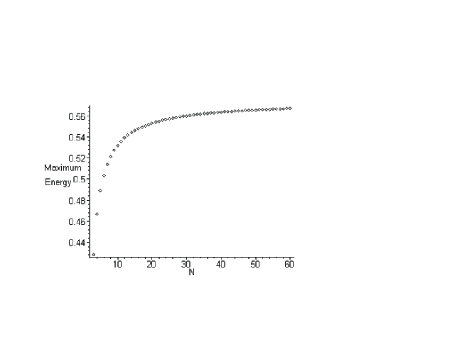
Figure 1: Maximum value of the average relativistic energy as a function of $N$.

The curve asymptotes to the constant value of $\left\langle\zeta\right\rangle=.573940872$ as $N\rightarrow\infty$.

Of course the relativistic expansion (44) breaks down well before $\beta$ reaches this point.  In figure 2 we plot the average energy $\left\langle\zeta\right\rangle$ as a function of $kT$ for $N=10$.  The relativistic case is clearly distinguishable from its non-relativistic counterpart once $kT/Mc^{2}>.02$.

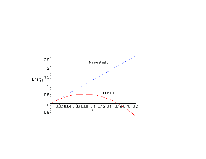
Figure 2: Average Energy $\left\langle\zeta\right\rangle$as a function of $kT$ for $N=10$ for the non-relativistic and relativistic cases. Axes are in units of $Mc^{2}$.

However the upper bound on the thermal energy is $kT/Mc^{2}<.0117$ for $N=10$. In 3 we plot the average energy over the allowed range of $kT$

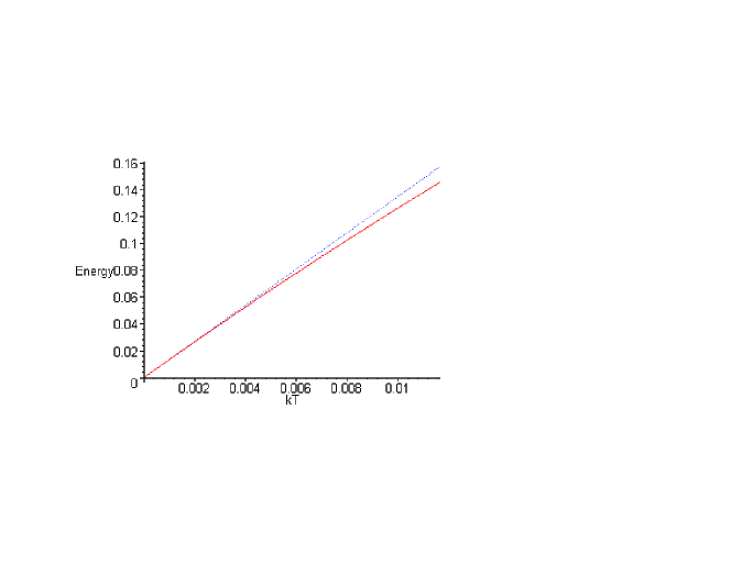
Figure 3: Average energy $\left\langle\zeta\right\rangle$ for $N=10$ over the allowed range of $kT$.

illustrating that the distinction between the two cases is about $8\%$ at most.  For $N=1000$ the maximum difference between the two cases is less than one part in a thousand over the allowed range of $\ kT$.

In the canonical case we take the energy $E$ to be the fixed total average energy as given by eq. (63).  Solving this equation for the inverse temperature $\beta$ yields

$$\beta=\frac{18\left(N-1\right)-\left[\left(5N+3\right)+\frac{8N}{\left(N-1\right)}\sum_{k=1}^{N-1}\sum_{l=k+1}^{N-1}\frac{\left(l-k\right)}{l\left(N-l\right)}\right]\zeta}{12\left(E-Mc^{2}\right)}=\frac{a_{N}}{Mc^{2}\zeta}\left(1-\frac{b_{N}}{a_{N}^{2}}\zeta\right)$$ (103)

where

$$a_{N}=\frac{3}{2}\left(N-1\right)\mbox{ \ \ \ \ \ \ \ }b_{N}=\frac{1}{8}\left(\left(5N+3\right)\left(N-1\right)+8N\sum_{k=1}^{N-1}\sum_{j=k+1}^{N-1}\frac{\left(j-k\right)}{j\left(N-k\right)}\right)$$ (104)

are defined for convenience.  The limit (100) implies that

$$1>\left(\frac{b_{N}}{a_{N}^{2}}+\frac{b_{N}}{a_{N}}\right)\zeta\equiv\frac{\zeta}{\zeta_{\max}}\longrightarrow\left(\frac{7}{4}-\frac{\pi^{2}}{9}\right)N\zeta$$ (105)

where the latter limit holds for large $N$.  Since the exponential forms a better approximation than the polynomial one, the value of $\zeta_{\max}$ is probably a bit larger than what is given in eq. (105), although it is not clear how much. We obtain

$$f_{c}^{\ast}(\eta,\xi) = \frac{M}{N}VLf^{\prime R}(mV\eta,L\xi)=\frac{2}{3N\pi G}\sqrt{\frac{4}{3}}\left(\zeta c^{2}\right)^{3/2}f^{\prime R}(mV\eta,L\xi)$$ (106)

$$= \frac{2\left(\frac{2}{3}a_{N}\right)^{3/2}}{N\sqrt{\pi\left(N-1)\right)}}\left(1-\frac{b_{N}}{a_{N}^{2}}\zeta\right)^{3/2}\exp\left[\frac{b_{N}}{a_{N}}\zeta\left(1-\frac{b_{N}}{a_{N}^{2}}\zeta\right)^{-1}\right]$$

$$\times\sum_{l=1}^{N-1}\left[\left\{A_{l}^{N}-\frac{N\zeta}{a_{N}}\left[B_{l}^{N}-A_{l}^{N}\left(1-\frac{4a_{N}}{3N}\left(1-\frac{b_{N}}{a_{N}^{2}}\zeta\right)l\left|\xi\right|\right)\right]\left(1-\frac{b_{N}}{a_{N}^{2}}\zeta\right)^{-1}\right.\right.$$

$$+A_{l}^{N}\frac{N\zeta}{2a_{N}}\left[a_{N}^{2}\frac{4\eta^{4}\left(N^{2}-3N+3\right)}{9N\left(N-1\right)^{3}}\left(1-\frac{b_{N}}{a_{N}^{2}}\zeta\right)\right]$$

$$+A_{l}^{N}\frac{N\zeta}{2a_{N}}\left[a_{N}\frac{\eta^{2}\left(N-2\right)}{N\left(N-1\right)^{2}}+\frac{3\left(N-2\right)^{2}}{4\left(N-1\right)}\left(1-\frac{b_{N}}{a_{N}^{2}}\zeta\right)^{-1}\right]$$

$$+\frac{2N\zeta}{a_{N}}\left(\frac{N}{2\left(N-1\right)}\left(1-\frac{b_{N}}{a_{N}^{2}}\zeta\right)-\frac{2a_{N}\eta^{2}}{3N}\left[\frac{N^{2}}{\left(N-1\right)^{2}}\right]\right)$$

$$\mbox{ \ \ \ \ \ \ \ \ \ \ \ \ \ \ \ \ \ \ \ \ \ \ \ \ \ }\times\left[C_{l}^{N}-\frac{1}{l}A_{l}^{N}\left(1-\frac{4a_{N}}{3N}\left(1-\frac{b_{N}}{a_{N}^{2}}\zeta\right)l\left|\xi\right|\right)\right]$$

$$\left.-\frac{N\zeta}{a_{N}}\left[D_{l}^{N}+K_{l}^{N}\left(1-\frac{4a_{N}}{3N}\left(1-\frac{b_{N}}{a_{N}^{2}}\zeta\right)l\left|\xi\right|\right)\right]\left(1-\frac{b_{N}}{a_{N}^{2}}\zeta\right)^{-1}\right\}$$

$$\left.\mbox{ \ \ \ \ \ \ \ \ \ \ \ \ \ \ \ \ \ \ \ \ }\times\exp\left(-\left(1-\frac{b_{N}}{a_{N}^{2}}\zeta\right)\left(\eta^{2}+\frac{4a_{N}}{3N}l\left|\xi\right|\right)\right)\right]$$

which is valid only to first order in $\zeta$.

The canonical density (74) becomes

$$\rho_{c}^{\ast}\left(\xi\right) = L\rho_{c}(L\xi)=\frac{2\zeta c^{2}}{3\pi GM}\rho_{c}(L\xi)$$

$$= \frac{4a_{N}}{3N}\exp\left[\frac{b_{N}}{a_{N}}\zeta\left(1-\frac{b_{N}}{a_{N}^{2}}\zeta\right)^{-1}\right]$$

$$\times\sum_{l=1}^{N-1}\left\{A_{l}^{N}\left(1-\frac{b_{N}}{a_{N}^{2}}\zeta\right)+\frac{N\zeta}{a_{N}}\left(\frac{3}{8}\frac{\left(N-1\right)^{2}}{N}A_{l}^{N}-B_{l}^{N}-D_{l}^{N}\right)\right\}$$

$$\left.+\frac{N\zeta}{a_{N}}\left[A_{l}^{N}-K_{l}^{N}\right]\left(1-\frac{4a_{N}}{3N}\left(1-\frac{b_{N}}{a_{N}^{2}}\zeta\right)l\left|\xi\right|\right)\right\}\exp\left(-2\left(1-1/N\right)\left(1-\frac{b_{N}}{a_{N}^{2}}\zeta\right)l\left|\xi\right|\right)$$

We plot in fig. 4 the non-relativistic canonical single-particle density function $\rho_{c}^{\ast}(\xi,\zeta=0)$  for various values of $N$, recovering the results of Rybicki[2]. With the exception of $N=2$, the central density grows with increasing $N$ and the distribution becomes slightly more sharply peaked.

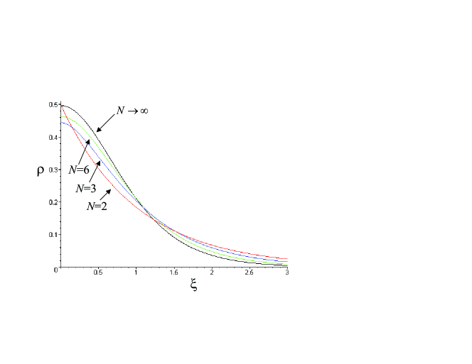
Figure 4: The non-relativistic canonical density function for various values of $N$.

It can be shown that as $N\rightarrow\infty$ the canonical density $\rho_{c}^{\ast}(\xi,\zeta=0)\rightarrow\frac{1}{2}\sec$h${}^{2}\xi$, and the single particle distribution function approaches the isothermal solution of the Vlasov equation [2].

In figs.  5 – 8 we plot the relativistic canonical function $\rho_{c}^{\ast}(\xi;\zeta)$ for differing values of $N$. As is clear from these figures, relativistic effects significantly enhance the central density by as much as 30% depending on the magnitude of $\zeta$. Even for $\zeta=0.3$, the central density is larger than its value of $1/2$ in the non-relativistic large $N$ limit. The falloff of the relativistic density functions is also more rapid than in the non-relativistic case.

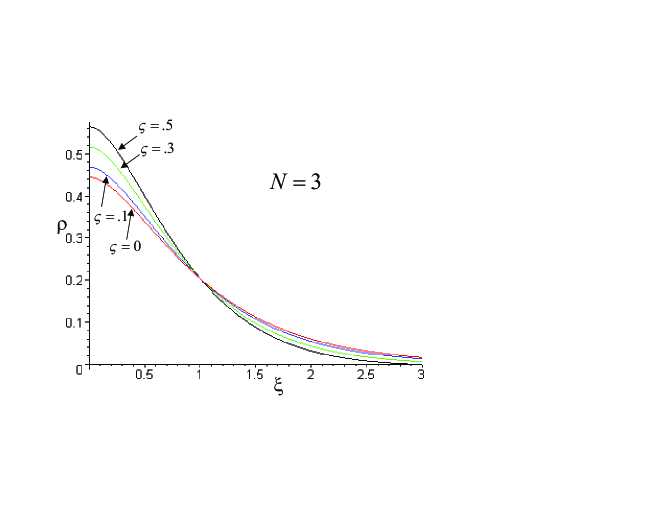
Figure 5: The canonical density function for $N=3$ for various values of the relativistic paramter $\zeta$.  The non-relativistic red curve has $\zeta=0$, and the blue, green and black curves are respectively $\zeta=0.1$, $\zeta=0.3$, and $\zeta=0.5$.  Here eq. (105)    yields $\zeta_{\max}\approx 0.43$ as the limit for which the relativistic expression is valid.

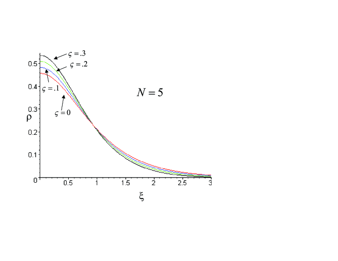
Figure 6: The canonical density function for $N=5$ where the red blue, green and black curves respectively correspond to $\zeta=0$, $0.1$, $0.2$, $0.3$, and  $\zeta_{\max}\approx 0.29$.

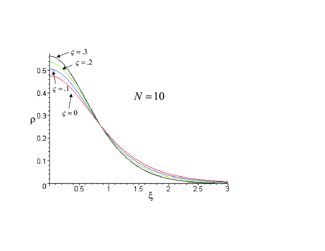
Figure 7: The canonical density function for $N=10$ where the red blue, green and black curves respectively correspond to $\zeta=0$, $0.1$, $0.2$, $0.3$, and  $\zeta_{\max}\approx 0.15$.

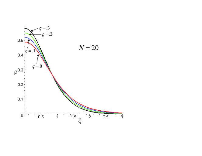
Figure 8: The canonical density function for $N=20$ where the red blue, green and black curves respectively correspond to $\zeta=0$, $0.1$, $0.2$, $0.3$, and $\zeta_{\max}\approx 0.15$.

Unfortunately there is no closed-form expression for the terms $K_{l}^{N}$ and $D_{l}^{N}$  and so it is not possible to evaluate an explicit expression for either $\ \rho_{c}^{\ast}\left(\xi\right)$ or $\rho_{mc}^{\ast}\left(\xi\right)$ in the large $N$  limit.  Instead these quantities must be computed using symbolic algebra; for $N>20$ this involve the factorization of thousands of terms, and computer memory limitations make this a prohibitive task. However the large $N$ behaviour should not be too different from the $N=20$ case, at least for small values of $\zeta$.  Figures 9 and 10 plot the density for different $N$ at two different values of $\zeta$.

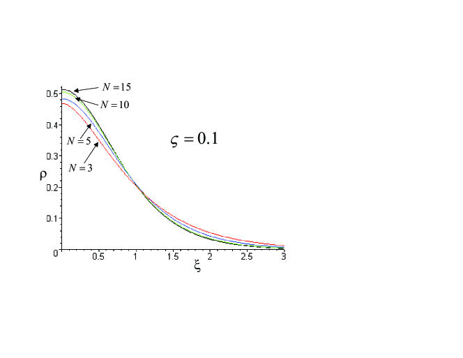
Figure 9: The canonical density for different values of $N$ at $\zeta=0.1$

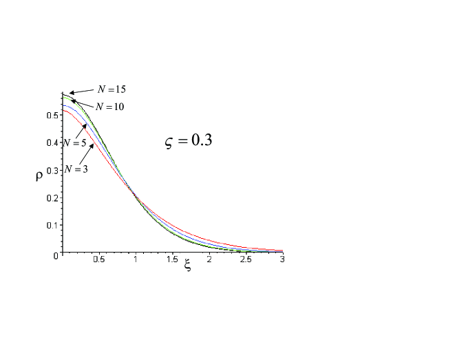
Figure 10: The canonical density for different values of $N$ at $\zeta=0.3$

The canonical momentum distribution function (75) is straightforwardly evaluated to be

$$\vartheta_{cn}^{\ast}(\eta) = mV\vartheta_{cn}(\sigma V\eta)=m\sqrt{\frac{4\zeta c^{2}}{3}}\vartheta_{cn}(\sigma V\eta)$$ (108)

$$= \frac{1}{\sqrt{\pi}}\left(1-\frac{b_{N}}{a_{N}^{2}}\zeta\right)^{1/2}\exp\left[-\eta^{2}\left(1-\frac{b_{N}}{a_{N}^{2}}\zeta\right)\right]\left(1+\frac{N\zeta}{a_{N}}\frac{\left(N^{2}-3N+3\right)}{2N\left(N-1\right)}\left(1-\frac{b_{N}}{a_{N}^{2}}\zeta\right)\eta^{4}\right.$$

$$\times\left.\frac{N\zeta}{a_{N}}\left(-\frac{\eta^{2}\left(4N^{2}-7N+6\right)}{2N\left(N-1\right)}+\frac{5N(N-1)+3}{8N\left(N-1\right)}\left(1-\frac{b_{N}}{a_{N}^{2}}\zeta\right)^{-1}\right)\right)$$

where each of (6,108) are also valid to first order in $\zeta$. Here we can easily take the large $N$ limit, which is

$$\vartheta_{c}^{\ast}(\eta)\rightarrow\frac{1}{\sqrt{\pi}}(1+\frac{\zeta}{54}(18\eta^{4}-9\eta^{2}-9-2\pi^{2}\left(2\eta^{2}-1\right))e^{-\eta^{2}}$$ (109)

to leading order in $\zeta$.

We plot in figs. 11 – 13 the behaviour of the canonical momentum density as a function of the rescaled momentum $\eta$ for differing values of $N.$ The central momentum density increases with increasing $\zeta$, and falls off more rapidly than in the non-relativistic case.

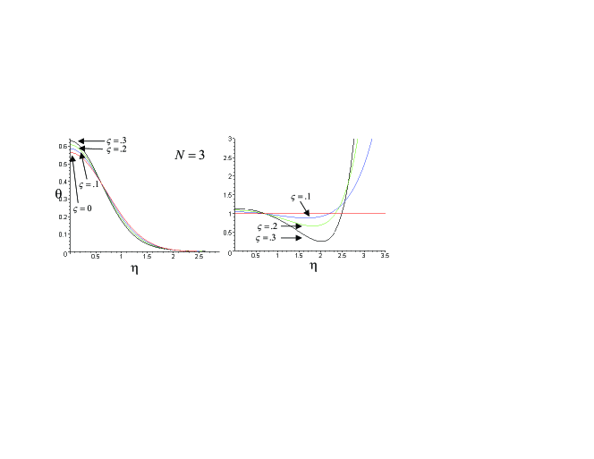
Figure 11: The canonical momentum density as a function of $\eta$ for $N=3.$ On the left hand side is the behaviour of $\ \theta_{c}^{\ast}\left(\eta;\zeta\right)$ and on the right hand side is its behaviour relative to the non-relativistic density $\theta_{c}^{\ast}\left(\eta;0\right)$. The curves are respectively red, blue, green and black for $\zeta=0,0.1,0.2,0.3$.

However for $\eta>2$, the momentum density grows relative to its non-relativistic counterpart, overtaking this value for large enough $\eta$ . The relative growth is exponential, although the overall momentum density is exponentially damped for any $\zeta$.

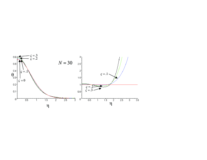
Figure 12: The canonical momentum density as a function of $\eta$ for $N=30.$ Notation is as in fig 11.

As $N$ increases, the differences between the non-relativistic and relativistic cases become less pronounced, although the basic features remain the same even in the limit that $N\rightarrow\infty$.

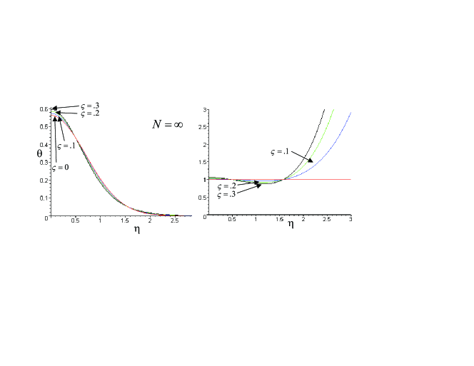
Figure 13: The canonical momentum density as a function of $\eta$ for $N=\infty.$ Notation is as in fig 11.

The microcanonical results are

$$f_{mc}^{\prime\ast R}(\eta,\xi)$$ (110)

$$= \frac{2}{3N\pi G}\sqrt{\frac{4}{3}}\left(\zeta c^{2}\right)^{3/2}f^{\prime R}(mV\eta,L\xi)$$

$$= \frac{2}{3N}\sqrt{\frac{2}{3\pi\left(N-1\right)}}\frac{\Gamma\left(\frac{3}{2}\left(N-1\right)\right)}{\Gamma\left(\frac{3}{2}\left(N-2\right)\right)}\exp\left[\frac{b_{N}}{a_{N}}\zeta\right]\sum_{l=1}^{N-1}\left\{A_{l}^{N}\left(1-\frac{2\eta^{2}}{3\left(N-1\right)}-\frac{4l\left|\xi\right|}{3N}\right)_{+}^{3N/2-4}\right.$$

$$+\zeta\eta^{2}\left(A_{l}^{N}\left[\frac{\left(N-2\right)}{\left(N-1\right)^{2}}\right]-\left(C_{l}^{N}-\frac{1}{l}A_{l}^{N}\right)\left[\frac{4N^{2}}{3\left(N-1\right)^{2}}\right]\right)\left(1-\frac{2\eta^{2}}{3\left(N-1\right)}-\frac{4l\left|\xi\right|}{3N}\right)_{+}^{3N/2-4}$$

$$+\left(\frac{3}{2}N-4\right)\zeta A_{l}^{N}\left[\frac{2\eta^{4}\left(N^{2}-3N+3\right)}{9\left(N-1\right)^{3}}-\frac{16N\left|\xi\right|\eta^{2}}{9\left(N-1\right)^{2}}\right]\left(1-\frac{2\eta^{2}}{3\left(N-1\right)}-\frac{4l\left|\xi\right|}{3N}\right)_{+}^{3N/2-5}$$

$$+\left[\frac{4\zeta}{3}\left|\xi\right|\left(A_{l}^{N}\left(\frac{N}{\left(N-1\right)}-l\right)+lK_{l}^{N}\right)\right]\left(1-\frac{2\eta^{2}}{3\left(N-1\right)}-\frac{4l\left|\xi\right|}{3N}\right)_{+}^{3N/2-4}$$

$$+\frac{N\zeta}{\left(\frac{3}{2}N-3\right)}\left(A_{l}^{N}\left[\frac{3\left(N-2\right)^{2}}{8\left(N-1\right)}+1\right]-B_{l}^{N}\mbox{\ }+\frac{N\left(C_{l}^{N}-\frac{1}{l}A_{l}^{N}\right)}{\left(N-1\right)}-D_{l}^{N}-K_{l}^{N}\right)$$

$$\mbox{ \ \ \ \ \ \ \ \ \ \ \ \ \ \ \ \ \ \ \ \ \ \ \ \ \ \ \ \ \ \ \ \ \ \ \ }\left.\times\left(1-\frac{2\eta^{2}}{3\left(N-1\right)}-\frac{4l\left|\xi\right|}{3N}\right)_{+}^{3N/2-3}\right\}$$

$$\rho_{mc}^{\ast}(\xi) \equiv L\rho_{mc}(L\xi)$$ (111)

$$= 2\exp\left[\frac{b_{N}}{a_{N}}\zeta\right]\sum_{l=1}^{N-1}\left\{\left(\frac{3N-5}{3N}\right)\left[A_{l}^{N}-\frac{4l\left|\xi\right|}{3}\zeta\left(A_{l}^{N}-K_{l}^{N}\right)\right]\left(1-\frac{4l\left|\xi\right|}{3N}\right)_{+}^{3N/2-7/2}\right.$$

$$\left.+\frac{2}{3}\zeta\left(1-\frac{4l\left|\xi\right|}{3N}\right)_{+}^{3N/2-5/2}\left(\left(\frac{3(N-1)^{2}}{8N}\right)A_{l}^{N}-\left(B_{l}^{N}-A_{l}^{N}\right)-\left(D_{l}^{N}+K_{l}^{N}\right)\right)\right\}\mbox{ \ \ \ \ \ \ \ \ \ \ \ \ }$$

and

$$\vartheta_{mc}^{\ast}(\eta) \equiv mV\vartheta_{mc}(mV\eta)$$

$$= \sqrt{\frac{2}{3\pi\left(N-1\right)}}\frac{\Gamma\left(\frac{3}{2}\left(N-1\right)\right)}{\Gamma\left(\frac{3}{2}N-2\right)}\exp\left[\frac{b_{N}}{a_{N}}\zeta\right]$$

$$\times\left\{\left[1-\left(\frac{\eta^{2}}{3}\left[\frac{8N^{2}-11N+6}{\left(N-1\right)^{2}}\right]\right)\zeta\right]\left(1-\frac{2\eta^{2}}{3\left(N-1\right)}\right)_{+}^{3N/2-3}\right.$$

$$\mbox{ \ \ \ \ \ \ \ \ \ \ \ }+\frac{\zeta\left(N-2\right)}{3}\left[\frac{\eta^{4}\left(N^{2}-3N+3\right)}{\left(N-1\right)^{3}}\right]\left(1-\frac{2\eta^{2}}{3\left(N-1\right)}\right)_{+}^{3N/2-4}$$

$$\mbox{\ }\left.-\frac{2N\zeta}{\left(3N-4\right)}\left(\frac{\left(5N^{2}-20N+12\right)}{8\left(N-1\right)}\mbox{\ }+\sum_{s=1}^{N-1}\sum_{t=s+1}^{N-1}\frac{\left(t-s\right)}{t\left(N-s\right)}\right)\left(1-\frac{2\eta^{2}}{3\left(N-1\right)}\right)_{+}^{3N/2-2}\right\}$$

where each of (110,111,6) are valid to first order in $\zeta$.  As $N\rightarrow\infty$ we have

$$\vartheta_{mc}^{\ast}(\eta)\rightarrow\frac{1}{\sqrt{\pi}}(1+\frac{\zeta}{54}(18\eta^{4}-81\eta^{2}+27-2\pi^{2}\left(2\eta^{2}-1\right))e^{-\eta^{2}}$$ (113)

Note that this differs from the canonical momentum density unless $\zeta=0.$

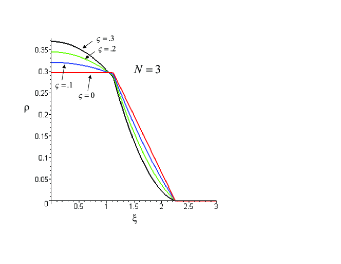
Figure 14: The microcanonical density function for $N=3$ for various values of the relativistic paramter $\zeta$.  The non-relativistic red curve has $\zeta=0$, and the blue, green and black curves are respectively $\zeta=0.1$, $\zeta=0.2$, and $\zeta=0.3$.

The microcanonical density function $\rho_{mc}^{\ast}(\xi;\zeta)$ for differing values of $N$ is plotted in figs 14–17. For $N=3$, the microcanonical density is uniform until $\xi=9/8$, after which it falls linearly to zero.  For $\xi<9/8$, at most two particles can contribute to the density; in this region relativistic effects enhance their contribution.  However for $\xi>9/8$, at most one particle can contribute, and relativistic effects suppress its contribution until $\xi=9/4$, after which the density vanishes.

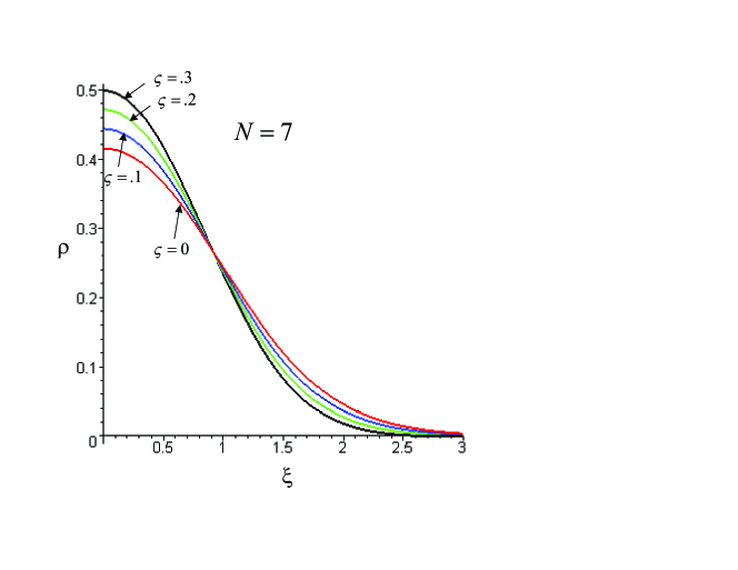
Figure 15: The microcanonical density function for $N=7$ for various values of the relativistic paramter $\zeta$. Notation is as in fig. 14.

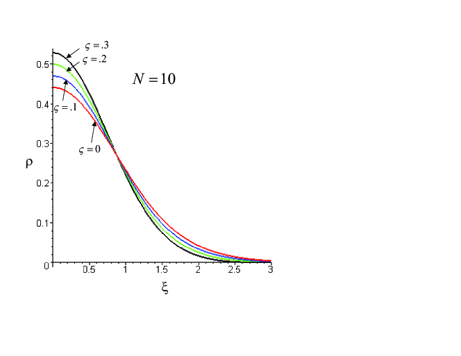
Figure 16: The microcanonical density function for $N=10$ for various values of the relativistic paramter $\zeta$. Notation is as in fig. 14.

For larger $N$, as in the canonical case, relativistic effects significantly enhance the central density by as much as 30%, depending on the size of $\zeta$.  Their falloff is more rapid, and for sufficiently large $\xi$ the non-relativistic density distribution is larger.  As $N$ increases, the density becomes more sharply peaked and the contrasts between the non-relativistic and relativistic cases become less pronounced.

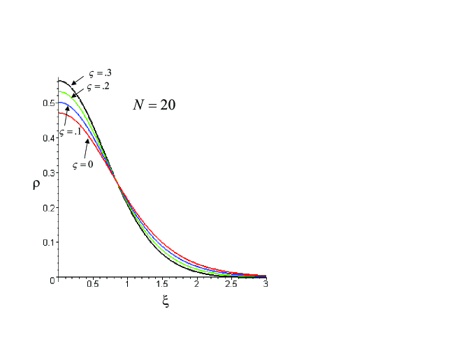
Figure 17: The microcanonical density function for $N=20$ for various values of the relativistic paramter $\zeta$. Notation is as in fig. 14.

In figs. 18, 19 we plot the microcanonical density distribution for increasing values of $N$ and fixed $\zeta$.

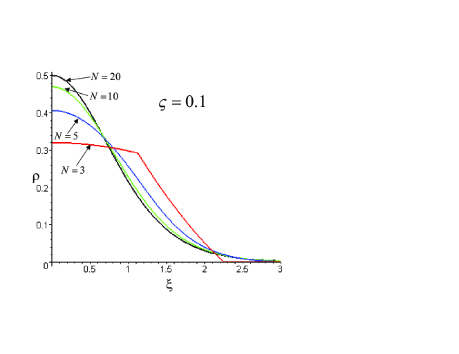
Figure 18: The microcanonical density for different values of $N$ at $\zeta=0.1$

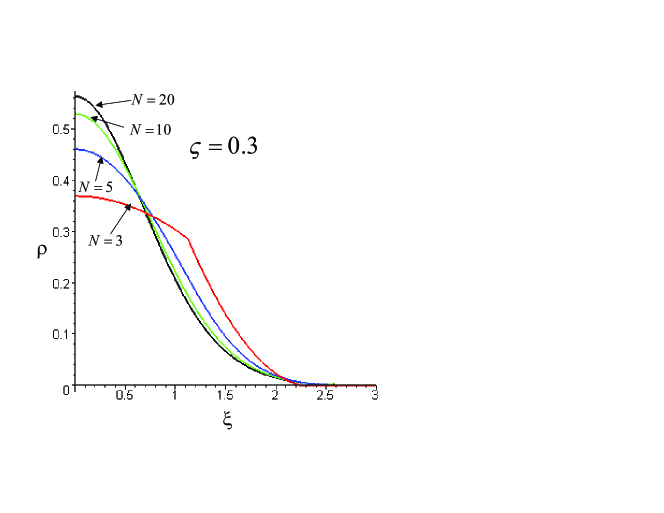
Figure 19: The microcanonical density for different values of $N$ at $\zeta=0.3$

We plot the microcanonical momentum distributions in figs. 20–22. The results are qualitatively similar to the canonical case, although the actual functional forms differ.

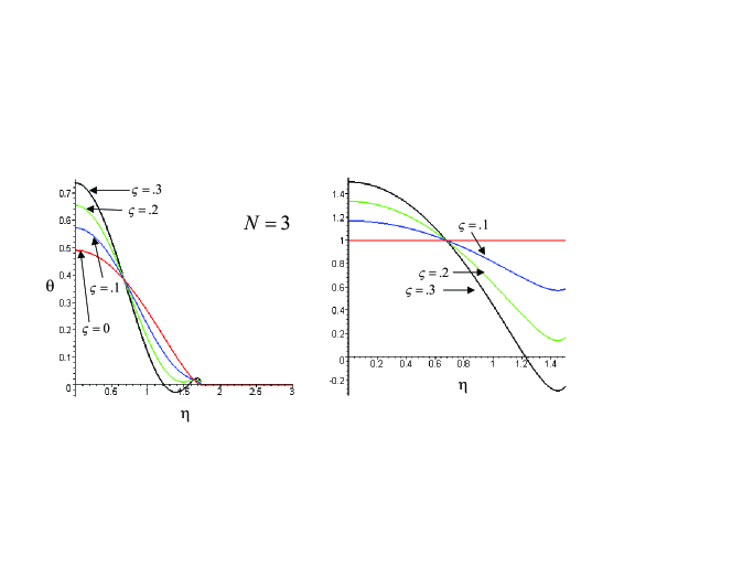
Figure 20: The microcanonical momentum density as a function of $\eta$ for $N=3.$ On the left hand side is the behaviour of $\ \theta_{mc}^{\ast}\left(\eta;\zeta\right)$ and on the right hand side is its behaviour relative to the non-relativistic density $\theta_{c}^{\ast}\left(\eta;0\right)$. The curves are respectively red, blue, green and black for $\zeta=0,0.1,0.2,0.3$.

For small $N$, the relativistic approximation breaks down even for $\zeta$ as small as $0.3$, and the momentum distribution function goes negative, as shown in fig.20.

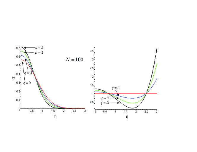
Figure 21: The microcanonical momentum density as a function of $\eta$ for $N=100$. Notation is as in fig. 20

However for larger $N$ the momentum distribution is positive for all $\zeta$ $\leq 0.3$, for example as in fig. 21.  The relativistic densities are more sharply peaked and for sufficiently large momentum parameter $\eta$ are larger than their non-relativistic counterparts.

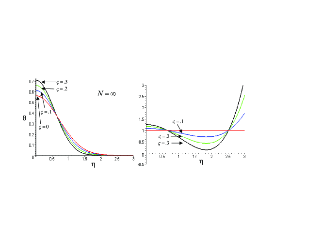
Figure 22: The microcanonical momentum density as a function of $\eta$ for $N=\infty$. Notation is as in fig. 20

7 Closing Remarks

We have carried out the first analysis of the statistical behaviour of a ROGS to leading order in $1/c$.  The qualitative behaviour of the ROGS as compared to its non-relativistic OGS counterpart [2] is clear.  At a given energy, the ROGS temperature is smaller than the OGS temperature; relativistic effects cool the gas down. The one-particle distribution functions become more sharply peaked in each case with increasing $N$.  For a given $N$, the ROGS density functions become more sharply peaked as the relativistic parameter $\zeta$ increases. For both canonical and microcanonical distribution functions, $\rho_{\mbox{OGS}}>\rho_{\mbox{ROGS}}$ for sufficiently large position parameter $\xi$. However for the momentum densities, this is not true. Although $\vartheta_{\mbox{OGS}}>\vartheta_{\mbox{ROGS}}$ for intermediate values of the momentum parameter $\eta$, once $\eta$ becomes large enough this inequality is reversed.  This behaviour is presumably due to quadratic character of the ROGS potential relative to its linear OGS counterpart in the former case, and from the $\ p^{4}$ corrections in the Hamiltonian (46) in the latter situation.

This work can be extended in several directions.  It would be straightforward to extend these results to the charged and cosmological systems considered in refs. [7, 8] to see what effects these impose on the distribution functions. Extensions to unequal masses would also be interesting, although considerably more difficult. It would be very interesting to go beyond leading order in $1/c$ to investigate non-perturbative effects of the ROGS.

Further understanding the ROGS will undoubtedly require numerical experiments for various values of $N$.  The equations of motion yield quartic (as opposed to quadratic) time-dependence of the position variables (to leading order in $1/c$), and so can be straightforwardly (although somewhat tediously) integrated to investigate its equilibrium and equipartion properties. Work on this is in progress.

Acknowledgements

This work was supported by the Natural Sciences and Engineering Research Council of Canada. We would like to thank T. Ohta for interesting discussion and correspondence.

8 Appendix

8.1 The Gaussian integrations

The following Gaussian integrations were used to obtain (51)

$$\int\frac{dk}{2\pi}\int d{\bf p}\exp\left(ik\sum_{a=1}^{N}p_{a}-\beta\sum_{a=1}^{N}\frac{p_{a}^{2}}{2m}\right)$$ (114)

$$= \int\frac{dk}{2\pi}\prod_{a=1}^{N}\int dp_{a}e^{-\beta\frac{p_{a}^{2}}{2m}+ikp_{a}}=\left(\frac{2m}{\beta}\right)^{N/2}\left(\frac{2m}{\beta}\right)^{-1/2}\int\frac{d\tilde{k}}{2\pi}\prod_{a=1}^{N}\int d\tilde{p}_{a}e^{-\tilde{p}_{a}^{2}+i\tilde{k}\tilde{p}_{a}}$$

$$= \left(\frac{2m}{\beta}\right)^{\left(N-1\right)/2}\pi^{N/2}\int\frac{d\tilde{k}}{2\pi}\exp\left(-\frac{N\tilde{k}^{2}}{4}\right)=\frac{1}{\sqrt{N}}\left(\frac{2\pi m}{\beta}\right)^{\left(N-1\right)/2}$$

$$\int\frac{dk}{2\pi}\int d{\bf p\,}p_{a}^{2}\exp\left(ik\sum_{b=1}^{N}p_{b}-\beta\sum_{b=1}^{N}\frac{p_{b}^{2}}{2m}\right)$$ (115)

$$= \left(\frac{2m}{\beta}\right)^{(N+2)/2}\left(\frac{2m}{\beta}\right)^{-1/2}\int\frac{d\tilde{k}}{2\pi}\int d\tilde{p}_{a{\bf\,}}\tilde{p}_{a}^{2}e^{-\tilde{p}_{a}^{2}+i\tilde{k}\tilde{p}_{a}}\prod_{b\neq a}^{N}\int d\tilde{p}_{b}e^{-\tilde{p}_{b}^{2}+i\tilde{k}\tilde{p}_{b}}$$

$$= \left(\frac{2m}{\beta}\right)^{(N+1)/2}\pi^{N/2}\int\frac{d\tilde{k}}{2\pi}\exp\left(-\frac{N\tilde{k}^{2}}{4}\right)\frac{1}{4}\left(2-\tilde{k}^{2}\right)$$

$$= \pi^{N/2}\left(\frac{2m}{\beta}\right)^{\left(N+1\right)/2}\frac{N-1}{2\sqrt{\pi}N^{3/2}}=\frac{N-1}{2\pi N^{3/2}}\left(\frac{2\pi m}{\beta}\right)^{\left(N+1\right)/2}$$

$$\int\frac{dk}{2\pi}\int d{\bf p\,}p_{b}p_{c}\exp\left(ik\sum_{a=1}^{N}p_{a}-\beta\sum_{a=1}^{N}\frac{p_{a}^{2}}{2m}\right)$$ (116)

$$= \left(\frac{2m}{\beta}\right)^{(N+2)/2}\left(\frac{2m}{\beta}\right)^{-1/2}\int\frac{d\tilde{k}}{2\pi}\int d\tilde{p}_{b}\tilde{p}_{b}e^{-\tilde{p}_{b}^{2}+i\tilde{k}\tilde{p}_{b}}\int d\tilde{p}_{c}\tilde{p}_{c}e^{-\tilde{p}_{c}^{2}+i\tilde{k}\tilde{p}_{c}}\prod_{a\neq b,c}^{N}\int d\tilde{p}_{a{\bf\,}}\tilde{p}_{a}^{2}e^{-\tilde{p}_{a}^{2}+i\tilde{k}\tilde{p}_{a}}$$

$$= \left(\frac{2m}{\beta}\right)^{(N+1)/2}\pi^{N/2}\int\frac{d\tilde{k}}{2\pi}\exp\left(-\frac{N\tilde{k}^{2}}{4}\right)\left(\frac{-\tilde{k}^{2}}{4}\right)=-\frac{1}{2\pi N^{3/2}}\left(\frac{2\pi m}{\beta}\right)^{\left(N+1\right)/2}$$

$$\int\frac{dk}{2\pi}\int d{\bf p\,}p_{b}^{4}\exp\left(ik\sum_{a=1}^{N}p_{a}-\beta\sum_{a=1}^{N}\frac{p_{a}^{2}}{2m}\right)$$ (117)

$$= \left(\frac{2m}{\beta}\right)^{(N+4)/2}\left(\frac{2m}{\beta}\right)^{-1/2}\int\frac{d\tilde{k}}{2\pi}\int d\tilde{p}_{a{\bf\,}}\tilde{p}_{a}^{4}e^{-\tilde{p}_{a}^{2}+i\tilde{k}\tilde{p}_{a}}\prod_{b\neq a}^{N}\int d\tilde{p}_{b}e^{-\tilde{p}_{b}^{2}+i\tilde{k}\tilde{p}_{b}}$$

$$= \left(\frac{2m}{\beta}\right)^{(N+3)/2}\pi^{N/2}\int\frac{d\tilde{k}}{2\pi}\exp\left(-\frac{N\tilde{k}^{2}}{4}\right)\frac{1}{16}\left(\tilde{k}^{4}-12\tilde{k}^{2}+12\right)$$

$$= \left(\frac{2m}{\beta}\right)^{(N+3)/2}\pi^{N/2}\frac{3\left(N-1\right)^{2}}{4\sqrt{\pi}N^{5/2}}=\frac{3\left(N-1\right)^{2}}{\left(2\pi\right)^{2}N^{5/2}}\left(\frac{2\pi m}{\beta}\right)^{(N+3)/2}$$

8.2 The $\theta(p,z)$ term

This term is

$$\theta_{cn}(p,{\bf z})=\int\frac{dk}{2\pi}\int d{\bf p}\exp\left(ik\sum_{a=1}^{N}p_{a}-\beta\sum_{a=1}^{N}\frac{p_{a}^{2}}{2m}\right)\left(1-\frac{\beta}{c^{2}}H_{R}\right)\delta\left(p-p_{n}\right)$$ (118)

where

$$H_{R} = -\lambda_{1}\sum_{a=1}^{N}\frac{p_{a}^{4}}{8m^{3}}+\pi G\lambda_{2}\sum_{a=1}^{N}\sum_{b=1}^{N}p_{b}^{2}\left|r_{ab}\right|-2\pi G\lambda_{3}\sum_{a>b}^{N}p_{a}p_{b}\left|r_{ab}\right|$$ (119)

$$+\lambda_{4}\left(\pi G\right)^{2}\sum_{a=1}^{N}\sum_{b=1}^{N}\sum_{c=1}^{N}m^{3}\left[\left|r_{ab}\right|\left|r_{ac}\right|-r_{ab}r_{ac}\right]$$

8.2.1
The classical and $\lambda_{4}$ part

Here we must compute

$$\int\frac{dk}{2\pi}\int d{\bf p}\exp\left(ik\sum_{a=1}^{N}p_{a}-\beta\sum_{a=1}^{N}\frac{p_{a}^{2}}{2m}\right)\delta\left(p-p_{n}\right)\left(1-\frac{\beta m^{3}}{c^{2}}\lambda_{4}\left(\pi G\right)^{2}\sum_{a=1}^{N}\sum_{b=1}^{N}\sum_{c=1}^{N}\left[\left|r_{ab}\right|\left|r_{ac}\right|-r_{ab}r_{ac}\right]\right)$$ (120)

of which the relevant part is

$$\int\frac{dk}{2\pi}\int d{\bf p}\exp\left(ik\sum_{a=1}^{N}p_{a}-\beta\sum_{a=1}^{N}\frac{p_{a}^{2}}{2m}\right)\delta\left(p-p_{n}\right)$$ (121)

$$= \int\frac{dk}{2\pi}\exp\left(ikp-\frac{\beta p^{2}}{2m}\right)\int d{\bf p}\exp\left(ik\sum_{a\neq n}^{N}p_{a}-\beta\sum_{a\neq n}^{N}\frac{p_{a}^{2}}{2m}\right)$$

$$= \left(\frac{2m}{\beta}\right)^{\left(N-2\right)/2}\pi^{\left(N-1\right)/2}\int\frac{d\tilde{k}}{2\pi}\exp\left(i\tilde{k}\tilde{p}-\tilde{p}^{2}\right)\exp\left(-\frac{\left(N-1\right)\tilde{k}^{2}}{4}\right)$$

$$= \left(\frac{2\pi m}{\beta}\right)^{\left(N-2\right)/2}\frac{1}{\sqrt{N-1}}\exp\left(-\frac{\beta p^{2}N}{2m\left(N-1\right)}\right)$$

and so

$$\int\frac{dk}{2\pi}\int d{\bf p}\exp\left(ik\sum_{a=1}^{N}p_{a}-\beta\sum_{a=1}^{N}\frac{p_{a}^{2}}{2m}\right)\delta\left(p-p_{n}\right)\left(1-\frac{\beta}{c^{2}}\lambda_{4}\left(\pi G\right)^{2}\sum_{a=1}^{N}\sum_{b=1}^{N}\sum_{c=1}^{N}m^{3}\left[\left|r_{ab}\right|\left|r_{ac}\right|-r_{ab}r_{ac}\right]\right)$$ (122)

$$= \left(\frac{2\pi m}{\beta}\right)^{\left(N-2\right)/2}\frac{1}{\sqrt{N-1}}\exp\left(-\frac{\beta p^{2}N}{2m\left(N-1\right)}\right)\left(1-\frac{4\beta\lambda_{4}m^{3}\left(\pi G\right)^{2}}{c^{2}}\sum_{k=1}^{N-1}\sum_{l=k+1}^{N-1}\left(N-l\right)\left(l-k\right)ku_{l}u_{k}\right)$$

where (57) was used.

8.3 The $\lambda_{1}$ part

Now we have

$$\int\frac{dk}{2\pi}\int d{\bf p}\exp\left(ik\sum_{a=1}^{N}p_{a}-\beta\sum_{a=1}^{N}\frac{p_{a}^{2}}{2m}\right)\delta\left(p-p_{n}\right)\left(-\frac{\beta}{c^{2}}\right)\left(-\lambda_{1}\sum_{c=1}^{N}\frac{p_{c}^{4}}{8m^{3}}\right)$$ (123)

$$= \frac{\lambda_{1}\beta}{8m^{3}c^{2}}\sum_{c=1}^{N}\int\frac{dk}{2\pi}\int d{\bf p}p_{c}^{4}\exp\left(ik\sum_{a=1}^{N}p_{a}-\beta\sum_{a=1}^{N}\frac{p_{a}^{2}}{2m}\right)\delta\left(p-p_{n}\right)$$

and

$$\int\frac{dk}{2\pi}\int d{\bf p}p_{c}^{4}\exp\left(ik\sum_{a=1}^{N}p_{a}-\beta\sum_{a=1}^{N}\frac{p_{a}^{2}}{2m}\right)\delta\left(p-p_{n}\right)$$ (126)

$$= \int\frac{dk}{2\pi}\exp\left(ikp-\frac{\beta p^{2}}{2m}\right)\int d{\bf p}\exp\left(ik\sum_{a\neq n}^{N}p_{a}-\beta\sum_{a\neq n}^{N}\frac{p_{a}^{2}}{2m}\right)\left\{\begin{array}[]{c}p_{c}^{4}\mbox{\ \ \ \ \ \ \ \ \ \ \ }\left(c\neq n\right)\\ p^{4}\mbox{\ \ \ \ \ \ \ \ \ \ \ }\left(c=n\right)\end{array}\right.$$

$$= \left(\frac{2\pi m}{\beta}\right)^{\left(N+2\right)/2}\frac{1}{\pi^{2}}\exp\left(-\frac{\beta p^{2}N}{2m\left(N-1\right)}\right)\left\{\begin{array}[]{l}\left(\frac{\beta^{2}p^{4}}{\left(2m\right)^{2}\left(N-1\right)^{9/2}}+\frac{3\left(N-2\right)\beta p^{2}}{2m\left(N-1\right)^{7/2}}+\frac{3\left(N-2\right)^{2}}{4\left(N-1\right)^{5/2}}\right)\mbox{ \ \ \ \ \ \ }\left(c\neq n\right)\\ \left(\frac{\beta^{2}p^{4}}{\left(2m\right)^{2}\left(N-1\right)^{1/2}}\right)\mbox{ \ \ \ \ \ \ \ \ \ \ \ \ \ \ \ \ }\left(c=n\right)\mbox{\ \ \ \ \ \ \ }\end{array}\right.$$ (129)

which gives

$$\int\frac{dk}{2\pi}\int d{\bf p}\exp\left(ik\sum_{a=1}^{N}p_{a}-\beta\sum_{a=1}^{N}\frac{p_{a}^{2}}{2m}\right)\delta\left(p-p_{n}\right)\left(-\frac{\beta}{c^{2}}\right)\left(-\lambda_{1}\sum_{c=1}^{N}\frac{p_{c}^{4}}{8m^{3}}\right)$$

$$= \left(\frac{2\pi m}{\beta}\right)^{\left(N+2\right)/2}\frac{\lambda_{1}\beta}{8m^{3}\pi^{2}c^{2}}\exp\left(-\frac{\beta p^{2}N}{2m\left(N-1\right)}\right)$$

$$\mbox{ \ \ \ \ }\times\left\{\left(N-1\right)\left(\frac{\beta^{2}p^{4}}{\left(2m\right)^{2}\left(N-1\right)^{9/2}}+\frac{3\left(N-2\right)\beta p^{2}}{2m\left(N-1\right)^{7/2}}+\frac{3\left(N-2\right)^{2}}{4\left(N-1\right)^{5/2}}\right)+\frac{\beta^{2}p^{4}}{\left(2m\right)^{2}\left(N-1\right)^{1/2}}\right\}$$

$$= \left(\frac{2\pi m}{\beta}\right)^{\left(N-2\right)/2}\frac{\exp\left(-\frac{\beta p^{2}N}{2m\left(N-1\right)}\right)}{\sqrt{N-1}}\frac{\lambda_{1}}{2\beta mc^{2}}\left(\frac{\beta^{2}p^{4}\left(1+\left(N-1\right)^{3}\right)}{\left(2m\right)^{2}\left(N-1\right)^{3}}+\frac{3\left(N-2\right)\beta p^{2}}{2m\left(N-1\right)^{2}}+\frac{3\left(N-2\right)^{2}}{4\left(N-1\right)}\right)$$

8.3.1 The $\lambda_{2}$ part

Now we must do

$$\int\frac{dk}{2\pi}\int d{\bf p}\exp\left(ik\sum_{a=1}^{N}p_{a}-\beta\sum_{a=1}^{N}\frac{p_{a}^{2}}{2m}\right)\delta\left(p-p_{n}\right)\left(-\frac{\beta}{c^{2}}\right)\left(+\pi G\lambda_{2}\sum_{a=1}^{N}\sum_{b=1}^{N}p_{b}^{2}\left|r_{ab}\right|\right)$$ (131)

$$= -\frac{\lambda_{2}\pi G\beta}{c^{2}}\sum_{c=1}^{N}\sum_{b=1}^{N}\left|r_{bc}\right|\int\frac{dk}{2\pi}\int d{\bf p\,}p_{b}^{2}\exp\left(ik\sum_{a=1}^{N}p_{a}-\beta\sum_{a=1}^{N}\frac{p_{a}^{2}}{2m}\right)\delta\left(p-p_{n}\right)$$

and the integrals are

$$\int\frac{dk}{2\pi}\int d{\bf p}p_{c}^{2}\exp\left(ik\sum_{a=1}^{N}p_{a}-\beta\sum_{a=1}^{N}\frac{p_{a}^{2}}{2m}\right)\delta\left(p-p_{n}\right)$$ (134)

$$= \int\frac{dk}{2\pi}\exp\left(ikp-\frac{\beta p^{2}}{2m}\right)\int d{\bf p}\exp\left(ik\sum_{a\neq n}^{N}p_{a}-\beta\sum_{a\neq n}^{N}\frac{p_{a}^{2}}{2m}\right)\left\{\begin{array}[]{c}p_{c}^{2}\mbox{\ \ \ \ \ \ \ \ \ \ \ }\left(c\neq n\right)\\ p^{2}\mbox{\ \ \ \ \ \ \ \ \ \ \ }\left(c=n\right)\end{array}\right.$$

$$= \left(\frac{2\pi m}{\beta}\right)^{N/2}\frac{1}{\pi}\exp\left(-\frac{\beta p^{2}N}{2m\left(N-1\right)}\right)\left\{\begin{array}[]{l}\left(\frac{\beta p^{2}}{2m\left(N-1\right)^{5/2}}+\frac{\left(N-2\right)}{2\left(N-1\right)^{3/2}}\right)\mbox{ \ \ \ \ \ \ }\left(c\neq n\right)\\ \left(\frac{\beta p^{2}}{2m\left(N-1\right)^{1/2}}\right)\mbox{ \ \ \ \ \ \ \ \ \ \ \ \ \ \ \ \ \ \ \ \ \ }\left(c=n\right)\mbox{\ \ \ \ \ }\end{array}\right.$$ (137)

giving

$$\int\frac{dk}{2\pi}\int d{\bf p}\exp\left(ik\sum_{a=1}^{N}p_{a}-\beta\sum_{a=1}^{N}\frac{p_{a}^{2}}{2m}\right)\delta\left(p-p_{n}\right)\left(-\frac{\beta}{c^{2}}\right)\left(+\pi G\lambda_{2}\sum_{a=1}^{N}\sum_{b=1}^{N}p_{b}^{2}\left|r_{ab}\right|\right)$$ (138)

$$= -\frac{\lambda_{2}\pi G\beta}{c^{2}}\left(\frac{2\pi m}{\beta}\right)^{N/2}\frac{1}{\pi}\exp\left(-\frac{\beta p^{2}N}{2m\left(N-1\right)}\right)$$

$$\mbox{ \ }\times\left(\sum_{c=1}^{N}\sum_{b\neq n}^{N}\left|r_{bc}\right|\left\{\frac{\beta p^{2}}{2m\left(N-1\right)^{5/2}}+\frac{\left(N-2\right)}{2\left(N-1\right)^{3/2}}\right\}+\sum_{c=1}^{N}\left|r_{cn}\right|\left(\frac{\beta p^{2}}{2m\left(N-1\right)^{1/2}}\right)\right)$$

$$= -\frac{\mbox{2}\lambda_{2}\pi Gm}{c^{2}}\frac{1}{\sqrt{N-1}}\left(\frac{2\pi m}{\beta}\right)^{\left(N-2\right)/2}\exp\left(-\frac{\beta p^{2}N}{2m\left(N-1\right)}\right)$$

$$\mbox{ \ \ \ \ \ \ \ \ \ \ }\times\left(\sum_{c=1}^{N}\sum_{b\neq n}^{N}\left|r_{bc}\right|\left\{\frac{\beta p^{2}}{2m\left(N-1\right)^{2}}+\frac{\left(N-2\right)}{2\left(N-1\right)}\right\}+\sum_{c=1}^{N}\left|r_{cn}\right|\left(+\frac{\beta p^{2}}{2m}\right)\right)$$

Since $\sum_{b\neq n}^{N}\left|r_{cb}\right|=\sum_{b=1}^{N}\left|r_{cb}\right|-\left|r_{cn}\right|$, this becomes

$$\int\frac{dk}{2\pi}\int d{\bf p}\exp\left(ik\sum_{a=1}^{N}p_{a}-\beta\sum_{a=1}^{N}\frac{p_{a}^{2}}{2m}\right)\delta\left(p-p_{n}\right)\left(-\frac{\beta}{c^{2}}\right)\left(+\pi G\lambda_{2}\sum_{a=1}^{N}\sum_{b=1}^{N}p_{b}^{2}\left|r_{ab}\right|\right)$$ (139)

$$= -\frac{\mbox{2}\lambda_{2}\pi Gm}{\sqrt{N-1}c^{2}}\left(\frac{2\pi m}{\beta}\right)^{\left(N-2\right)/2}\exp\left(-\frac{\beta p^{2}N}{2m\left(N-1\right)}\right)\left\{\sum_{c=1}^{N}\sum_{b=1}^{N}\left|r_{bc}\right|\left\{\frac{\beta p^{2}}{2m\left(N-1\right)^{2}}+\frac{\left(N-2\right)}{2\left(N-1\right)}\right\}\right.$$

$$\mbox{ \ \ \ \ \ \ \ }\left.+\sum_{c=1}^{N}\left|r_{cn}\right|\left(+\frac{\beta p^{2}}{2m}\left[\frac{N\left(N-2\right)}{\left(N-1\right)^{2}}\right]-\frac{\left(N-2\right)}{2\left(N-1\right)}\right)\right\}$$

$$= -\frac{\mbox{2}\lambda_{2}\pi Gm}{\sqrt{N-1}c^{2}}\left(\frac{2\pi m}{\beta}\right)^{\left(N-2\right)/2}\exp\left(-\frac{\beta p^{2}N}{2m\left(N-1\right)}\right)\left(2\sum_{l=1}^{N-1}l\left(N-l\right)u_{l}\left\{\frac{\beta p^{2}}{2m\left(N-1\right)^{2}}+\frac{\left(N-2\right)}{2\left(N-1\right)}\right\}\right.$$

$$\mbox{ \ \ \ \ \ \ \ \ \ \ \ \ \ \ \ \ \ \ \ \ \ \ \ \ }+\left.\left(\sum_{s=1}^{n-1}su_{s}+\sum_{s=n}^{N-1}(N-s)u_{s}\right)\left(+\frac{\beta p^{2}}{2m}\left[\frac{N\left(N-2\right)}{\left(N-1\right)^{2}}\right]-\frac{\left(N-2\right)}{2\left(N-1\right)}\right)\right)$$

8.3.2 The $\lambda_{3}$ part

Now we must do

$$\int\frac{dk}{2\pi}\int d{\bf p}\exp\left(ik\sum_{a=1}^{N}p_{a}-\beta\sum_{a=1}^{N}\frac{p_{a}^{2}}{2m}\right)\delta\left(p-p_{n}\right)\left(-\frac{\beta}{c^{2}}\right)\left(-2\pi G\lambda_{3}\sum_{a>b}^{N}p_{a}p_{b}\left|r_{ab}\right|\right)$$

$$= \frac{\lambda_{3}\pi G\beta}{c^{2}}\int\frac{dk}{2\pi}\int d{\bf p}\exp\left(ik\sum_{a=1}^{N}p_{a}-\beta\sum_{a=1}^{N}\frac{p_{a}^{2}}{2m}\right)\delta\left(p-p_{n}\right)\left(\sum_{c\neq n}^{N}\sum_{b\neq n}^{N}p_{c}p_{b}\left|r_{cb}\right|+2p\sum_{c=1}^{N}\left|r_{cn}\right|p_{c}\right)$$

where the integrations are

$$\int\frac{dk}{2\pi}\int d{\bf p}p_{b}p_{c}\exp\left(ik\sum_{a=1}^{N}p_{a}-\beta\sum_{a=1}^{N}\frac{p_{a}^{2}}{2m}\right)\delta\left(p-p_{n}\right)$$ (143)

$$= \mbox{ }\left(\frac{2\pi m}{\beta}\right)^{N/2}\frac{1}{\pi}\exp\left(-\frac{\beta p^{2}N}{2m\left(N-1\right)}\right)\left\{\begin{array}[]{l}\left(\frac{\beta p^{2}}{2m\left(N-1\right)^{5/2}}-\frac{1}{2\left(N-1\right)^{3/2}}\right)\mbox{ \ \ \ \ \ \ }\left(b\neq c\neq n\right)\\ \left(-\frac{\beta}{2m}\frac{p^{2}}{\left(N-1\right)^{3/2}}\right)\mbox{ \ \ \ \ \ \ \ \ \ \ \ \ \ \ \ \ \ \ }\left(c\neq n,b=n\right)\end{array}\right.$$

giving

$$\int\frac{dk}{2\pi}\int d{\bf p}\exp\left(ik\sum_{a=1}^{N}p_{a}-\beta\sum_{a=1}^{N}\frac{p_{a}^{2}}{2m}\right)\delta\left(p-p_{n}\right)\left(-\frac{\beta}{c^{2}}\right)\left(-2\pi G\lambda_{3}\sum_{a>b}^{N}p_{a}p_{b}\left|r_{ab}\right|\right)$$ (144)

$$= \frac{\lambda_{3}\pi G\beta}{c^{2}}\left(\frac{2\pi m}{\beta}\right)^{N/2}\frac{1}{\pi}\exp\left(-\frac{\beta p^{2}N}{2m\left(N-1\right)}\right)\left\{2\sum_{c=1}^{N}\left|r_{cn}\right|\left(-\frac{\beta}{2m}\frac{p^{2}}{\left(N-1\right)^{3/2}}\right)\right.$$

$$\mbox{ \ \ \ \ \ \ \ \ \ \ }\left.+\sum_{c\neq n}^{N}\sum_{b\neq n}^{N}\left|r_{bc}\right|\left(\frac{\beta p^{2}}{2m\left(N-1\right)^{5/2}}-\frac{1}{2\left(N-1\right)^{3/2}}\right)\right\}$$

Using again $\sum_{b\neq n}^{N}\left|r_{cb}\right|=\sum_{b=1}^{N}\left|r_{cb}\right|-\left|r_{cn}\right|$, this becomes

$$\int\frac{dk}{2\pi}\int d{\bf p}\exp\left(ik\sum_{a=1}^{N}p_{a}-\beta\sum_{a=1}^{N}\frac{p_{a}^{2}}{2m}\right)\delta\left(p-p_{n}\right)\left(-\frac{\beta}{c^{2}}\right)\left(-2\pi G\lambda_{3}\sum_{a>b}^{N}p_{a}p_{b}\left|r_{ab}\right|\right)$$

$$= \frac{\lambda_{3}\pi G\beta}{c^{2}}\left(\frac{2\pi m}{\beta}\right)^{N/2}\frac{1}{\pi}\exp\left(-\frac{\beta p^{2}N}{2m\left(N-1\right)}\right)\left\{2\sum_{c=1}^{N}\left|r_{cn}\right|\left(-\frac{\beta}{2m}\frac{p^{2}}{\left(N-1\right)^{3/2}}\right)\right.$$

$$\mbox{ \ \ \ \ \ \ \ \ \ \ \ \ \ \ \ \ \ \ \ \ \ \ \ \ \ \ }\left.+\left(\sum_{c=1}^{N}\sum_{b=1}^{N}\left|r_{bc}\right|-2\sum_{c=1}^{N}\left|r_{cn}\right|\right)\left(\frac{\beta p^{2}}{2m\left(N-1\right)^{5/2}}-\frac{1}{2\left(N-1\right)^{3/2}}\right)\right\}$$

$$= \frac{\mbox{2}\lambda_{3}\pi Gm}{\sqrt{N-1}c^{2}}\left(\frac{2\pi m}{\beta}\right)^{\left(N-2\right)/2}\exp\left(-\frac{\beta p^{2}N}{2m\left(N-1\right)}\right)\left\{\sum_{c=1}^{N}\sum_{b=1}^{N}\left|r_{bc}\right|\left(\frac{\beta p^{2}}{2m\left(N-1\right)^{2}}-\frac{1}{2\left(N-1\right)}\right)\right.$$

$$\mbox{ \ \ \ \ \ \ \ \ \ \ \ \ \ \ \ \ \ \ \ \ }\left.+\sum_{c=1}^{N}\left|r_{cn}\right|\left(\frac{1}{\left(N-1\right)}-\frac{\beta p^{2}}{2m}\left[\frac{2N}{\left(N-1\right)^{2}}\right]\right)\right\}$$

$$= \frac{\mbox{2}\lambda_{3}\pi Gm}{\sqrt{N-1}c^{2}}\left(\frac{2\pi m}{\beta}\right)^{\left(N-2\right)/2}\exp\left(-\frac{\beta p^{2}N}{2m\left(N-1\right)}\right)\left(2\sum_{l=1}^{N-1}l\left(N-l\right)u_{l}\left(\frac{\beta p^{2}}{2m\left(N-1\right)^{2}}-\frac{1}{2\left(N-1\right)}\right)\right.$$

$$\mbox{ \ \ \ \ \ \ \ \ \ \ \ \ \ \ \ \ \ \ \ \ }\left.+\left(\sum_{s=1}^{n-1}su_{s}+\sum_{s=n}^{N-1}(N-s)u_{s}\right)\left(\frac{1}{\left(N-1\right)}-\frac{\beta p^{2}}{2m}\left[\frac{2N}{\left(N-1\right)^{2}}\right]\right)\right)$$

8.3.3
The full expression for $\theta_{cn}(p,{\bf z})$

From eqs. (122,LABEL:appl1C,139,LABEL:appl3D) we have

$$\theta_{cn}(p,{\bf z}) = \int\frac{dk}{2\pi}\int d{\bf p}\exp\left(ik\sum_{a=1}^{N}p_{a}-\beta\sum_{a=1}^{N}\frac{p_{a}^{2}}{2m}\right)\left(1-\frac{\beta}{c^{2}}H_{R}\right)\delta\left(p-p_{n}\right)$$ (146)

$$= \left(\frac{2\pi m}{\beta}\right)^{\left(N-2\right)/2}\frac{1}{\sqrt{N-1}}\exp\left(-\frac{\beta p^{2}N}{2m\left(N-1\right)}\right)$$

$$\times\left(1+\frac{\lambda_{1}}{2\beta mc^{2}}\left(\frac{\beta^{2}p^{4}\left(1+\left(N-1\right)^{3}\right)}{\left(2m\right)^{2}\left(N-1\right)^{3}}+\frac{3\left(N-2\right)\beta p^{2}}{2m\left(N-1\right)^{2}}+\frac{3\left(N-2\right)^{2}}{4\left(N-1\right)}\right)\right.$$

$$\mbox{ \ \ }+\frac{\mbox{2}\lambda_{2}\pi Gm}{c^{2}}\left[-2\sum_{l=1}^{N-1}l\left(N-l\right)u_{l}\left\{\frac{\beta p^{2}}{2m\left(N-1\right)^{2}}+\frac{\left(N-2\right)}{2\left(N-1\right)}\right\}\right.$$

$$\mbox{ \ \ \ \ \ \ \ \ \ \ \ \ \ \ \ \ \ }\left.+\left(\sum_{s=1}^{n-1}su_{s}+\sum_{s=n}^{N-1}(N-s)u_{s}\right)\left(\frac{\left(N-2\right)}{2\left(N-1\right)}-\frac{\beta p^{2}}{2m}\left[\frac{N\left(N-2\right)}{\left(N-1\right)^{2}}\right]\right)\right]$$

$$\mbox{ \ \ }+\frac{\mbox{2}\lambda_{3}\pi Gm}{c^{2}}\left[2\sum_{l=1}^{N-1}l\left(N-l\right)u_{l}\left(\frac{\beta p^{2}}{2m\left(N-1\right)^{2}}-\frac{1}{2\left(N-1\right)}\right)\right.$$

$$\mbox{ \ \ \ \ \ \ \ \ \ \ \ \ \ \ \ }\left.+\left(\sum_{s=1}^{n-1}su_{s}+\sum_{s=n}^{N-1}(N-s)u_{s}\right)\left(\frac{1}{\left(N-1\right)}-\frac{\beta p^{2}}{2m}\left[\frac{2N}{\left(N-1\right)^{2}}\right]\right)\right]$$

$$\mbox{ \ \ \ }\left.-\frac{4\beta m^{3}}{c^{2}}\lambda_{4}\left(\pi G\right)^{2}\sum_{k=1}^{N-1}\sum_{l=k+1}^{N-1}\left(N-l\right)\left(l-k\right)ku_{l}u_{k}\right)$$

or alternatively

$$\theta_{cn}(p,{\bf z}) = \left(\frac{2\pi m}{\beta}\right)^{\left(N-2\right)/2}\frac{1}{\sqrt{N-1}}\exp\left(-\frac{\beta p^{2}N}{2m\left(N-1\right)}\right)$$ (147)

$$\mbox{ \ \ }\times\left[1+\frac{\lambda_{1}}{2\beta mc^{2}}\left(\frac{\beta^{2}p^{4}\left(1+\left(N-1\right)^{3}\right)}{\left(2m\right)^{2}\left(N-1\right)^{3}}+\frac{3\left(N-2\right)\beta p^{2}}{2m\left(N-1\right)^{2}}+\frac{3\left(N-2\right)^{2}}{4\left(N-1\right)}\right)\right.$$

$$\mbox{ \ \ \ \ }-\frac{4\beta m}{c^{2}}\lambda_{4}\left(\pi Gm\right)^{2}\sum_{k=1}^{N-1}\sum_{l=k+1}^{N-1}\left(N-l\right)\left(l-k\right)ku_{l}u_{k}$$

$$\mbox{ \ \ \ \ \ \ \ \ \ }+\frac{\mbox{2}\pi Gm}{c^{2}}\sum_{l=1}^{N-1}l\left(N-l\right)u_{l}\left(\frac{\left(2\lambda_{3}-2\lambda_{2}\right)\beta p^{2}}{2m\left(N-1\right)^{2}}-\frac{\left(2\lambda_{3}+2(N-2)\lambda_{2}\right)}{2\left(N-1\right)}\right)$$

$$\mbox{ \ \ \ \ \ \ \ \ \ \ }\left.+\frac{\mbox{2}\left(2\lambda_{3}+(N-2)\lambda_{2}\right)\pi Gm}{c^{2}}\left(\sum_{s=1}^{n-1}su_{s}+\sum_{s=n}^{N-1}(N-s)u_{s}\right)\left(\frac{N-1-\frac{N\beta p^{2}}{m}}{2\left(N-1\right)^{2}}\right)\right]$$

When the $\lambda$’s are all equal to unity, this is

$$\theta_{cn}(p,{\bf u}) = \frac{1}{\sqrt{N-1}}\exp\left(-\frac{N\beta p^{2}}{2m\left(N-1\right)}\right)\left(\frac{2\pi m}{\beta}\right)^{\left(N-2\right)/2}$$

$$\times\left\{\left(1-\frac{4\beta m\left(\pi Gm\right)^{2}}{c^{2}}\sum_{k=1}^{N-1}\sum_{l=k+1}^{N-1}\left(N-l\right)\left(l-k\right)ku_{l}u_{k}\right)\right.$$

$$+\frac{1}{2\beta mc^{2}}\left[\frac{\beta^{2}p^{4}N\left(N^{2}-3N+3\right)}{(2m)^{2}\left(N-1\right)^{3}}+\frac{3\beta p^{2}\left(N-2\right)}{2m\left(N-1\right)^{5/2}}+\frac{3\left(N-2\right)^{2}}{4\left(N-1\right)^{3/2}}\right]$$

$$+\left(\frac{\mbox{2}\pi mG}{c^{2}}\right)\left[-\sum_{l=1}^{N-1}l\left(N-l\right)u_{l}-\left(\frac{N^{2}\beta p^{2}}{2m\left(N-1\right)^{2}}-\frac{N}{2(N-1)}\right)\left(\sum_{s=1}^{n-1}su_{s}+\sum_{s=n}^{N-1}(N-s)u_{s}\right)\right]$$

8.4 An evaluation of $f_{cn}(p,z)$ 

Now consider eq. (LABEL:can24b), which can be rewritten as

$$f_{cn}^{R}(p,z)=\frac{e^{-\beta Mc^{2}}}{{\cal Z}}\int\frac{dk}{2\pi}\int d{\bf u}\exp\left(-ikz-\lambda\beta\sum_{l=1}^{N-1}\left(C_{l}+i\alpha D_{nl}\right)u_{l}\right)\theta_{cn}(p,{\bf u})$$ (149)

where

$$\lambda=2\pi Gm^{2}\mbox{ \ \ \ \ }\alpha=\frac{k}{N\beta\lambda}\mbox{ }$$ (150)

The integrals are now

$$I_{n}^{0} = \int d{\bf u}\exp\left(-\lambda\beta\sum_{l=1}^{N-1}\left(C_{l}+i\alpha D_{nl}\right)u_{l}\right)$$ (151)

$$= \frac{1}{\left(2\pi G\beta m^{2}\mbox{ }\right)^{N-1}}\prod_{l=1}^{N-1}\frac{1}{C_{l}+i\alpha D_{nl}}$$

$$I_{n,s}^{1} = \int d{\bf u}\exp\left(-\lambda\beta\sum_{l=1}^{N-1}\left(C_{l}+i\alpha D_{nl}\right)u_{l}\right)u_{s}$$ (152)

$$= \frac{1}{\left(2\pi G\beta m^{2}\mbox{ }\right)^{N}}\frac{1}{C_{s}+i\alpha D_{ns}}\prod_{l=1}^{N-1}\frac{1}{C_{l}+i\alpha D_{nl}}$$

$$I_{n,s,t}^{2} = \int d{\bf u}\exp\left(-\lambda\beta\sum_{l=1}^{N-1}\left(C_{l}+i\alpha D_{nl}\right)u_{l}\right)u_{s}u_{t}$$ (153)

$$= \frac{1}{\left(2\pi G\beta m^{2}\mbox{ }\right)^{N+1}}\frac{1}{C_{s}+i\alpha D_{ns}}\frac{1}{C_{t}+i\alpha D_{nt}}\prod_{l=1}^{N-1}\frac{1}{C_{l}+i\alpha D_{nl}}$$

and we must divide by $N$ and sum over all values of $n$ to obtain the correct result.

For example

$$\frac{1}{N}\sum_{n=1}^{N}I_{n}^{0} = \frac{1}{N\left(2\pi G\beta m^{2}\mbox{ }\right)^{N-1}}\sum_{n=1}^{N}\left[\prod_{l=1}^{n-1}\frac{1}{l\left(N-l-i\alpha\right)}\prod_{l=n}^{N-1}\frac{1}{\left(N-l\right)\left(l+i\alpha\right)}\right]$$ (154)

$$= \frac{1}{N\left(2\pi G\beta m^{2}\mbox{ }\right)^{N-1}}\sum_{n=1}^{N}\frac{1}{\left(n-1\right)!(N-n)!}\frac{\Gamma\left(N-n+1-i\alpha\right)}{\Gamma\left(N-i\alpha\right)}\frac{\Gamma\left(n+i\alpha\right)}{\Gamma\left(N+i\alpha\right)}$$

$$= \frac{1}{\Gamma\left(N-i\alpha\right)\Gamma\left(N+i\alpha\right)\left(2\pi G\beta m^{2}\mbox{ }\right)^{N-1}}\sum_{n=1}^{N}\frac{\left(N-1\right)!}{\left(n-1\right)!(N-n)!}\int_{0}^{1}dww^{N-n-i\alpha}\left(1-w\right)^{n+i\alpha-1}$$

$$= \frac{1}{\Gamma\left(N-i\alpha\right)\Gamma\left(N+i\alpha\right)\left(2\pi G\beta m^{2}\mbox{ }\right)^{N-1}}\int_{0}^{1}dww^{-i\alpha}\left(1-w\right)^{i\alpha}\left(w+1-w\right)^{N-1}$$

$$= \frac{1}{\left(2\pi G\beta m^{2}\mbox{ }\right)^{N-1}}\frac{\Gamma\left(1-i\alpha\right)}{\Gamma\left(N-i\alpha\right)}\frac{\Gamma\left(1+i\alpha\right)}{\Gamma\left(N+i\alpha\right)}$$

This function has single poles at $\alpha=in$, where $n$ is an integer taking its values between $-N$ and $N$, except for $N=0$. Its residues are

$$\mbox{Residue}\left[\frac{\Gamma\left(1-i\alpha\right)}{\Gamma\left(N-i\alpha\right)}\frac{\Gamma\left(1+i\alpha\right)}{\Gamma\left(N+i\alpha\right)}\right]_{a=in}=\frac{in\left(-1\right)^{n}}{\Gamma\left(N-n\right)\Gamma\left(N+n\right)}$$ (155)

yielding

$$\frac{1}{N}\sum_{n=1}^{N}\int\frac{dk}{2\pi}\int d{\bf u}\mbox{ }e^{\left(-ikz-\lambda\beta\sum_{l=1}^{N-1}\left(C_{l}+i\alpha D_{nl}\right)u_{l}\right)}=\frac{2N\beta\pi Gm^{2}}{\left(2\pi G\beta m^{2}\mbox{ }\right)^{N-1}\left[\Gamma(N)\right]^{2}}\sum_{l=1}^{N-1}A_{l}^{N}\exp\left(-2N\left(\beta\pi Gm^{2}\right)l\left|z\right|\right)$$ (156)

for the leading non-relativistic term, where

$$A_{n}^{N}=\frac{n\left(-1\right)^{n+1}\left[\Gamma(N)\right]^{2}}{\Gamma\left(N-n\right)\Gamma\left(N+n\right)}$$ (157)

The remaining integrals are somewhat more difficult. We obtain

$$\frac{1}{N}\sum_{n=1}^{N}\int d{\bf u}e^{\left(-ikz-\lambda\beta\sum_{l=1}^{N-1}\left(C_{l}+i\alpha D_{nl}\right)u_{l}\right)}\sum_{s=1}^{N-1}s\left(N-s\right)u_{s}$$ (158)

$$= -\frac{1}{\lambda\beta N}\sum_{n=1}^{N}\frac{d}{d\sigma}\left[\int d{\bf u}\exp\left(-\lambda\beta\sum_{l=1}^{N-1}\left(\sigma C_{l}+i\alpha D_{nl}\right)u_{l}\right)\right]_{\sigma=1}$$

$$= -\frac{1}{\lambda\beta N}\frac{d}{d\sigma}\left[\sum_{n=1}^{N}\frac{1}{\left(\lambda\beta\sigma\right)^{N-1}}\prod_{l=1}^{N-1}\frac{1}{C_{l}+i\frac{\alpha}{\sigma}D_{nl}}\right]_{\sigma=1}$$

$$= -\frac{d}{d\sigma}\left[\frac{\sigma^{1-N}}{\left(\lambda\beta\right)^{N}}\frac{\Gamma\left(1-i\alpha/\sigma\right)}{\Gamma\left(N-i\alpha/\sigma\right)}\frac{\Gamma\left(1+i\alpha/\sigma\right)}{\Gamma\left(N+i\alpha/\sigma\right)}\right]_{\sigma=1}$$

$$= \frac{1}{\left(2\pi G\beta m^{2}\mbox{ }\right)^{N}}\frac{\Gamma\left(1-i\alpha\right)}{\Gamma\left(N-i\alpha\right)}\frac{\Gamma\left(1+i\alpha\right)}{\Gamma\left(N+i\alpha\right)}$$

$$\times\left[N-1+i\alpha\left(\Psi\left(N-i\alpha\right)-\Psi\left(1-i\alpha\right)-\Psi\left(N+i\alpha\right)+\Psi\left(1+i\alpha\right)\right)\right]$$

where$\Psi\left(x\right)=\frac{d}{dx}\ln\Gamma(x)$ is the digamma function. This function on the right-hand side of (158) has a combination of single and double poles, each located at $\alpha=in$, where $n$ is an integer taking its values between $-N$ and $N$, except for $N=0$. Writing

$$\Psi\left(N-i\alpha\right)-\Psi\left(1-i\alpha\right)=\sum_{s=1}^{N-1}\frac{1}{s-i\alpha}$$

we have the last line of (158) proportional to

$$\frac{\Gamma\left(1-i\alpha\right)}{\Gamma\left(N-i\alpha\right)}\frac{\Gamma\left(1+i\alpha\right)}{\Gamma\left(N+i\alpha\right)}\left[N-1+i\alpha\sum_{s=1}^{N-1}\left(\frac{1}{s-i\alpha}-\frac{1}{s+i\alpha}\right)\right]$$

$$= \frac{\Gamma\left(1-i\alpha\right)}{\Gamma\left(N-i\alpha\right)}\frac{\Gamma\left(1+i\alpha\right)}{\Gamma\left(N+i\alpha\right)}\left[N-3-2\alpha^{2}\sum_{s\neq n}^{N-1}\left(\frac{1}{s^{2}+\alpha^{2}}\right)+\left\{\frac{2n^{2}}{\alpha^{2}+n^{2}}\right\}\right]$$

where the term in curly brackets contains the double-pole at $\alpha=in$. Hence

$$\frac{1}{N}\sum_{n=1}^{N}\int\frac{dk}{2\pi}\int d{\bf u}\exp\left(-ikz-\lambda\beta\sum_{l=1}^{N-1}\left(C_{l}+i\alpha D_{nl}\right)u_{l}\right)\sum_{s=1}^{N-1}s\left(N-s\right)u_{s}$$

$$= \frac{N\beta\lambda}{\left(\lambda\beta\right)^{N}}\int\frac{d\alpha}{2\pi}e^{-i\alpha N\beta\lambda z}\frac{\Gamma\left(1-i\alpha\right)}{\Gamma\left(N-i\alpha\right)}\frac{\Gamma\left(1+i\alpha\right)}{\Gamma\left(N+i\alpha\right)}\left[N-3-2\alpha^{2}\sum_{s\neq n}^{N-1}\left(\frac{1}{s^{2}+\alpha^{2}}\right)+\left\{\frac{2n^{2}}{\alpha^{2}+n^{2}}\right\}\right]$$

The residue from the double pole at $\alpha=in$ is

$$-i\frac{d}{dx}\left[\frac{2n^{2}x\left(-1\right)^{n}\exp(N\beta\lambda xz)}{\Gamma\left(N-x\right)\Gamma\left(N+x\right)\left(x+n\right)}\right]_{x=n}$$ (160)

$$= \frac{-in\left(-1\right)^{n}\exp(N\beta\lambda nz)}{2\Gamma\left(N-n\right)\Gamma\left(N+n\right)}\left[1+2N\beta\lambda nz+2n\left(\Psi\left(N-n\right)-\Psi\left(N+n\right)\right)\right]$$

provided $z<0$, and so the total residue at $\alpha=in$ from (8.4) is

$$\frac{in\left(-1\right)^{n}\exp(N\beta\lambda nz)}{\Gamma\left(N-n\right)\Gamma\left(N+n\right)}\left[N-\frac{5}{2}+2n^{2}\sum_{s\neq n}^{N-1}\left(\frac{1}{s^{2}-n^{2}}\right)+n\left(\Psi\left(N+n\right)-\Psi\left(N-n\right)\right)-\left(1+N\beta\lambda nz\right)\right]$$ (161)

$$\equiv \frac{-i\exp(N\beta\lambda nz)}{\left[\Gamma(N)\right]^{2}}\left(B_{n}^{N}-A_{n}^{N}\left(1+N\beta\lambda nz\right)\right)$$

giving finally

$$\frac{1}{N}\sum_{n=1}^{N}\int\frac{dk}{2\pi}\int d{\bf u}\exp\left(-ikz-\lambda\beta\sum_{l=1}^{N-1}\left(C_{l}+i\alpha D_{nl}\right)u_{l}\right)\sum_{s=1}^{N-1}s\left(N-s\right)u_{s}$$ (162)

$$= \frac{2N\beta\pi Gm^{2}}{\left(2\pi G\beta m^{2}\mbox{ }\right)^{N}\left[\Gamma(N)\right]^{2}}\sum_{l=1}^{N-1}\left[B_{l}^{N}-A_{l}^{N}\left(1-2N\left(\beta\pi Gm^{2}\right)l\left|z\right|\right)\right]\exp\left(-2N\left(\beta\pi Gm^{2}\right)l\left|z\right|\right)$$

where

$$B_{n}^{N}=\frac{n\left(-1\right)^{n+1}\left[\Gamma(N)\right]^{2}}{\Gamma\left(N-n\right)\Gamma\left(N+n\right)}\left[N-\frac{5}{2}+2n^{2}\sum_{s\neq n}^{N-1}\left(\frac{1}{s^{2}-n^{2}}\right)+n\left(\Psi\left(N+n\right)-\Psi\left(N-n\right)\right)\right]$$ (163)

Using the relation

$$\sum_{c=1}^{N}\left|r_{cn}\right|=\sum_{l=1}^{n-1}lu_{l}+\sum_{l=n}^{N-1}(N-l)u_{l}$$ (164)

we find

$$\frac{1}{N}\sum_{n=1}^{N}\int d{\bf u}\exp\left(-\lambda\beta\sum_{l=1}^{N-1}\left(C_{l}+i\alpha D_{nl}\right)u_{l}\right)\sum_{s=1}^{N}\left|r_{sn}\right|$$ (165)

$$= \frac{1}{N}\sum_{n=1}^{N}\left(\sum_{s=1}^{n-1}sI_{n,s}^{1}+\sum_{s=n}^{N-1}(N-s)I_{n,s}^{1}\right)$$

$$= \frac{1}{N\left(2\pi G\beta m^{2}\mbox{ }\right)^{N}}\sum_{n=1}^{N}\left[\sum_{s=1}^{n-1}\frac{1}{\left(N-s-i\alpha\right)}+\sum_{s=n}^{N-1}\frac{1}{\left(s+i\alpha\right)}\right]\left(\prod_{l=1}^{N-1}\frac{1}{C_{l}+i\alpha D_{nl}}\right)$$

$$= \frac{1}{N\left(2\pi G\beta m^{2}\mbox{ }\right)^{N}}\sum_{n=1}^{N}\left\{\left[\Psi\left(1-N+i\alpha\right)-\Psi\left(n-N+i\alpha\right)+\Psi\left(N+i\alpha\right)-\Psi\left(n+i\alpha\right)\right]\right.$$

$$\mbox{ \ \ \ \ \ \ \ \ \ \ \ \ \ \ \ \ \ \ \ \ \ \ \ \ \ \ \ \ \ \ \ }\left.\times\left(\frac{1}{\left(n-1\right)!(N-n)!}\frac{\Gamma\left(N-n+1-i\alpha\right)}{\Gamma\left(N-i\alpha\right)}\frac{\Gamma\left(n+i\alpha\right)}{\Gamma\left(N+i\alpha\right)}\right)\right\}$$

$$= \frac{1}{N\left(2\pi G\beta m^{2}\mbox{ }\right)^{N}}\sum_{n=1}^{N}\left\{\left[\Psi\left(N-i\alpha\right)+\Psi\left(N+i\alpha\right)-\Psi\left(N-n+1-i\alpha\right)-\Psi\left(n+i\alpha\right)\right]\right.$$

$$\mbox{ \ \ \ \ \ \ \ \ \ \ \ \ \ \ \ \ \ \ \ \ \ \ \ \ \ \ \ \ \ \ \ }\left.\times\left(\frac{1}{\left(n-1\right)!(N-n)!}\frac{\Gamma\left(N-n+1-i\alpha\right)}{\Gamma\left(N-i\alpha\right)}\frac{\Gamma\left(n+i\alpha\right)}{\Gamma\left(N+i\alpha\right)}\right)\right\}$$

$$= \frac{1}{N\left(2\pi G\beta m^{2}\mbox{ }\right)^{N}}\sum_{n=1}^{N}\left[\left[\Psi\left(N-i\alpha\right)+\Psi\left(N+i\alpha\right)\right]\left(\frac{1}{\left(n-1\right)!(N-n)!}\frac{\Gamma\left(N-n+1-i\alpha\right)}{\Gamma\left(N-i\alpha\right)}\frac{\Gamma\left(n+i\alpha\right)}{\Gamma\left(N+i\alpha\right)}\right)\right.$$

$$\mbox{ \ \ \ \ \ \ \ \ \ \ \ \ \ \ \ \ \ \ \ \ \ \ \ \ \ \ \ \ \ \ \ \ \ \ \ }\left.-\frac{d}{d\sigma}\left(\frac{1}{\left(n-1\right)!(N-n)!}\frac{\Gamma\left(N-n+1-i\alpha+\sigma\right)}{\Gamma\left(N-i\alpha\right)}\frac{\Gamma\left(n+i\alpha+\sigma\right)}{\Gamma\left(N+i\alpha\right)}\right)\right]_{\sigma=0}$$

$$= \frac{1}{\left(2\pi G\beta m^{2}\mbox{ }\right)^{N}}\left[\Psi\left(N-i\alpha\right)+\Psi\left(N+i\alpha\right)\right]\frac{\Gamma\left(1-i\alpha\right)}{\Gamma\left(N-i\alpha\right)}\frac{\Gamma\left(1+i\alpha\right)}{\Gamma\left(N+i\alpha\right)}$$

$$\mbox{ \ \ \ \ \ \ \ \ \ \ \ \ \ \ \ \ \ \ \ \ \ \ \ \ \ \ \ \ \ \ \ \ \ }-\left[\frac{1}{\Gamma\left(N+1\right)}\frac{d}{d\sigma}\left(\frac{\Gamma\left(N+1+2\sigma\right)\Gamma\left(1-i\alpha+\sigma\right)\Gamma\left(1+i\alpha+\sigma\right)}{\Gamma\left(2+2\sigma\right)\Gamma\left(N-i\alpha\right)\Gamma\left(N+i\alpha\right)}\right)\right]_{\sigma=0}$$

$$= \frac{1}{\left(2\pi G\beta m^{2}\mbox{ }\right)^{N}}\frac{\Gamma\left(1-i\alpha\right)}{\Gamma\left(N-i\alpha\right)}\frac{\Gamma\left(1+i\alpha\right)}{\Gamma\left(N+i\alpha\right)}$$

$$\times\left[\Psi\left(N-i\alpha\right)+\Psi\left(N+i\alpha\right)-\Psi\left(1-i\alpha\right)-\Psi\left(1+i\alpha\right)-2\Psi\left(N+1\right)+2\Psi\left(2\right)\right]$$

$$= \frac{1}{\left(2\pi G\beta m^{2}\mbox{ }\right)^{N}}\frac{\Gamma\left(1-i\alpha\right)}{\Gamma\left(N-i\alpha\right)}\frac{\Gamma\left(1+i\alpha\right)}{\Gamma\left(N+i\alpha\right)}\left[\sum_{s=1}^{N-1}\frac{1}{s-i\alpha}+\sum_{s=1}^{N-1}\frac{1}{s+i\alpha}-2\sum_{s=1}^{N-1}\frac{1}{s+1}\right]$$

$$= \frac{1}{\left(2\pi G\beta m^{2}\mbox{ }\right)^{N}}\frac{\Gamma\left(1-i\alpha\right)}{\Gamma\left(N-i\alpha\right)}\frac{\Gamma\left(1+i\alpha\right)}{\Gamma\left(N+i\alpha\right)}\left[\sum_{s\neq n}^{N-1}\frac{1}{s-i\alpha}+\sum_{s\neq n}^{N-1}\frac{1}{s+i\alpha}-2\sum_{s=1}^{N-1}\frac{1}{s+1}+\left\{\frac{2n}{\alpha^{2}+n^{2}}\right\}\right]$$

where the curly bracket contains the double-pole at $\alpha=in$, and all other poles are in the same locations as before.

So we obtain

$$\frac{1}{N}\sum_{n=1}^{N}\int\frac{dk}{2\pi}\int d{\bf u}\exp\left(-ikz-\lambda\beta\sum_{l=1}^{N-1}\left(C_{l}+i\alpha D_{nl}\right)u_{l}\right)\left(\sum_{l=1}^{n-1}lu_{l}+\sum_{l=n}^{N-1}(N-l)u_{l}\right)$$

$$= \frac{N\beta\lambda}{\left(2\pi G\beta m^{2}\mbox{ }\right)^{N}}\int\frac{d\alpha}{2\pi}e^{-i\alpha N\beta\lambda z}\frac{\Gamma\left(1-i\alpha\right)}{\Gamma\left(N-i\alpha\right)}\frac{\Gamma\left(1+i\alpha\right)}{\Gamma\left(N+i\alpha\right)}$$

$$\times\left[\sum_{s\neq n}^{N-1}\frac{1}{s-i\alpha}+\sum_{s\neq n}^{N-1}\frac{1}{s+i\alpha}-2\sum_{s=1}^{N-1}\frac{1}{s+1}+\left\{\frac{2n}{\alpha^{2}+n^{2}}\right\}\right]$$

The total residue at $\alpha=in$ from (8.4) is

$$\frac{in\left(-1\right)^{n}e^{N\beta\lambda nz}}{\Gamma\left(N-n\right)\Gamma\left(N+n\right)}\left[2\sum_{s\neq n}^{N-1}\left(\frac{s}{s^{2}-n^{2}}\right)-2\sum_{s=1}^{N-1}\frac{1}{s+1}+\frac{1}{2n}\right.$$ (167)

$$\mbox{ \ \ \ \ \ \ \ \ \ }\left.+\left(\Psi\left(N+n\right)-\Psi\left(N-n\right)\right)-\frac{1+N\beta\lambda nz}{n}\right]$$

$$= \frac{-i\exp(N\beta\lambda nz)}{\left[\Gamma(N)\right]^{2}}\left(C_{n}^{N}-\frac{1}{n}A_{n}^{N}\left(1+N\beta\lambda nz\right)\right)$$

provided $z<0$ (otherwise it vanishes) and so

$$\frac{1}{N}\sum_{n=1}^{N}\int\frac{dk}{2\pi}\int d{\bf u}\exp\left(-ikz-\lambda\beta\sum_{l=1}^{N-1}\left(C_{l}+i\alpha D_{nl}\right)u_{l}\right)\left(\sum_{l=1}^{n-1}lu_{l}+\sum_{l=n}^{N-1}(N-l)u_{l}\right)$$ (168)

$$= \frac{2N\beta\pi Gm^{2}}{\left(2\pi G\beta m^{2}\mbox{ }\right)^{N}\left[\Gamma(N)\right]^{2}}\sum_{l=1}^{N-1}\left[C_{l}^{N}-\frac{1}{l}A_{l}^{N}\left(1-2N\left(\beta\pi Gm^{2}\right)l\left|z\right|\right)\right]\exp\left(-2N\left(\beta\pi Gm^{2}\right)l\left|z\right|\right)\mbox{ \ \ \ \ \ \ \ \ \ \ \ }$$

where

$$C_{n}^{N}=\frac{n\left(-1\right)^{n+1}\left[\Gamma(N)\right]^{2}}{\Gamma\left(N-n\right)\Gamma\left(N+n\right)}\left[2\sum_{s\neq n}^{N-1}\left(\frac{s}{s^{2}-n^{2}}\right)-2\sum_{s=1}^{N-1}\frac{1}{s+1}+\frac{1}{2n}+\left(\Psi\left(N+n\right)-\Psi\left(N-n\right)\right)\right]$$ (169)

Finally, we consider the expression

$$\frac{1}{N}\sum_{n=1}^{N}\int d{\bf u}\exp\left(-\lambda\beta\sum_{l=1}^{N-1}\left(C_{l}+i\alpha D_{nl}\right)u_{l}\right)\sum_{s=1}^{N-1}\sum_{t=s+1}^{N-1}\left(N-t\right)\left(t-s\right)su_{s}u_{t}$$ (170)

$$= \frac{1}{N}\sum_{n=1}^{N}\sum_{s=1}^{N-1}\sum_{t=s+1}^{N-1}\left(N-t\right)\left(t-s\right)s\;I_{n,s,t}^{2}$$

$$= \frac{1}{\left(2\pi G\beta m^{2}\mbox{ }\right)^{N+1}}\frac{1}{N}\sum_{n=1}^{N}\sum_{s=1}^{N-1}\sum_{t=s+1}^{N-1}\frac{\left(t-s\right)s}{C_{s}+i\alpha D_{ns}}\frac{\left(N-t\right)}{C_{t}+i\alpha D_{nt}}\prod_{l=1}^{N-1}\frac{1}{C_{l}+i\alpha D_{nl}}$$

Interchanging the order of the sums gives

$$\sum_{n=1}^{N}\sum_{s=1}^{N-1}\sum_{t=s+1}^{N-1}\frac{\left(t-s\right)s}{C_{s}+i\alpha D_{ns}}\frac{\left(N-t\right)}{C_{t}+i\alpha D_{nt}}\prod_{l=1}^{N-1}\frac{1}{C_{l}+i\alpha D_{nl}}$$ (171)

$$= \sum_{s=1}^{N-1}\sum_{t=s+1}^{N-1}\sum_{n=1}^{N}\left(\frac{\left(t-s\right)s}{C_{s}+i\alpha D_{ns}}\frac{\left(N-t\right)}{C_{t}+i\alpha D_{nt}}\frac{\left(\Gamma\left(N\right)\right)^{2}}{\left(n-1\right)!(N-n)!}\frac{\Gamma\left(N-n+1-i\alpha\right)}{\Gamma\left(N-i\alpha\right)}\frac{\Gamma\left(n+i\alpha\right)}{\Gamma\left(N+i\alpha\right)}\right)$$

$$= \frac{\left(\Gamma\left(N\right)\right)^{2}}{\Gamma\left(N+i\alpha\right)\Gamma\left(N-i\alpha\right)}\sum_{s=1}^{N-1}\sum_{t=s+1}^{N-1}\left[\sum_{n=1}^{s}\left(\frac{\left(t-s\right)s}{\left(N-s\right)\left(t+i\alpha\right)\left(s+i\alpha\right)}\frac{\Gamma\left(N-n+1-i\alpha\right)}{\Gamma\left(N-n+1\right)}\frac{\Gamma\left(n+i\alpha\right)}{\Gamma\left(n\right)}\right)\right.$$

$$+\sum_{n=s+1}^{t}\left(\frac{\left(t-s\right)}{\left(N-s-i\alpha\right)\left(t+i\alpha\right)}\frac{\Gamma\left(N-n+1-i\alpha\right)}{\Gamma\left(N-n+1\right)}\frac{\Gamma\left(n+i\alpha\right)}{\Gamma\left(n\right)}\right)$$

$$\left.+\sum_{n=t+1}^{N}\left(\frac{\left(N-t\right)\left(t-s\right)}{t\left(N-s-i\alpha\right)\left(N-t-i\alpha\right)}\frac{\Gamma\left(N-n+1-i\alpha\right)}{\Gamma\left(N-n+1\right)}\frac{\Gamma\left(n+i\alpha\right)}{\Gamma\left(n\right)}\right)\right]$$

When summed over $n$, we obtain

$$\frac{1}{N}\sum_{n=1}^{N}\sum_{s=1}^{N-1}\sum_{t=s+1}^{N-1}\frac{\left(t-s\right)s}{C_{s}+i\alpha D_{ns}}\frac{\left(N-t\right)}{C_{t}+i\alpha D_{nt}}\prod_{l=1}^{N-1}\frac{1}{C_{l}+i\alpha D_{nl}}=\frac{\sum_{k=1}^{N-1}a_{k}\alpha^{2k}}{\prod_{l=1}^{N-1}\left(\alpha^{2}+l^{2}\right)^{2}}$$ (172)

which has double poles and single-pole residues at $\alpha=\pm in$ for every nonzero value of $n<N$.  The coefficients of the polynomial in the numerator are calculable, but we have not found any closed-form expression for them. The table below contains results for values up to $N=10$.

.   $N$ $\sum_{k=1}^{N-1}a_{k}\alpha^{2k}$ $3$ $2(a^{2}-1)(a^{2}-2)$ $4$ $4(180-109a^{2}+10a^{4}+11a^{6})$ $5$ $8(36576-3820a^{2}-75a^{4}+1590a^{6}+149a^{8})$ $6$ $48(5263200+1132124a^{2}+162455a^{4}+170877a^{6}+25445a^{8}+899a^{10})$ $7$ $288(1455926400+635262768a^{2}+123441248a^{4}+43494899a^{6}+6982689a^{8}+399833a^{10}+7163a^{12})$ $8$ $\left\{\begin{array}[]{c}1152(1067349830400+638760596688a^{2}+149678407480a^{4}+34350170141a^{6}+5098185940a^{8}\\ +351491854a^{10}+10505180a^{12}+110317a^{14})\end{array}\right.$ $9$ $\left\{\begin{array}[]{c}41472(143590977331200+103719257351424a^{2}+27508922447056a^{4}+5307728339928a^{6}\\ +709200726957a^{8}+52255261172a^{10}+1966842318a^{12}+35272476a^{14}+237469a^{16})\end{array}\right.$ $10$ $\left\{\begin{array}[]{c}414720(108807366682828800+89224919703007488a^{2}+25843463092699920a^{4}\\ +4662765631167688a^{6}+573351004521465a^{8}+42828568506933a^{10}+1816855681610a^{12}\\ +42140421618a^{14}+493478205a^{16}+2266273a^{18})\end{array}\right.$

Hence we obtain

$$\frac{1}{N}\sum_{n=1}^{N}\int d{\bf u}\exp\left(-\lambda\beta\sum_{l=1}^{N-1}\left(C_{l}+i\alpha D_{nl}\right)u_{l}\right)\sum_{s=1}^{N-1}\sum_{t=s+1}^{N-1}\left(N-t\right)\left(t-s\right)su_{s}u_{t}$$ (173)

$$= \frac{\mbox{2}\times 2N\beta\pi Gm^{2}}{\left(2\pi G\beta m^{2}\mbox{ }\right)^{N+1}\left[\Gamma(N)\right]^{2}}\sum_{l=1}^{N-1}\left[D_{l}^{N}+K_{l}^{N}\left(1-2N\left(\beta\pi Gm^{2}\right)l\left|z\right|\right)\right]\exp\left(-2N\left(\beta\pi Gm^{2}\right)l\left|z\right|\right)$$

where the coefficients $D_{l}^{N}$ and $K_{l}^{N}$ are determined by the residues given above.  These are given in the next two tables.

$D_{l}^{N}$	$N=3$	$N=4$	$N=5$	$N=6$	$N=7$	$N=8$	$N=9$	$N=10$
$l=1$	$-\frac{1}{3}$	$-\frac{1}{4}$	$-\frac{2}{45}$	$\frac{31}{144}$	$\frac{2117}{4200}$	$-\frac{2917}{3600}$	$\frac{24869}{22050}$	$\frac{113931}{78400}$
$l=2$	$\frac{11}{12}$	$\frac{209}{125}$	$\frac{169}{90}$	$\frac{5599}{3087}$	$-\frac{2131}{1344}$	$\frac{30347}{24300}$	$\frac{941}{1125}$	$\frac{601906}{1630475}$
$l=3$		$-\frac{1387}{1500}$	$-\frac{9278}{5145}$	$-\frac{12781}{5488}$	$-\frac{1468}{567}$	$-\frac{85427}{32400}$	$-\frac{836537}{332750}$	$-\frac{3601223}{1597200}$
$l=4$			$\frac{72917}{123480}$	$-\frac{431581}{333396}$	$\frac{214607}{113400}$	$\frac{18987467}{8085285}$	$\frac{3170471}{1197900}$	$\frac{407903579}{146210350}$
$l=5$				$-\frac{1005251}{3333960}$	$-\frac{22515781}{30187080}$	$-\frac{31621187}{25874640}$	$-\frac{440479867}{263178630}$	$-\frac{4721124703}{2292578288}$
$l=6$					$\frac{162182479}{1207483200}$	$\frac{8830831883}{23686076700}$	$\frac{2430681577}{3582153575}$	$\frac{10937730746}{10746460725}$
$l=7$						$-\frac{108510757181}{1989630442800}$	$-\frac{7762820713}{46056260250}$	$-\frac{22140852323}{65502236800}$
$l=8$							$\frac{53405900137}{2579150574000}$	$\frac{9952938913257}{140792964111800}$
$l=9$								$-\frac{151474036840183}{20274186832099200}$

$K_{l}^{N}$	$N=3$	$N=4$	$N=5$	$N=6$	$N=7$	$N=8$	$N=9$	$N=10$
$l=1$	$-\frac{1}{3}$	$-\frac{1}{2}$	$-\frac{3}{5}$	$-\frac{2}{3}$	$-\frac{5}{7}$	$-\frac{3}{4}$	$-\frac{7}{9}$	$-\frac{4}{5}$
$l=2$	$-\frac{5}{24}$	$-\frac{1}{25}$	$\frac{1}{10}$	$\frac{31}{147}$	$\frac{67}{224}$	$\frac{10}{27}$	$\frac{193}{450}$	$\frac{289}{605}$
$l=3$		$\frac{7}{50}$	$-\frac{27}{245}$	$\frac{43}{784}$	$-\frac{11}{1512}$	$-\frac{37}{540}$	$-\frac{381}{3025}$	$-\frac{1297}{7260}$
$l=4$			$-\frac{257}{3920}$	$-\frac{829}{10584}$	$-\frac{361}{5040}$	$-\frac{853}{16335}$	$-\frac{551}{21780}$	$\frac{1153}{204490}$
$l=5$				$-\frac{2761}{10584}$	$\frac{12431}{304920}$	$\frac{3163}{65340}$	$\frac{44893}{920205}$	$\frac{24587}{572572}$
$l=6$					$-\frac{34541}{3659040}$	$-\frac{50012}{2760615}$	$-\frac{368191}{1431430}$	$-\frac{66629}{2147145}$
$l=7$						$\frac{248029}{77297220}$	$\frac{234797}{32207175}$	$\frac{274399}{22902880}$
$l=8$							$-\frac{1075199}{1030629600}$	$-\frac{1812235}{661893232}$
$l=9$								$\frac{6514549}{19856796960}$

Summarizing:

$$\frac{1}{N}\sum_{n=1}^{N}\int\frac{dk}{2\pi}\int d{\bf u\;}e^{\left(-ikz-\lambda\beta\sum_{l=1}^{N-1}\left(C_{l}+i\alpha D_{nl}\right)u_{l}\right)}$$

$$= \frac{2N\beta\pi Gm^{2}}{\left(2\pi G\beta m^{2}\mbox{ }\right)^{N-1}\left[\Gamma(N)\right]^{2}}\sum_{l=1}^{N-1}A_{l}^{N}\exp\left(-2N\left(\beta\pi Gm^{2}\right)l\left|z\right|\right)$$

$$\frac{1}{N}\sum_{n=1}^{N}\int\frac{dk}{2\pi}\int d{\bf u}\left(\sum_{s=1}^{N-1}s\left(N-s\right)u_{s}\right){\bf\;}e^{\left(-ikz-\lambda\beta\sum_{l=1}^{N-1}\left(C_{l}+i\alpha D_{nl}\right)u_{l}\right)}$$

$$= \frac{2N\beta\pi Gm^{2}}{\left(2\pi G\beta m^{2}\mbox{ }\right)^{N}\left[\Gamma(N)\right]^{2}}\sum_{l=1}^{N-1}\left[B_{l}^{N}-A_{l}^{N}\left(1-2N\left(\beta\pi Gm^{2}\right)l\left|z\right|\right)\right]\exp\left(-2N\left(\beta\pi Gm^{2}\right)l\left|z\right|\right)$$

$$\frac{1}{N}\sum_{n=1}^{N}\int\frac{dk}{2\pi}\int d{\bf u}\left(\sum_{s=1}^{n-1}sI_{n,s}^{1}+\sum_{s=n}^{N-1}(N-s)I_{n,s}^{1}\right){\bf\;}e^{\left(-ikz-\lambda\beta\sum_{l=1}^{N-1}\left(C_{l}+i\alpha D_{nl}\right)u_{l}\right)}$$

$$= \frac{2N\beta\pi Gm^{2}}{\left(2\pi G\beta m^{2}\mbox{ }\right)^{N}\left[\Gamma(N)\right]^{2}}\sum_{l=1}^{N-1}\left[C_{l}^{N}-\frac{1}{l}A_{l}^{N}\left(1-2N\left(\beta\pi Gm^{2}\right)l\left|z\right|\right)\right]\exp\left(-2N\left(\beta\pi Gm^{2}\right)l\left|z\right|\right)\mbox{ \ \ \ \ }$$

$$\frac{1}{N}\sum_{n=1}^{N}\int\frac{dk}{2\pi}\int d{\bf u}\left(\sum_{s=1}^{N-1}\sum_{t=s+1}^{N-1}\left(N-t\right)\left(t-s\right)su_{s}u_{t}\right){\bf\;}e^{\left(-ikz-\lambda\beta\sum_{l=1}^{N-1}\left(C_{l}+i\alpha D_{nl}\right)u_{l}\right)}$$

$$= \frac{2N\beta\pi Gm^{2}}{\left(2\pi G\beta m^{2}\mbox{ }\right)^{N+1}\left[\Gamma(N)\right]^{2}}\sum_{l=1}^{N-1}\left[D_{l}^{N}+K_{l}^{N}\left(1-2N\left(\beta\pi Gm^{2}\right)l\left|z\right|\right)\right]\exp\left(-2N\left(\beta\pi Gm^{2}\right)l\left|z\right|\right)\mbox{ \ \ \ \ \ }$$ (177)

.

The final expression for the one-particle distribution function is

$$f_{cn}(p,z)$$

$$= \sqrt{N}\left(\sqrt{2\pi}G/c^{3}\right)^{\left(N-1\right)}\left[\left(N-1\right)!\right]^{2}\left(\frac{2\pi m}{\beta}\right)^{\left(N-2\right)/2}\frac{2N\beta\pi Gm^{2}\left(\beta mc^{2}\right)^{\frac{3\left(N-1\right)}{2}}}{\sqrt{N-1}\left(2\pi G\beta m^{2}\mbox{ }\right)^{N-1}\left[\Gamma(N)\right]^{2}}$$

$$\times\exp\left[-\frac{1}{\beta mc^{2}}\left\{\frac{3\left(N-1\right)^{2}}{8N}\lambda_{1}-\frac{\left(N-1\right)\left(\lambda_{2}\left(N-1\right)+\lambda_{3}\right)}{N}-\lambda_{4}\sum_{k=1}^{N-1}\sum_{l=k+1}^{N-1}\frac{\left(l-k\right)}{l\left(N-k\right)}\right\}\right]$$

$$\times\sum_{l=1}^{N-1}\left[\left\{A_{l}^{N}\left(1+\frac{\lambda_{1}}{2\beta mc^{2}}\left(\frac{\beta^{2}p^{4}\left(1+\left(N-1\right)^{3}\right)}{\left(2m\right)^{2}\left(N-1\right)^{3}}+\frac{3\left(N-2\right)\beta p^{2}}{2m\left(N-1\right)^{2}}+\frac{3\left(N-2\right)^{2}}{4\left(N-1\right)}\right)\right)\right.\right.$$

$$\mbox{ \ \ \ \ }+\frac{1}{\beta mc^{2}}\left(\frac{\left(\lambda_{3}-\lambda_{2}\right)\beta p^{2}}{m\left(N-1\right)^{2}}-\frac{\left(\lambda_{3}+(N-2)\lambda_{2}\right)}{\left(N-1\right)}\right)\left[B_{l}^{N}-A_{l}^{N}\left(1-2N\left(\beta\pi Gm^{2}\right)l\left|z\right|\right)\right]$$

$$+\frac{2\left(2\lambda_{3}+(N-2)\lambda_{2}\right)}{\beta mc^{2}}\left(\frac{1}{2\left(N-1\right)}-\frac{N\beta p^{2}}{2m}\left[\frac{1}{\left(N-1\right)^{2}}\right]\right)\mbox{\ }\left[C_{l}^{N}-\frac{1}{l}A_{l}^{N}\left(1-2N\left(\beta\pi Gm^{2}\right)l\left|z\right|\right)\right]$$

$$\mbox{ \ \ \ \ \ \ \ \ \ \ \ \ }\left.\left.-\frac{\lambda_{4}}{\beta mc^{2}}\left[D_{l}^{N}+K_{l}^{N}\left(1-2N\left(\beta\pi Gm^{2}\right)l\left|z\right|\right)\right]\right\}\exp\left(-\frac{N\beta p^{2}}{2m\left(N-1\right)}-2\pi GN\beta m^{2}l\left|z\right|\right)\right]$$

$$= \frac{\left(2\pi Gm^{2}\right)\left(N\beta\right)^{3/2}}{\sqrt{2\pi m\left(N-1\right)}}$$

$$\times\exp\left[-\frac{1}{\beta mc^{2}}\left\{\frac{3\left(N-1\right)^{2}}{8N}\lambda_{1}-\frac{\left(N-1\right)\left(\lambda_{2}\left(N-1\right)+\lambda_{3}\right)}{N}-\lambda_{4}\sum_{k=1}^{N-1}\sum_{l=k+1}^{N-1}\frac{\left(l-k\right)}{l\left(N-k\right)}\right\}\right]$$

$$\mbox{ \ }\times\sum_{l=1}^{N-1}\left[\left\{A_{l}^{N}\left(1+\frac{\lambda_{1}}{2\beta mc^{2}}\left(\frac{\beta^{2}p^{4}\left(1+\left(N-1\right)^{3}\right)}{\left(2m\right)^{2}\left(N-1\right)^{3}}+\frac{3\left(N-2\right)\beta p^{2}}{2m\left(N-1\right)^{2}}+\frac{3\left(N-2\right)^{2}}{4\left(N-1\right)}\right)\right)\right.\right.$$

$$\mbox{\ }+\frac{1}{\beta mc^{2}}\left(\frac{\left(\lambda_{3}-\lambda_{2}\right)\beta p^{2}}{m\left(N-1\right)^{2}}-\frac{\left(\lambda_{3}+(N-2)\lambda_{2}\right)}{\left(N-1\right)}\right)\left[B_{l}^{N}-A_{l}^{N}\left(1-2N\left(\beta\pi Gm^{2}\right)l\left|z\right|\right)\right]$$

$$+\frac{2\left(2\lambda_{3}+(N-2)\lambda_{2}\right)}{\beta mc^{2}}\left(\frac{1}{2\left(N-1\right)}-\frac{N\beta p^{2}}{2m}\left[\frac{1}{\left(N-1\right)^{2}}\right]\right)\mbox{\ }\left[C_{l}^{N}-\frac{1}{l}A_{l}^{N}\left(1-2N\left(\beta\pi Gm^{2}\right)l\left|z\right|\right)\right]$$

$$\mbox{ \ \ }\left.\left.-\frac{\lambda_{4}}{\beta mc^{2}}\left[D_{l}^{N}+K_{l}^{N}\left(1-2N\left(\beta\pi Gm^{2}\right)l\left|z\right|\right)\right]\right\}\exp\left(-\frac{N\beta p^{2}}{2m\left(N-1\right)}-2\pi GN\beta m^{2}l\left|z\right|\right)\right]$$

The canonical density distribution function is given by integration of $\ f_{cn}(p,z)$ over $p$

$$\rho_{c}\left(z\right) = \int_{-\infty}^{\infty}dpf_{cn}(p,z)$$

$$= \frac{\left(2\pi Gm^{2}\right)\left(N\beta\right)^{3/2}}{\sqrt{2\pi m\left(N-1\right)}}\sqrt{\frac{2\pi m(N-1)}{N\beta}}$$

$$\times\exp\left[-\frac{1}{\beta mc^{2}}\left\{\frac{3\left(N-1\right)^{2}}{8N}\lambda_{1}-\frac{\left(N-1\right)\left(\lambda_{2}\left(N-1\right)+\lambda_{3}\right)}{N}-\lambda_{4}\sum_{k=1}^{N-1}\sum_{l=k+1}^{N-1}\frac{\left(l-k\right)}{l\left(N-k\right)}\right\}\right]$$

$$\mbox{ \ }\times\sum_{l=1}^{N-1}\left[\left\{A_{l}^{N}\left(1+\frac{\lambda_{1}}{2\beta mc^{2}}\left(\frac{3\left(1+\left(N-1\right)^{3}\right)}{4N^{2}\left(N-1\right)}+\frac{3\left(N-2\right)}{2N\left(N-1\right)}+\frac{3\left(N-2\right)^{2}}{4\left(N-1\right)}\right)\right)\right.\right.$$

$$+\frac{1}{\beta mc^{2}}\left(\frac{\left(\lambda_{3}-\lambda_{2}\right)}{N\left(N-1\right)}-\frac{\left(\lambda_{3}+(N-2)\lambda_{2}\right)}{\left(N-1\right)}\right)\left[B_{l}^{N}-A_{l}^{N}\left(1-2N\left(\beta\pi Gm^{2}\right)l\left|z\right|\right)\right]$$

$$+\frac{2\left(2\lambda_{3}+(N-2)\lambda_{2}\right)\pi Gm}{\beta mc^{2}}\left(\frac{1}{2\left(N-1\right)}-\left[\frac{1}{2\left(N-1\right)}\right]\right)\mbox{\ }\left[C_{l}^{N}-\frac{1}{l}A_{l}^{N}\left(1-2N\left(\beta\pi Gm^{2}\right)l\left|z\right|\right)\right]$$

$$\mbox{\ \ }\left.\left.-\frac{\lambda_{4}}{\beta mc^{2}}\left[D_{l}^{N}+K_{l}^{N}\left(1-2N\left(\beta\pi Gm^{2}\right)l\left|z\right|\right)\right]\right\}\exp\left(-2\pi GN\beta m^{2}l\left|z\right|\right)\right]$$

$$= \left(2\pi Gm^{2}N\beta\right)$$

$$\times\exp\left[-\frac{1}{\beta mc^{2}}\left\{\frac{3\left(N-1\right)^{2}}{8N}\lambda_{1}-\frac{\left(N-1\right)\left(\lambda_{2}\left(N-1\right)+\lambda_{3}\right)}{N}-\lambda_{4}\sum_{k=1}^{N-1}\sum_{l=k+1}^{N-1}\frac{\left(l-k\right)}{l\left(N-k\right)}\right\}\right]$$

$$\times\sum_{l=1}^{N-1}\left\{A_{l}^{N}+\frac{1}{\beta mc^{2}}\left(\frac{3\lambda_{1}}{8}\frac{\left(N-1\right)^{2}}{N}A_{l}^{N}-\left(\frac{\left(\lambda_{2}\left(N-1\right)+\lambda_{3}\right)}{N}\right)B_{l}^{N}-\lambda_{4}D_{l}^{N}\right)\right.$$

$$\left.+\frac{1}{\beta mc^{2}}\left[\left(\frac{\left(\lambda_{2}\left(N-1\right)+\lambda_{3}\right)}{N}\right)A_{l}^{N}-\lambda_{4}K_{l}^{N}\right]\left(1-2N\left(\beta\pi Gm^{2}\right)l\left|z\right|\right)\right\}\exp\left(-2\pi Gm^{2}N\beta l\left|z\right|\right)$$

It is straightforward to show that the coefficients $A_{l}^{N}$ and $B_{l}^{N}$ obey the sum rules

$$\sum_{l=1}^{N-1}A_{l}^{N} = \frac{1}{2}\frac{N-1}{2N-3}$$ (180)

$$\sum_{l=1}^{N-1}B_{l}^{N} = \frac{1}{2}\frac{\left(N-1\right)^{2}}{2N-3}$$ (181)

where eq. (180) was previously derived in the $c\rightarrow\infty$ limit [2] . Since $\int_{-\infty}^{\infty}dz$ $\rho_{c}\left(z\right)=1$, we must have

$$2\sum_{l=1}^{N-1}\frac{1}{l}\left\{A_{l}^{N}+\frac{1}{\beta mc^{2}}\left(\frac{3\lambda_{1}}{8}\frac{\left(N-1\right)^{2}}{N}A_{l}^{N}-\frac{\mbox{2}}{2}\left(\frac{\left(\lambda_{2}\left(N-1\right)+\lambda_{3}\right)}{N}\right)B_{l}^{N}-\lambda_{4}D_{l}^{N}\right)\right\}$$ (182)

$$= \exp\left[\frac{1}{\beta mc^{2}}\left\{\frac{3\left(N-1\right)^{2}}{8N}\lambda_{1}-\frac{\left(N-1\right)\left(\lambda_{2}\left(N-1\right)+\lambda_{3}\right)}{N}-\lambda_{4}\sum_{k=1}^{N-1}\sum_{l=k+1}^{N-1}\frac{\left(l-k\right)}{l\left(N-k\right)}\right\}\right]$$

or alternatively, to the relevant order in $c$,

$$\sum_{l=1}^{N-1}\frac{1}{l}A_{l}^{N} = \frac{1}{2}$$ (183)

$$\sum_{l=1}^{N-1}\frac{1}{l}B_{l}^{N} = \frac{\mbox{1}}{\mbox{2}}\left(N-1\right)$$ (184)

$$\sum_{l=1}^{N-1}\frac{1}{l}D_{l}^{N} = \frac{1}{2}\sum_{k=1}^{N-1}\sum_{l=k+1}^{N-1}\frac{\left(l-k\right)}{l\left(N-k\right)}$$ (185)

each of which can be straightforwardly verified. We also can show

$$\sum_{l=1}^{N-1}\frac{1}{l}C_{l}^{N} = C_{1}^{N}=\frac{\left(N-1\right)}{N}$$ (186)

$$\sum_{l=1}^{\infty}C_{l}^{N} = \frac{\pi^{2}}{12}$$ (187)

————————–

References

[1] See B.N. Miller and P. Youngkins, Phys. Rev. Lett. 81
4794 (1998); K.R. Yawn and B.N. Miller, Phys. Rev. Lett. 79 3561
(1997) and references therein.
[2] G. Rybicki, Astrophys. Space. Sci 14 (1971) 56.
[3] T. Ohta and R.B. Mann, Class. Quant. Grav. 13 (1996) 2585.
[4] R.B. Mann, Found. Phys. Lett. 4 (1991) 425; R.B. Mann,
Gen. Rel. Grav. 24 (1992) 433.
[5] R.B. Mann and T. Ohta, Phys. Rev. D57 (1997) 4723;
Class. Quant. Grav. 14 (1997) 1259.
[6] R.B. Mann, D. Robbins and T. Ohta, Phys. Rev. Lett. 82 (1999) 3738.
[7] R.B. Mann, D. Robbins and T. Ohta, Phys. Rev. D60
(1999) 104048.
[8] R.B. Mann, D. Robbins, T. Ohta and M. Trott, Nucl. Phys.
B590 ?????
[9] R.B. Mann, S. Morsink, A. Sikkema and T.G. Steele, Phys.
Rev.