Black Holes under External Influence ***The content corresponds to the lecture given at ICGC 2000 in Kharagpur. Sections 2-6 are based on the text of the lecture on ‘Electromagnetic fields around black holes and Meissner effect’ given at the 3rd ICRA workshop in Pescara 1999 (to be published with T. Ledvinka in Nuovo Cimento).
Abstract
The work on black holes immersed in external fields is reviewed in both test-field approximation and within exact solutions. In particular we pay attention to the effect of the expulsion of the flux of external fields across charged and rotating black holes which are approaching extremal states. Recently this effect has been shown to occur for black hole solutions in string theory. We also discuss black holes surrounded by rings and disks and rotating black holes accelerated by strings.
pacs:
04.70.-s, 97.60.Lf, 04.40.NrPrologue
Since the primary purpose of all physical theory is rooted in reality, I shall start by an experiment. It is concerned with the first terrestrial demonstration of a black hole, as observed in Prague in 1913 and described by Gustav Meyring (1868-1932) in his story ‘Black sphere’.
Two Indians came to central Europe to give intriguing performances with a glass vessel to the throat of which there was connected a small golden chain. When the loose end of the chain was attached to the forehead of a person, there appeared a plastic picture inside the vessel which corresponded to the ideas and images of the person. When one of the Indians joined the chain to his forehead, a beautiful Indian landscape with Taj Mahal appeared in the vessel. The clearest pictures arose from the images of mathematicians. Strange and chaotic (‘like Italian salad’) pictures corresponded to the ideas of lawyers and psychiatrists… Once a not-quite - the cleverest officer took part in the performance. When one of the Indians attached the golden chain to the officer’s forehead, nothing was happening for a long time.
Then, suddenly, there was a black sphere hovering freely in the glass vessel. The astonished brahman took the vessel. However, as he moved it, the sphere hovering inside touched the glass wall. At the very same moment, the glass broke and the splinters, as if being attracted by a magnet [no, gravity!], have fallen into the sphere and disappeared there without leaving a trace [indeed, no-hair theorem, multipole moments get radiated out!]. The black round body was hovering in free space. In fact, this thing did not look as a sphere, rather, it looked as a black hole [!]. It was something absolute - a mathematical ‘nothingness’. What was happening next was only a necessary consequence of the ‘nothingness’. Everything in a neighborhood of the nothingness had, as a consequence of a natural necessity [GR], fallen inside and changed immediately also into the nothingness, i.e., it disappeared without a trace.
Indeed, suddenly a powerful stream of air arose as the air was sucked into the hole. Pieces of paper, ladies’ gloves and veils were dragged inside … the only people who remained were the two Indians. ‘The whole Universe [!] which Brahma created, Vishnu keeps going and Shiva destroys, will subsequently fall into this sphere’, said Rádžendralálamitra solemnly - this, my brother, is a curse due to our journey to the west! ‘What does it matter’, murmered hosain, ‘once we all must go into the realm of negative being anyway.’
1. Introduction
Although much insight into the structure of external fields around black holes was obtained in 1970s and 1980s already, an interest in this theme continues, among others also because of the appearance of new motivations. To those coming from classical relativity belongs, for example, the ‘membrane paradigm’ [1] – in the following (Section 4) we shall briefly discuss its validity for almost extreme black holes. Another ‘classical’ issue is the behaviour of fields on the Cauchy (inner) horizons of charged or rotating holes [2]. Astrophysically, the discovery of microquasars in our Galaxy [3] makes the mechanism of the energy extraction from rotating black holes testable more directly than it has been possible with supermassive black holes in distant galactic nuclei. The role of the Blandford-Znajek mechanism [1] of electromagnetic extraction of rotational energy is still not properly understood. In Section 3 we shall discuss the flux of stationary magnetic fields across rotating black holes. Some flux across the horizon is needed in order that the Blandford-Znajek mechanism may operate. First, however, we shall briefly review our earlier work on coupled perturbations of Reissner-Nordström black holes (Section 2). In Section 5 exact spacetimes with black holes in strong electromagnetic fields will be considered. We shall here also mention the possibility of the existence of a ‘cosmic supercollider’ formed by a supermassive black hole surrounded by a superstrong magnetic field [4].
New motivations have appeared with studies of black hole solutions in spacetimes with the dimensions either lower or higher than four within the framework of various ‘model’ or ‘unified theories’. A useful survey of these ‘generalized’ black holes, in fact of essentially all important developments in physics of black holes up to 1998 is contained in the new monograph by V. Frolov and I. Novikov [5]. In Section 6 we shall outline some new results on the expulsion of magnetic (or more general) gauge fields from extremal black holes in string theory.
Finally, in Sections 7 and 8 some most recent results obtained in our Prague group will be mentioned. They are concerned with exact spacetimes describing a Schwarzschild black hole surrounded by a ring or disk of matter; and with the spinning -metric, which represents two uniformly accelerated, rotating black holes. The cause of the acceleration is an ‘external’ string between the holes or strings extending from each of the hole to infinity.
2. Perturbations of charged black holes
The study of the perturbations of charged, non-rotating black holes can be motivated from several viewpoints: (i) the Reissner-Nordström solution is the simplest solution involving a limit - when the charge and mass satisfy the condition of extremality - beyond which the horizon is absent; (ii) the holes’ interiors contain the Cauchy horizons where generic perturbations should imply instability; (iii) the electromagnetic perturbations are in general coupled with the gravitational perturbations. This leads to such intriguing effects as the conversion of gravitational waves into electromagnetic ones, or the appearance of closed magnetic field lines caused by ‘effective gravitational currents’; the coupling can also be used to study rigorously the motion of a black hole under an external, non-gravitational influence. Some of these effects will be discussed in the following.
The necessity of the coupling can easily be understood from the perturbed Einstein-Maxwell equations written symbolically in the form
| (1) |
where the perturbed energy-momentum tensor, , is linear in perturbations because of the presence of the background Coulomb-type electric field . Hence, the left-hand side of (1), the perturbed Einstein tensor, is linear in metric perturbations (and their derivatives). The perturbed Maxwell equations, , turn out to read explicitly as follows [6]:
| (2) |
where the effective ‘gravitational current’ is given by
| (3) |
where . Since in perturbed Einstein’s equations (1) and Maxwell’s equations (2), (3) the electromagnetic and gravitational perturbations are coupled, it was not an easy task to convert the formalism into a tractable form. We shall now very briefly sketch the history of this issue, referring to the monographs [7], [5] and to our extensive work [8] and review [9] for details and citations of the original papers. A few recent references will be given below.
The basic theory of interacting perturbations of the Reissner-Nordström black hole was started by Zerilli in 1974 who extended the Regge-Wheeler-Vishveshwara-Zerilli theory of perturbations of the Schwarzschild black hole. After decomposing perturbations into the (vector and tensor) harmonics, Zerilli chose a coordinate system according to the Regge-Wheeler gauge conditions. In this gauge he reduced the equations for perturbations for each multipole with to two equations of the second order for two functions, the knowledge of which is sufficient to determine all perturbations. Sibgatullin and Alekseev, using a different gauge, found a pair of decoupled wave equations in case of both parities. A novel approach to investigate coupled perturbations was developed by Moncrief who, by employing the Hamiltonian formalism, was able to find gauge independent canonical variables in terms of which all metric and electromagnetic perturbations can be determined after a gauge is specified. The possibility to fix the gauge only towards the end of calculations is advantageous not only from a principle, ‘theoretical’ point of view. In [10] we were able to find explicitly all perturbations in the problem of the motion of a charged black hole in an asymptotically uniform weak electric field only because we chose a gauge different from the Regge-Wheeler gauge. This choice was done after the equations for gauge-independent quantities were solved. Moncrief also indicated how the pair of decoupled wave equations can be obtained for suitable combinations of gauge independent variables for multipoles with .
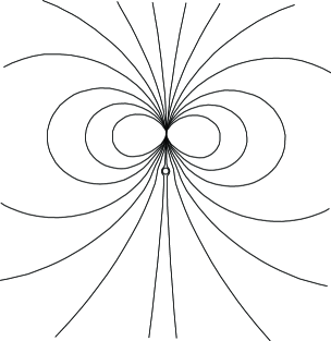
In our extensive paper [8] we developed the formalisms for the interacting perturbations of the Reissner-Nordström black holes in detail and clarified the relations between them. First we expanded Moncrief’s theory: all Hamilton equations following from four Moncrief’s Hamiltonians (for , and in both parities) are derived in suitable forms and from them the wave equations for gauge invariant perturbations are obtained. Starting then from the Hamilton equations and employing the relations between the standard form of perturbations, and , and canonical variables, one can express all ’s and ’s in terms of gauge invariant variables (satisfying the wave equations) in a suitable gauge. In [8] this is done in Regge-Wheeler gauge for perturbations and in another suitable gauge for the dipole perturbations. These results enabled us to treat various perturbation problems (as, for example, the expulsion of the field lines illustrated in Figure 1) and also to establish a detailed relation between the standard (Zerilli-type) perturbation formalism and the canonical (Moncrief-type) treatment of perturbations.
Of course, the coupled perturbations of the Reissner-Nordström black holes were analyzed also in the framework of the Newman-Penrose formalism which proved to be so efficient in the case of rotating black holes. Lun, Chitre, Lee and Chandrasekhar (see [7], [8] or [9] for references) are among the main contributors to the theory. Their results are extended in [8] in the following points: (i) the fundamental perturbation variables which satisfy decoupled equations are not only coordinate gauge invariant but also invariant under infinitesimal transformations of the Newman-Penrose tetrads; (ii) the dipole perturbations are analyzed in the Newman-Penrose formalism for the first time, and they are treated simultaneously with the perturbations; (iii) the relations between the canonical and the Newman-Penrose basic quantities are established.
We are recalling these results not only because they form the theoretical framework for solving the problems like the motion of a charged black hole in an asymptotically uniform electric field [10], or the fields of stationary sources on the Reissner-Nordström background [6]. A somewhat ‘central-European’ character of the journal in which [8] appeared, brings its “fruits”: in 1995 the formalism for the dipole odd-parity perturbations of the Reissner-Nordström solution was redeveloped in [11] and in 1999 the even parity case was treated [12] without a realization that this was done in [8] within the framework of three different formalisms. We believe that in [8] the most complete discussion is given of the interconnections between the standard, the canonical and the Newman-Penrose formalisms even for perturbations of Schwarzschild black holes.
Now there exist simple exact stationary multipole solutions for coupled perturbations of the Reissner-Nordström black holes [13]. (Some of these solutions have very recently been employed to study the electromagnetic Thirring effects [14].) In [6] we used these solutions to construct the magnetic field of a current loop (magnetic dipole) placed axisymmetrically on the polar axis of the extreme Reissner-Nordström black hole. The electromagnetic and gravitational field occurring when the general Reissner-Nordström black hole is placed in an asymptotically uniform magnetic field was also derived.
The magnetic lines of force, as introduced by Christodoulou and Ruffini (see [15] and references therein), were constructed numerically for all the sources mentioned above at various positions. We refer to [6] for details. Here, as an illustration, we present Figure 1 (From [6]), showing magnetic lines of force of the small current loop (magnetic dipole) located axisymmetrically on the polar axis of the extreme Reissner-Nordström black hole. One can make sure that the structure of the closed lines of force in the region ‘opposite’ to the place where the magnetic dipole is located (Figure 1b), is caused by the coupling of electromagnetic and gravitational perturbations. Owing to the extreme character of the black hole, no line of force crosses the horizon.
3. The flux of stationary magnetic fields across rotating black holes
In order to investigate the structure of an asymptotically uniform test magnetic field on the background of a Kerr black hole we can start from the field given explicitly in [16]. Without repeating here complicated formulas, let us recall that each can be expressed as a sum of two terms, one being proportional to , the magnitude of the component of the field asymptotically aligned with the hole’s rotation axis, the other, , being the magnitude of the component perpendicular to the axis. Following Christodoulou and Ruffini [15] we define the magnetic (electric) lines of force as the lines tangent to the direction of the Lorentz force experienced by a test magnetic (electric) charge at rest with respect to the locally non-rotating frame. For the magnetic field lines this definition yields and .


(a) (b)
In the case of the aligned field we can easily verify (by using from [16]) that the field lines lie on the surfaces of constant flux,
| (4) |
where
| (5) |
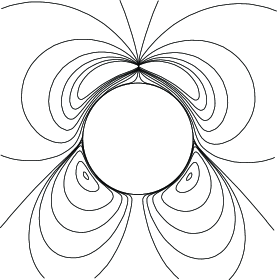
are Boyer-Lindquist coordinates. The field lines constructed numerically are shown in Figure 2. The figures clearly illustrate how the magnetic field is expelled from the horizon when the angular momentum of the hole increases. Analogously to the Reissner-Nordström case, no field line of the asymptotically uniform magnetic field enters the horizon of an extreme Kerr black hole.
In the case of general stationary axisymmetric (i.e. “aligned”) electromagnetic fields, one arives, using solutions given in [17] (in the Newman-Penrose formalism), at a similar result: the flux of an arbitrary, axially symmetric stationary magnetic field across any part of the horizon of an extreme Kerr black hole vanishes.
The structure of an asymptotically non-aligned field is much more complicated. In this case and the field lines are dragged around the black hole. The lines, originally parallel to each other, are twisted, some of them threading the horizon even in an extreme case. The results of the numerical construction of the magnetic lines asymptotically perpendicular to the rotation axis of the Kerr black hole with , as they look in the equatorial plane when viewed from above, are given in [18]. The field lines in Boyer-Lindquist coordinates are wound up around the horizon; in the Kerr ingoing coordinates the field lines do not wind up.
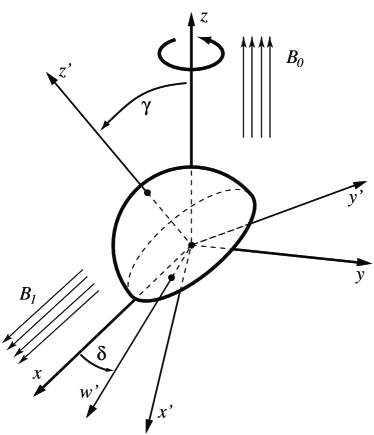
The structure of the magnetic field near a black hole can be characterized by the magnetic flux across (half of) the horizon. A general position of the hemisphere can be specified on the basis of an Euclidean picture. The magnetic flux across the hemisphere can be defined invariantly as an integral over the surface of the horizon [16]
| (6) |
where - see Figure 3.
Substituting for and performing the integral we find rather complicated expression which, however, can be understood intuitively in special cases: (i) If the magnetic flux reduces to ; with the total flux of the component of course vanishes. As the hole becomes extreme we find – see Figure 2 (c-d). (ii) If the flux is . If the hole is not rotating one gets . We get zero flux for and maximal one for . When the hole rotates the field lines are dragged along and the flux vanishes across the hemisphere rotated by an angle where for . For a given there exists for which the flux is maximal. With we find , . Hence, we see that although the flux of the aligned component decreases to zero with , the flux of the perpendicular component is enhanced.
4. Magnetic flux across the stretched horizon of an almost extreme Kerr black hole
In this section we shall outline some results of [19] and of the discussions one of us (J.B.) had with Richard Price in 1996. The discussions were concerned with the validity of the membrane paradigm [1] for ‘alex’ black holes, as we call ‘almost extreme’ black holes. It is well-known that a proper distance from any point outside an extreme black hole to the outer horizon is infinite. This fact implied the statement in [1], p. 120, that ‘because the horizon is infinitely far down in the [embedding] diagram, the finite magnetic flux has an infinite spatial distance in which to wrap itself around the embedding cylinder, and, consequently, near the horizon the magnetic field falls off to zero.’
Notice, first, that in fact in a freely falling frame the component and do not vanish at the horizon of an extreme Kerr black hole, only the radial component . (In case of an extreme Reissner-Nordström black hole all components of magnetic field do vanish even in a freely falling frame at the horizon.) Now in the spirit of the ‘membrane paradigm’ consider a flux across a stretched horizon characterized (in the Boyer-Lindquist coordinates) by the redshift factor for locally non-rotating frames (‘lapse function’),
| (7) |
which at a stretched horizon is small, , but nonvanishing - in contrast to the true horizon for which . Introduce a parameter so that is small for alex black holes and vanishes for the extreme holes. We know that the magnetic flux of axisymmetric fields vanishes at the true horizon in the limit :
| (8) |
A question arises whether if we ‘exchange’ the limits, i.e., calculate first the flux across the stretched horizon of an alex black hole and then go to the extreme case we could obtain a nonvanishing quantity: will then
| (9) |
Restricting ourselves to asymptotically uniform fields we can easily calculate the flux across the stretched horizon (using the expressions for electromagnetic field given in [16]) and find that
| (10) |
Therefore, across the stretched horizon is nonvanishing even in the extreme case but it depends on where is located; however, as , so that the limit (9) vanishes. For any there exists such that and . This conclusion seems to suggest that power in the Blandford-Znajek model arises from regions with ‘relatively large’ in near-extreme case.
5. Black holes in magnetic fields: exact models
We now turn to the exact stationary solutions of the Einstein-Maxwell equations representing rotating, charged black holes immersed in an axisymmetric magnetic field. In the weak-field limit – when , the constant in the weak-field limit characterizes the magnetic field strength, the hole’s mass – there exists a region where the spacetimes are approximately flat and the magnetic field is approximately uniform. At the metrics approach Melvin’s magnetic universe.
The simplest example is the magnetized Schwarzschild black hole:
| (11) |
where , the electromagnetic field being given by , . The magnetic flux across a general hemisphere on the horizon (with due to axisymmetry, cf. Figure 3) reads as follows:
| (12) |
For the flux across the ‘upper half’ of the horizon , we obtain the result given in [16]. (See Eq. (41) therein where incorrect should be replaced by in the denominator.)
If the flux is equal to in accordance with the weak-field approximation. By increasing (with and fixed) first increases, as we expect on classical grounds. However, a further increase of leads to the decrease of the flux. Indeed, there exists a value of the magnetic field parameter for which the flux acquires its maximum value, . The global maximum, occurring with , is
| (13) |
The existence of the limiting value of the magnetic flux across the horizon is caused by the gravitational effect of the magnetic field which concentrates itself near the axis of symmetry when .
In [4], a rather exotic but interesting model was presented recently in which a supermassive black hole is surrounded by a superstrong magnetic field of the strength corresponding to just the half of the maximal flux (13). In this model an electric induction field can accelerate charged particles up to an energy GeV.
There exists a fairly extensive literature on exact solutions representing rotating charged black holes in an external magnetic field (a magnetic Melvin-type universe). They can be used to study the Meissner effect within the exact framework. One can make sure that the magnetic fluxes vanish across the horizons of extreme black holes, i.e. those with zero surface gravity. We refer to [20] and to very recent paper [21] for the review and relevant references.
6. Meissner effect for superconducting branes and extremal black holes in string theory
In 1998 a comprehensive paper by Chamblin, Emparan and Gibbons [22] reviewed and developed evidence for the Meissner effect for extremal black hole solutions in string theory and Kaluza-Klein theory. Here we shall mention some of their ideas and results, sticking closely to their discussion. They first give a brief phenomenological description of the Meissner effect in superconductors. Using London equation
| (14) |
( - current, - vector potential), and Maxwell’s equations, one arrives at the equation
| (15) |
, given by constants characterizing the material. The solution in one dimension, , indicates that (and thus the magnetic field as well) decreases exponentially as one goes from the surface into the superconductive material. This is the classical Meissner effect. We see that the expulsion of a magnetic field from extreme (standard) black holes is analogous – but there is a difference: no magnetic flux at all penetrates into a hole. The relativistic generalization of the London equation reads
| (16) |
or
| (17) |
where is -current and 4-potential. In [22] equation (17) is adopted as the criterion for superconductivity. The authors first review the work of Nielsen and others showing that this equation is satisfied in the Kaluza-Klein theory on the world volume of extended objects carrying Kaluza-Klein currents. Then they consider self-gravitating extended superconducting objects and demonstrate how the flux of a gauge field is expelled from the intersection of two sets of 6-dimensional self-gravitating branes of 11-dimensional supergravity.
Several examples are then constructed in [22] demonstrating that the expulsion of gauge fields occurs always at the extreme horizon. Consider a string in which is wrapped along the string direction so that a dilatonic black hole solution in arises. The starting metric in reads
| (18) |
where , and are constants, an event horizon being at ; is the extreme case. If this geometry is compactified along the string direction in such a way that the compactification direction is twisted – the compactification is made along the orbits of the vector , where constant will describe the asymptotic value of the magnetic field along the axis – one obtains a black hole and the Kaluza-Klein magnetic field. The field is described by the potential whose - component is given by
| (19) |
In general one finds a non-vanishing flux across the horizon at . In the limit of an extreme hole, however, at the horizon the potential vanishes and no magnetic flux thus penetrates the horizon.
As another example of the Meissner effect Chamblin, Emparan and Gibbons consider the field expulsion from extreme rotating black holes. First they recall the expulsion of the asymptotic uniform magnetic test field in the extreme Kerr black hole background discussed in Section 3. Then they construct an exact solution (by taking the product of the standard Kerr solution with -direction and applying a twisted reduction procedure, similar to that considered above but involving also a twist in the time coordinate) representing a Kerr black hole in the exact Kaluza-Klein gauge field. Again, this exact field exhibits the Meissner effect in the extreme case.
At the end of the subsection (see [22], V. A.) the authors write that they considered the solutions in which the magnetic field is aligned with the rotation axis of the black hole but that according to our work [6] the Meissner expulsion can also be seen for fields where no alignment is assumed. This is not correct: as mentioned in the previous Section 3, and demonstrated in detail in [16], the asymptotically non-aligned fields do penetrate the extreme Kerr horizons. Only general axisymmetric, stationary fields on the Kerr background exhibit the Meissner effect in the extreme limit. On the other hand, it is well known that configurations with stationary external fields which are not axisymmetric, are not stable – due to the torque exerted on the horizon by an external non-axisymmetric field (see e.g. [1]) - and evolve towards axisymmetric configurations.
In case of the standard superconductivity, when the Meissner effect arises, the field inside a superconductor becomes a pure gauge. This is not the case with extreme black holes. In [6] in Figure 1(d) the field lines are constructed inside the extreme Reissner-Nordström horizon. Clearly, one cannot claim that the interior of extreme black holes is in a superconducting state.
The question of the flux expulsion from the horizons of extreme black holes in more general frameworks is not yet understood properly. The authors of [22] ‘believe this to be a generic phenomenon for black holes in theories with more complicated field content, although a precise specification of the dynamical situations where this effect is present seems to be out of reach.’ That for abelian Higgs vortices the phenomenon of flux expulsion from extreme black holes does not occur in all cases has been argued analytically and investigated numerically recently [23]. In particular, it appears that thin cosmic strings (modelled by the vortices) can pierce the extreme horizons whereas a thicker string will be expelled.
7. Black holes under the influence of external rings and disks: exact models
We shall now briefly pay an attention to the recent work of Semerák, Zellerin and Žáček [24], [25] in which exact solutions are constructed, representing static axisymmetric matter distributions around non-rotating black holes. There exists an extensive literature on disks surrounding black holes. The disks are usually treated as a test matter, or within a perturbation theory, or by numerical techniques. We refer to the Introduction in [24] for a number of citations to relevant papers.
In new work [24] Semerák et al used the ‘old’ fact that in case of static axisymmetric vacuum spacetimes Einstein’s equations reduce considerably: one equation becomes Laplace’s equation for one metric function, the other equation determines the second function in terms of a quadrature. The linearity of Laplace’s equation enables one to find fields representing ‘superposed sources’. In the standard Weyl coordinates the Schwarzschild black hole with mass is well known to be described by a rod of length (cf. [26]) along the axis of symmetry. In [24] this source, and also the Appell ring (the potential field generated by a particle situated on the imaginary extension of the axis of symmetry), is superposed with the following additional sources in the equatorial plane: (i) the Bach-Weyl ring (a ‘standard’ ring placed in the equatorial plane), (ii) the annular disk. The authors of [24] construct the complete fields and then plot nice figures illustrating the ‘gravitational field lines’ (defined as integral curves of the acceleration fields) in all three cases for various values of masses of the hole and the ‘external’ source. In another set of figures they illustrate the distortion of the Schwarzschild horizon caused by the presence of the external matter. In the second paper [25] a detailed description is given of how the motion of test particles is influenced by the superposed fields, in particular how the equatorial geodesics are modified when, for example, the mass of an external disk-like source is gradually increased.
8. The spinning C-metric: an exact model of accelerating, rotating black holes
The static part of a spacetime representing the standard, non-spinning vacuum C-metric was originally found by Levi-Civita in 1917-1919 (see references in [26]) but it was only in 1970 when Kinnersley and Walker understood, by choosing a better parametrization, that it can be extended so that it represents two black holes uniformly accelerated in opposite directions. The “cause” of the acceleration is given by nodal (conical) singularities (“strings” or “struts”) along the axis of symmetry. By adding an external gravitational field the nodal singularities can be removed [27]. If the holes are electrically (magnetically) charged the field causing the acceleration can be electric (magnetic) [28,10]. These types of generalized C-metric have been recently used in the context of quantum gravity - to describe production of black hole pairs in strong background fields (see e.g. [29]).
From the 1980’s several other works analyzed the standard C-metric. In none of these works, however, has the basic fact been emphasized that the vacuum C-metric is just one specific example in a large class of asymptotically flat radiative spacetimes with boost-rotation symmetry (with the boost along the axis of rotational symmetry). From a unified point of view, boost-rotation symmetric spacetimes with hypersurface orthogonal axial and boost Killing vectors were studied geometrically in [30]. We refer to this detailed work for rigorous definitions and theorems. In fact it is no surprise that the C-metric was for a long time analyzed in coordinate systems unsuitable for treating global issues such as the properties of null infinity. It is algebraically special, and the coordinate systems were adapted to its degenerate character. In polar coordinates the metric of a general boost-rotation symmetric spacetime with hypersurface orthogonal axial and boost Killing vectors, and , has the form (see [30], Eq. (3.38)):
| (20) | |||||
| (21) | |||||
| (22) |
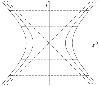
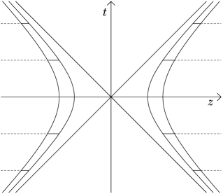
where and are functions of and , satisfying, as a consequence of Einstein’s vacuum equations, a simple system of three equations, one of them being the wave equation for the function . The whole structure of the group orbits in boost-rotation symmetric curved spacetimes outside the sources (or singularities) is the same as the structure of the orbits generated by the axial and boost Killing vectors in Minkowski space. In particular, the boost Killing vector is timelike in the region . It is this region which can be transformed to the static Weyl form. Physically this corresponds to the transformation to “uniformly accelerated frames” in which sources are at rest and the fields are time independent.
However, in the other “half” of the spacetime, (“above the roof” in the terminology of [30]), the boost Killing vector is spacelike so that in this region the metric (22) is nonstationary. It can be shown that for the metric can be locally transformed into the metric of the Einstein-Rosen waves. The radiative properties of the specific boost-rotation symmetric spacetime were investigated in a numer of papers; these spacetimes were also used as test beds in numerical relativity - see the review [31] for more details and references.
Now in all the work mentioned above it was assumed that the axial and boost Killing vectors are hypersurface orthogonal. Recently, we analyzed symmetries compatible with asymptotic flatness and admitting gravitational and electromagnetic radiation [32]. We have shown that in axially symmetric electrovacuum spacetimes in which at least locally a smooth null infinity exists, the only second allowable symmetry which admits radiation is the boost symmetry. The axial and an additional Killing vector have not been assumed to be hypersurface orthogonal. In [32] the general functional forms of gravitational and electromagnetic news functions, and of the total mass of asymptotically flat boost-rotation symmetric spacetimes at null infinity have been obtained. However, until now no general theory similar to that given in [30] in the hypersurface orthogonal case is available for the boost-rotation symmetric spacetimes with Killing vectors which are not hypersurface orthogonal. Nevertheless there is one explicitly given metric which can be expected to serve as an example of these spacetimes - the spinning vacuum C-metric. It was discovered by Plebański and Demiański [33] in 1976. However, its boost-rotation character has not been analyzed. In particular, “the canonical coordinates” in which the metric represents a generalization of the metric (22) so that global issues outside the sources could properly be studied have not been found so far.
In our recent work [34] we found such a representation of the spinning C-metric (SC-metric) which generalizes (22) and, thus, can also serve as a convenient example for building up the general theory of boost-rotation symmetric spacetimes with the Killing vectors which are in general not hypersurface orthogonal.
We first specialized the Plebański-Demiański class of metrics [33] to the spinning vacuum case, discussed the ranges of parameters entering the metric and indicated the limiting procedure leading to the Kerr metric. Then the SC-metric was transformed into Weyl coordinates. We showed that, by choosing different values of the original Plebański-Demiański coordinates we can, in principle, arrive at various Weyl spacetimes. The properties of Killing vectors and of some invariants of the Riemann tensor led us to choose a physically plausible Weyl spacetime which contains both the black-hole and the acceleration horizon. Similarly as has been done with the standard C-metric [35], we concentrated on this Weyl portion. Remarkably, the metric can then be also transformed into the “canonical form” of boost-rotation symmetric spacetimes:
| (23) | |||
| (24) |
where , and are functions of and , connected with the original Plebański-Demiański coordinates and with the Weyl coordinates in a quite complicated manner (see [34] for details).
The form (24) represents a general boost-rotation symmetric spacetime “with rotation”, i.e., with the Killing vectors which are not hypersurface orthogonal. Putting , we recover the canonical form of the boost-rotation symmetric spacetimes with the hypersurface orthogonal Killing vectors the general structure of which was studied in [30] .
Analogous to the C-metric without spin, the axis of symmetry contains nodal singularities between the spinning “sources” (holes) which cause the acceleration, and is regular elsewhere; or the axis can be made regular between the sources but then the nodal singularities extend from each of the sources to infinity (see Fig. 4 taken from [34]).
Acknowledgments.
I am very grateful to the organizers of ICGC 2000 for their hospitality. I thank Tomáš Ledvinka for constructing the figures and help with the manuscript. Support from the grant No. GAČR 202/99/0261 of the Czech Republic and the Grant J13/98:113200004 is also gratefully acknowledged.
REFERENCES
- [1] Thorne, K. S., Price, R. H. and MacDonald, D. A., Black Holes: The Membrane Paradigm, (Yale University Press, New Haven) 1986.
- [2] Burko, L., Ori, A., Introduction to the internal structure of black holes, in Internal Structure of Black Holes and Spacetime Singularities, eds. L. Burko and A. Ori, (Inst. Phys. Publ., Bristol and The Israel Physical Society, Jerusalem) 1997.
- [3] Mirabel, I. F., Rodríguez, L. F., Microquasars in our Galaxy, Nature, 392 (1998) 673.
- [4] Kardashev, N. S., Cosmic supercollider, Mon. Not. R. Astron. Soc., 276 (1995) 515.
- [5] Frolov, V., Novikov, I., Physics of Black Holes, (Kluwer, Dordrecht) 1998.
- [6] Bičák, J., Dvořák, L., Stationary electromagnetic fields around black holes III. General solutions and the fields of current loops near the Reissner-Nordström black hole, Phys. Rev. D, 22 (1980) 2933.
- [7] Chandrasekhar, S., The Mathematical Theory of Black Holes, (Clarendon Press, Oxford) 1984.
- [8] Bičák, J., On the theories of the interacting perturbations of the Reissner-Nordström black hole, Czechosl. J. Phys., B29 (1979) 945.
- [9] Bičák, J., Perturbations of the Reissner-Nordtröm black hole, in Proceedings of the 2nd M. Grossmann Meeting on General Relativity, ed. R. Ruffini, (North Holland) 1982, p. 277.
- [10] Bičák, J., The motion of a charged black hole in an electromagnetic field, Proc. Roy. Soc. Lond., A371 (1980) 429.
- [11] Burko, L. M., Dipole perturbations of the Reissner-Nordström solution: The Polar Case, Phys. Rev. D, 52 (1995) 4518.
- [12] Burko, L. M., Dipole perturbations of the Reissner-Nordström solution: The axial case Phys. Rev. D, 59 (1999) 084003.
- [13] Bičák, J., Stationary interacting fields around an extreme Reissner-Nordström black hole, Phys. Lett., 64A (1977) 279.
- [14] King, M., Pfister, H., On Electromagnetic Thirring Problems, to be submitted to Phys. Rev. D.
- [15] Christodoulou, D., Ruffini, R., On the Electrodynamics of Collapsed Objects, in Black Holes, eds. C.DeWitt and B. deWitt (Gordon and Breach, London) 1973.
- [16] Bičák, J., Janiš, V., Magnetic fluxes across black holes, Mon. Not. Roy. Astron. Soc., 212 (1985) 899.
- [17] Bičák, J., Dvořák, L., Stationary electromagnetic fields around black holes II. General solutions and the fields of some special sources near a Kerr black hole, Gen. Rel. Grav., 7 (1976) 959.
- [18] Karas, V., Asymptotically uniform magnetic field near a Kerr black hole, Phys. Rev. D, 40 (1989) 2121.
- [19] Price, R. H., Some Developments in Black Hole Astrophysics, Ann. N.Y. Acad. Sci., 631 (1991) 235.
- [20] Bičák, J., Karas, V., The influence of black holes on uniform magnetic fields, in Proc. of 5th M. Grossmann Meeting in General Relativity, eds. D. Blair et al (World Scientific, Singapore) 1989, p. 1199.
- [21] Karas, V., Budínová, Z., Magnetic Fluxes Across Black Holes in a Strong Magnetic Field Regime, Physica Scripta, 61 (2000) 253.
- [22] Chamblin, A., Emparan, R. and Gibbons, G. W., Superconducting p-branes and extremal black holes, Phys. Rev. D, 58 (1998) 084009.
- [23] Bonjour, F., Emparan, R. and Gregory, R., Vortices and extreme black holes: the question of flux expulsion, Phys. Rev. D, 59 (1999) 084022.
- [24] Semerák, O., Zellerin, T. and Žáček, M., The structure of superposed Weyl fields, Mon. Not. Roy. Astron. Soc., 308 (1999) 691.
- [25] Semerák, O., Zellerin, T. and Žáček, M., The test-particle motion in superposed Weyl fields, Mon. Not. Roy. Astron. Soc., 308 (1999) 705.
- [26] D. Kramer, H. Stephani, M. MacCallum and E. Herlt, Exact solutions of Einstein’s Field Equations, (Cambridge University Press) 1980.
- [27] F. J. Ernst, Generalized C-metric, J. Math. Phys., 19 (1978) 1986; W. B. Bonnor, An exact solution of Einstein’s equations for two particles falling freely in an external gravitational field, Gen. Rel. Grav., 20 (1988) 607.
- [28] F. J. Ernst, Removal of the nodal singularity of the C-metric,J. Math. Phys., 17 (1976) 515.
- [29] S. W. Hawking, G. T. Horowitz and S. F. Ross, Entropy, area, and black hole pairs,Phys. Rev. D, 51 (1995) 4302.
- [30] J. Bičák, B. G. Schmidt, Asymptotically flat radiative space-times with boost-rotation symmetry: The general structure, Phys. Rev. D, 40 (1989) 1827.
- [31] J. Bičák, Radiative spacetimes: exact approaches, in Relativistic Gravitation and Gravitational Radiation, Proceedings of the Les Houches School of Physics, edited by J. A. Marc and J. P. Lasota, (Cambridge University Press, Cambridge) 1995.
- [32] J. Bičák, A. Pravdová, Symmetries of asymptotically flat electrovacuum spacetimes and radiation, J. Math. Phys., 39 (1998) 6011.
- [33] J. F. Plebański, M. Demiański, Rotating, charged and uniformly accelerating mass in general relativity, Annals of Phys., 98 (1976) 98.
- [34] Bičák, J., Pravda, V. Spinning C-metric: radiative spacetime with accelerating, rotating black holes, Phys. Rev. D, 60 (1999) 044004.
- [35] W. B. Bonnor, The sources of the vacuum C-metric, Gen. Rel. Grav., 15 (1983) 535.